PHYSOR 2004 -The Physics of Fuel Cycles and Advanced Nuclear Systems: Global Developments Chicago, Illinois, April 25-29, 2004, on CD-ROM, American Nuclear Society, Lagrange Park, IL. (2004)
Variance Reduction Techniques for the Monte Carlo Simulation of Neutron
Noise Measurements
Máté Szieberth*1 and Jan Leen Kloosterman2
1 Budapest University of Technology and Economics, 1111 Budapest, Műegyetem rkp. 9., Hungary 2 Delft University of Technology,2629 JB Delft, Mekelweg 15, The Netherlands
This paper presents the theory and methods to apply variance reduction techniques in the Monte-Carlo simulation of neutron noise experiments. Conventional Monte-Carlo variance reduction techniques are not applicable, because the behavior of the neutron noise depends on the collective effects of particles, and furthermore is influenced by the higher-moments of the tally distribution, which are not preserved by these methods.
The application of variance reduction methods results in weighted counts and undesired correlations from the splitted particles. A theory is developed and a correction is derived for the bias caused by the introduction of particle weights. The history splitting method is proposed to destroy the undesired correlations caused by particle splitting. The new method makes possible the application of a variety of variance reduction techniques, except for Russian roulette, which must be replaced by alternative history control methods.
The described techniques were implemented in MCNP4C and the results of preliminary calculations and comparison with analogue calculations are shown to prove the feasibility of the proposed method.
KEYWORDS: Monte Carlo, variance reduction, neutron noise analysis, Feynman-α method, variance-to-mean ratio
*
Corresponding author, Tel. +36-1-4631633, FAX +36-1-4631954, E-mail: [email protected]
1. Introduction
At present accelerator driven systems (ADS) are being studied, because of the attractive features with regard to safety and transmutation. A crucial point for the practical realization of ADS is the development of a reliable method to monitor the reactivity of the core. Among others, neutron noise methods such as Feynman-α and Rossi-α measurements are being proposed for this, and experiments like the MUSE project are being conducted to investigate how these techniques can be applied to ADS. Furthermore, new theories are being developed to describe these methods in a more sophisticated way with special attention to spatial, spectral and temporal effects. The development of computer codes that can assist in the design and analysis of neutron noise experiments systems has outstanding importance.
Conventional Monte-Carlo codes applying variance reduction techniques are not applicable, because the behavior of the neutron noise depends on the collective effects of particles, which can be only estimated by so-called non-Boltzmann tallies [1], and furthermore is influenced by the higher-moments of the tally distribution, which are not preserved by these codes. Therefore, modified versions of existing well-known Monte Carlo codes have appeared like KENO-NR [2], MCNP-DSP [3] and MVP [4]. In these codes, the real distribution of fission neutrons is sampled as well as the direction of fission neutrons relative to the incident neutron [5].
Furthermore, the simulation of detection events is done in a fully analogue way: one count is generated for each detector event (capture, fission, scattering, etc.). The counts detected during a predefined period (block) are collected into time bins and processed by the built-in digital signal processing (DSP) routines. The output of this calculation is the result of the simulated experiment. As a result of the analogue algorithm, the above-mentioned codes need long CPU times to arrive at acceptable statistics. This causes serious problems if one has to model a large and complicated geometry or if the detector efficiency is very low, which is usually the case in fast reactors.
This paper presents the theory and the methods to apply variance reduction techniques in the Monte-Carlo simulation of neutron noise experiments in a way that circumvents the above problems.
2. Theory and methods to apply variance reduction methods 2.1 Introduction of the particle weight
The weight of a particle, which is proportional to the probability of the given particle track, is a basic principle for Monte Carlo variance reduction techniques. With the introduction of weight the analogue simulation of detection events is not feasible anymore: instead of having a few integer counts, one gets many fractional detector contributions. The expected value of the sum of all weighted counts (W) equals the expected value of the number of counts (N) as the introduction of the weight preserves the mean value, but reduces considerably the variance.
1 t N i i N w = =
∑
= W (1)As noise analysis techniques are usually governed by the higher moments, corrections are needed. In the following paragraphs the required corrections for the Feynman-α and the autocorrelation method are derived.
2.1.1 Feynman variance-to-mean method
The Feynman-α method needs special attention, because it uses the variance of the measured data. The variance to mean ratio is described by [6]:
( )
2 2 1 1 1 1 1 1 1 T T p N D e e Y N T T α α ν σ ε ρ α α − − ∞ ⎛ − ⎞ ⎛ − ⎞ = + ⎜ − ⎟= + ⎜ − ⎟= + ⎝ ⎠ ⎝ ⎠ Y (2)where Dν is the Diven-factor, ρp is the prompt reactivity and α is the prompt neutron decay
constant. Y usually denotes the correlated part, which measures the deviation from the Poisson distribution, while Y∞is its asymptotic value. Let λ be the expected value of the number of
counts in a detector with volume V and reaction cross-section during a time interval T:
( ) (
)
0 0 , , T V E E t dEdVdt λ=∫∫∫
∞Σ Φ r (3)As it was shown in an earlier paper [7] the correlated part of the variance to mean ratio equals to the variance to mean ratio of λ, which is related to the stochastic nature of the neutron transport.
( )
( )
2 2 1 = N N σ σ λ λ + (4)It was shown as well, that the introduction of the weighted counts to the detection effects the uncorrelated part only.
( )
( )
2 W 2 2 m W m σ σ λ σ λ = + + (5)From (4) and (5) the following correction formula can be obtained for the introduced negative offset[7]:
( )
( )
2 2 2 1 N W m N W m σ −σ = −σ − , (6)where m is the mean value while σ2 is the variance of the weight of a single count. Usually, these two parameters can be estimated very accurately, because there are many more fractional counts than real counts. Assuming real counts with a weight of one, the variance of the weights becomes σ2=0, while the mean is m=1, and (6) becomes zero.
2.1.2 Autocorrelation function
The autocorrelation can be written as:
2 2 1 2 1 2 1 0 ) ( N N N N N N N ACF τ = τ = τ (7)
where N1 means the number of counts in a time interval [t,t+∆t] and N2 means the number of
counts in a time interval [t+τ,t+τ+∆t]. As the denominator equals the second moment, which is not preserved, a correction is needed[7]:
(
)
2 2 2 2 W N W W m m σ = + − + (8)The obtained formula can be calculated as simple as (6). Furthermore holds that the correction becomes zero in the case of real counts.
2.2 Particle splitting methods 2.2.1 History splitting
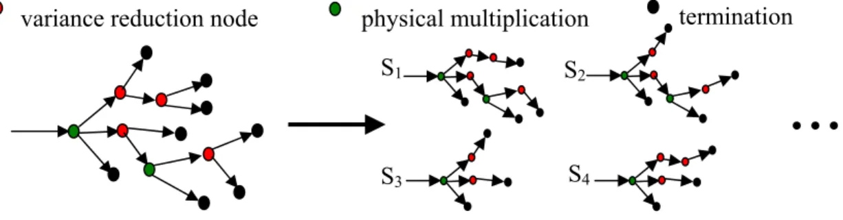
To cope with the problem of detectors located far away, variance reduction techniques like particle splitting are used in Monte Carlo transport calculations. The basic idea is to increase the neutron population in the region of interest (close to the detectors) by splitting the particle and to reduce the weight of each particle such that the sum of all weights is preserved [8]. Unfortunately, this method cannot be applied to the simulation of neutron noise experiments, because of the extra correlation between the particles originating from the splitting process. With the application of the history splitting method proposed, this undesired correlation can be avoided. This method explained in the following paragraphs is very similar to the so-called deconvolution approach developed by Booth [1] for non-Boltzmann tallies and especially for pulse height tallies.
S3 S4
S2 S1
termination physical multiplication
variance reduction node
...
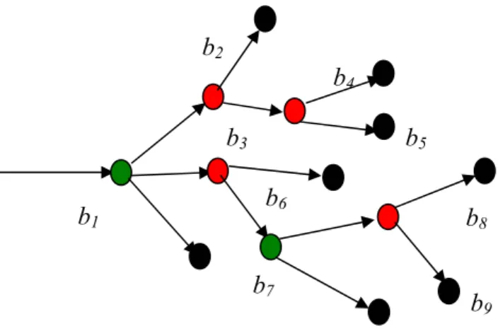
b9 b8 b5 b6 b7 b4 b3 b2 b1
Figure 2 The physical branches (bi) in a history
History splitting implies that upon a particle splitting the whole history is split and each originating particle is assigned to a separate history. In this way one source event generates multiple histories with reduced weight. Then these histories are subsequently treated as independent ones with different source times to avoid the extra correlation between the particles but to preserve the real correlation.
Figure 1 shows a simple Monte Carlo neutron history tree to demonstrate the basic principals of the method. In the original history on the left-hand side the physical multiplications (fissions) in the history are indicated with green dots, while the red ones are the variance reduction nodes. Tracks bordered by these nodes are the physical branches (see Fig. 2). The original history should be split in such a way that in the new sub-histories (examples on the RHS of Fig. 1) only one possible branch (track) is followed at every variance reduction node because these subhistories are supposed to represent real physical neutron chains. While in the Monte Carlo transport history the weight of the tracks changes at every splitting, one single weight is assigned to each subhistory from the source to the termination. The sum of the weights of the subhistories gives the weight of the original source particle. After the termination of each history the subhistories should be generated. To do this, data should be recorded from each variance reduction node during the conventional Monte Carlo transport calculation. These data are the parent-branch, the daughter-branches and their weights. The weight of a branch is defined as the weight reduction suffered by the track at the given node. This way the weight (Wi) of a given subhistory (Si) is the product of the weights (wi) of all its
branches (bi):
i j j
j
W =
∏
w b ∈Si (9)The number of the subhistories can be easily determined in a recursive way: the possibilities from one node can be calculated by summing up the possibilities from its daughter-branches while the possibilities from a branch are obtained from the product of the possibilities from its daughter-nodes. This warns for the careful use of variance reduction because the number of generated subhistories increases geometrically. The above described method was realized for several variance reduction methods.
2.2.2 Replacement of Russian roulette
Russian roulette (RR) is a basic method to control the spread and the weights in a history. Under certain conditions (e.g.: weight below cutoff) a track is removed (w=0) with a probability of p or it survives with an increased weight (w'=w/p)[8]. In the case of the above described approach the RR game is played on every subhistory to which the given branch belongs. This means that several Russian roulette games can be played on a subhistory and each of them can
kill it. This results in a very low survival probability (pn, where n is the number of Russian roulette games) and high survival weight. The resulting badly sampled high importance contributions can destroy the advantages gained from the application of variance reduction. Because of this problem the Russian roulette was avoided and other methods were used to control the histories. After certain limits were reached (e.g.: number of subhistories) the variance reduction techniques are switched off, and the history will soon terminate due to absorption. This method is far not so effective as the RR but much better suited to the history splitting method.
2.2.3 Implicit capture
In the case of the implicit capture at every collision the particle is split into an absorbed (w=σa/σt) and an unabsorbed (w=1-σa/σt) part[8]. Only the unabsorbed track is followed further. As the weight decreases continuously normally weight cutoff with Russian roulette is needed. When weigth drops below the cutoff, implicit capture is switched off. In order to control the number of subhistories the same happens when the number of implicit captures exceeds a certain limit.
2.2.4 Geometrical splitting
Geometrical splitting means that a particle is split into n pieces when it enters a region with n times higher importance[8]. The weight is set to w’=w/n. In the reverse direction RR should be played with probability 1/n but this was turned off. To prevent successive particle splittings on the same surface geometrical splitting is made only when the particle enters a region for the first time. Again this reduces the effectiveness of the method but circumvents the problems caused by RR.
2.2.5 Detection
The most important part of the simulation is the detection. The aim is to split every particle entering the detector into a detected and an undetected part which is done by the mechanism of implicit capture along the flight path[9]. When the particle travels through the detector, the distance to the next scattering (di at energy Ei) is sampled instead of the distance to the next
collision. In this manner the absorption is ruled out and is implicitly included along the whole flight path. Assuming that the detection cross-section (Σd) is part of the absorption one (Σa), the
particle can be split into an absorbed, a detected and an undetected part in the following way:
( )
( )
( )
(
( ))
( ) 1 1 1 1 a i i a j j N i E d E d a i d i abs i a i j E E w e E − −Σ −Σ = = Σ − Σ = − Σ∑
∏
e (10)( )
( )
(
( ))
( ) 1 1 1 1 a i i a j j N i E d E d d i det i a i j E w e E − −Σ −Σ = = Σ = − Σ∑
∏
e (11) ( ) 1 a i i N E d undet i w e−Σ = =∏
(12)where N is the number of straight flight paths in the detector. For the control of the number of originating subhistories this game is played on a track only when it passes through the detector for the first time. If the undetected part returns to the detector it is treated analogously.
2.2.6 Effect of the weighted source events
Although the history splitting method destroys the undesired correlations (which is enough to preserve the prompt decay constant of the system) it introduces an other bias by reducing the
variance of the source events. In the analogue case there are only source events with weight 1, which have a Poisson distribution in a given time interval. As the expected number of counts (λ, see (3)) can be interpreted as a sum of the contributions from the histories it is obvious that the distribution of the source events influences the higher moments of λ. This results in a bias in the correlated part of (5). Unfortunately, a correction cannot so easily be derived as for the uncorrelated part, because the weight of a subhistory is correlated with the number of detector contributions in it. (The more detector contribution a subhistory has; the lower is its weight because of more variance reduction games suffered.) This is why this bias is not corrected in the following preliminary calculations. Further analyses of the problem are in hand.
3. Preliminary calculations
3.1 Implementation in MCNP4C and calculations
The above described methods were implemented in MCNP4C[10]. Subroutines were added to collect the required data from variance reduction nodes (CREATENODE, CREATEBRANCH), and a function calculates the number of subhistories (GETSUBTREES). A special subroutine (SUBHISTORY) is called when a history is finished. It generates the subhistories by calling recursive subroutines (MAPNODE, MAPBRANCH) and writes into a file the weight of each subhistory, the detector contributions occurred in it together with their travelling time from the source to the detector. This file is processed by another code, which samples a source time for each subhistory, sorts by time and writes the time and weight of the counts into a “measurement” file. These data can then be analyzed by any kind of noise analysis technique similarly to a measured data file except for the required corrections because of the weighted counts (see (6) and (8))[7].
Furthermore, the required modifications to the physical model of neutrons were transferred from MCNP-DSP to MCNP4C without interfering with the original calculation flow. These modifications include the usage of the actual fission neutron distribution and the sampling of the direction of the fission neutrons relative to the incident neutron[3,5]. A new source option was created for spontaneous fission where multiple neutrons start at the same source position[7].
The above calculational system was applied for two simple problems: a thermal and a fast one (see Fig. 3a-b). The very simple geometry has been chosen so that even the analogous method can produce results with good statistics in a reasonable time.
3.1 Fast system
The examined problem was a Pu sphere 6 cm in radius (see Fig. 3a). The sphere was deeply sub-critical (keff=0.91030±0.00079) and the system was driven by spontaneous fission neutrons from 240Pu and 242Pu. Two lithium glass (5.08 cm in diameter, 2.54 cm long) detectors are located adjacent to the sphere and are positioned 180º apart.
Because of the vacuum around the detectors geometry splitting made no sense. Implicit capture (max. 3 times subsequently on a track) and implicit capture along the flight path for the detection was used. The simulation was switched to fully analogue mode when the number of subhistories in a history exceeded 5000.
a) b)
Figure 3a-b The MCNP model of the investigated fast (a) and thermal (b) system 3.2 Thermal system
The Pu sphere was placed in light-water and the radius was decreased to 5 cm to keep it subcritical (keff=0.95329±0.00118). The detectors were placed closer to the sphere to increase the efficiency.
This geometry was perfect to test the geometrical splitting method as the neutrons travel through the moderator. For this purpose three splitting surfaces were created around each detector (see Fig. 3b). The importance increases towards the detector 1.5 times on each surface, which results in a splitting to two with 50% probability. The implicit capture was switched off because it is not effective enough in this problem while the detection was made the same way as above. The cutoff in the number of subhistories was set to 1000 per history.
4. Results of the preliminary calculations
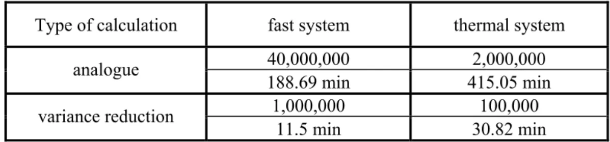
The results obtained from the above described preliminary calculations were analyzed with the Feynman variance-to-mean method. The basic data about the runs are summarized in Table 1. It can be observed that in the case of the fast system the save in CPU time is about a factor of twenty, while in the more time consuming thermal case it is about a factor of ten.
Table 1 Number of started histories and required CPU time for the calculations Type of calculation fast system thermal system
40,000,000 2,000,000 analogue 188.69 min 415.05 min 1,000,000 100,000 variance reduction 11.5 min 30.82 min
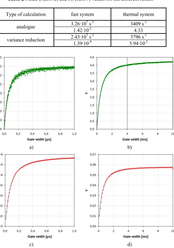
Some characteristic results and fitted curves are shown in Figure 4. The fitted parameters (see (2)) are shown in Table 2 as well. The figure shows that all results have good enough statistics for the comparison (in the variance reduction cases they are even slightly better despite the much shorter CPU time). The correction for the offset in the case of weighted counts (see (6)) was precise. The fitted alpha values are close in the analogue and variance reduction
cases, but the discrepancies are higher than expected: ~25% for the fast and ~10% for the thermal system, which is much higher than the standard deviation of the fitted parameters. The investigation of these discrepancies needs further work. As it was expected the history splitting method biases the asymptotic value (Y∞) in a high extent (see section 2.2.6).
Table 2 Fitted α (above) and Y∞ (below) values for the different results
Type of calculation fast system thermal system 3.26·107 s-1 3409 s-1 analogue 1.42·10-2 4.33 2.43·107 s-1 3796 s-1 variance reduction 1.39·10-9 5.94·10-2 0,0E+0 2,0E-3 4,0E-3 6,0E-3 8,0E-3 1,0E-2 1,2E-2 1,4E-2 1,6E-2 0,0 0,2 0,4 0,6 0,8 1, Gate width [µs] Y 0 a) 0,0 0,5 1,0 1,5 2,0 2,5 3,0 3,5 4,0 4,5 0 2 4 6 8 Gate width [ms] Y 10 b) 0,0E+0 2,0E-10 4,0E-10 6,0E-10 8,0E-10 1,0E-9 1,2E-9 1,4E-9 0,0 0,2 0,4 0,6 0,8 1,0 Gate width [µs] Y c) 0,00 0,01 0,02 0,03 0,04 0,05 0,06 0,07 0 2 4 6 8 Gate width [ms] Y 10 d)
Figure 4a-d Results for the fast (left) and the thermal (right) system with analogue (top) method and with variance reduction (bottom)
4. Conclusions
To speed up the simulation of neutron noise experiments, theory and methods were developed to make possible the application of variance reduction methods. It was shown that the introduction of the particle weight influences the uncorrelated part only, which can be corrected.
The application of particle splitting is possible with the help of the history splitting technique. The proposed method destroys the undesired correlations and preserves the prompt neutron decay constant of the system. However, the weighting of the source events introduces a bias to the asymptotic value of the correlated part. Correction for this distortion has not been developed yet. A variety of Monte Carlo variance reduction techniques were realized with the history splitting method. As the Russian roulette game was proved to be incompatible with this approach, it was replaced with alternative history control methods.
The history splitting method was implemented in MCNP4C and preliminary calculations were carried out for simple systems to prove its feasibility and to compare it with analogue calculations. The results show that the new method speeds up the calculations to a high extent. However it needs further development and investigations because some discrepancies were found compared to the analogue results.
Acknowledgements
The authors acknowledge the European Commission for co-funding this work under project number FIKW-CT2000-00063, and the other members of the MUSE project for their cooperation.
References
1) T. E. Booth, “Monte Carlo Variance Reduction Approaches for Non-Boltzman Tallies”,
LA-12433, Los Alamos National Laboratory (1992).
2) E. P. Ficaro, KENO-NR: “A Monte Carlo Code Simulating the 252Cf-Source-Driven Noise Analysis Experimental Method for Determining Subcriticality”, Ph.D. Dissertation,
University of Michigan (1991).
3) T. E. Valentine, “MCNP-DSP Users Manual”, ORNL/TM-13334, Oak Ridge National Laboratory (1997).
4) T. Mori, K. Okumura, Y. Nagaya, “Development of the MVP Monte Carlo Code at JAERI”,
Transactions of the ANS, 84, 45 (2001).
5) T. E. Valentine, “Review of subcritical source-driven noise analysis measurements”, ORNL/TM-1999/288, Oak Ridge National Laboratory (1999).
6) Robert E. Uhrig, “Random noise techniques in nuclear reactor systems”, The Roland Press
Company, New York (1970).
7) M. Szieberth, J. L. Kloosterman, “New methods for the Monte Carlo simulation of neutron
noise experiments”, Proc. Nuclear Mathematical and Computational Sciences, M&C2003, Gatlinburg, Tennessee, April 6-11, (2003).
8) I. Lux, L. Koblinger, “Monte Carlo Particle Transport Methods: Neutron and Photon
Calculations”, CRC Press, Boston (1991).
9) J.Spanier and E.M.Gelbard, “Monte Carlo Principles and Neutron Transport Problems”, Addison-Wesley, London (1969).
10)Briesmeister J.F. (ed.), “MCNP-A General Monte Carlo N-Particle Transport Code, Version