WP-2008-010
The Structure of Inflation, Information and Labour
Markets: Implications for monetary policy
Ashima Goyal
Indira Gandhi Institute of Development Research, Mumbai
May 2008
The Structure of Inflation, Information and Labour
Markets: Implications for monetary policy
1Ashima Goyal
Indira Gandhi Institute of Development Research (IGIDR) General Arun Kumar Vaidya Marg
Goregaon (E), Mumbai- 400065, INDIA Email (corresponding author): ashima@igidr.ac.in
Abstract
The paper gives a simplified version of a typical dynamic stochastic open economy general equilibrium models used to analyze optimal monetary policy. Then it outlines the chief modifications when dualism in labour and in consumption is introduced to adapt the model to a small open emerging market such as India. The implications of specific labour markets, and the structure of Indian inflation and its measurement are examined. Simulations give the welfare effects of different types of inflation targeting. Flexible CPI inflation targeting (CIT) without lags works best, especially if the economy is more open. But volatile terms of trade make the supply curve even steeper than in a small open economy despite specific labour markets and higher labour supply elasticity. Exchange rate intervention limits the volatility of the terms of trade and improves outcomes, making the supply curve flatter. As long as such intervention is required, domestic inflation targeting (DIT) continues to be more robust and effective. The welfare losses from the lags in CPI, which prevent the implementation of CIT, are low as long as the dualistic structure dominates. As the economy becomes more open, however, the loss from not being able to use CIT rises. The lags in CPI therefore need to be reduced, making its future use possible.
Key words: small open emerging market, optimal monetary policy, dualistic labour markets, inflation, measurement lags, specific labour markets
JEL Codes: E52, F41
1 The paper uses the model developed in Goyal (2007) to address new questions. The earlier paper was presented at IGIDR-RBI-Northwestern, ISI and IEG conferences in 2007. This paper was presented at the V.K.R.V Rao Centenary Conference on “National Income and other Macroeconomic Aggregates in a Growing Economy” April 28-30, Institute of Economic Growth and Delhi School of Economics, New Delhi. I thank Errol D’Souza, Gopal Kadekodi, Sabyasachi Kar, Hrushikesk Mallick, Rupayan Pal, and V.N. Pandit for helpful comments. and T. S. Ananthi, Jayashree and Reshma Aguiar for secretarial assistance.
The Structure of Inflation, Information and Labour
Markets: Implications for monetary policy
Ashima Goyal
1. Introduction
Consumer price indices in India are available only at monthly frequencies, with a two- month lag. Moreover, food items and services with administrative price interventions have a large weight in these indices. Consumer price indices are also not measured on an all India basis. Therefore there are both information and price adjustment lags in the CPI. So the wholesale price index (WPI), or domestic prices, is used as the
preferred measure for policy purposes. Worldwide CPI is used to target inflation since this is the measure that directly affects consumer utility and wage expectations.
Moreover, in an open economy there is the shortest lag from the exchange rate to consumer prices (Svensson 2000), making this an effective channel for monetary policy.
In this paper we adapt dynamic stochastic open economy general equilibrium models used to analyze optimal monetary policy2 to the labour market structure of a small open emerging economy. It is then possible to assess the welfare loss, if any, from domestic rather than consumer inflation targeting.
Since the policy response to shocks is analyzed using aggregate demand and supply curves derived from microfoundations, it is immune to the Lucas critique. The
coefficients of the model are based on deep parameters of preferences and technology that do not shift with the policy regime. But it has been necessary to put in various types of market imperfections in these types of models for them to be able to reproduce actual macroeconomic outcomes. The labour market is most critical for these outcomes. To hope to be able to reproduce the experience of a small open emerging market economy (SOEME), it is necessary to put in features of its labour market. We allow for a dualistic labour market with large numbers at subsistence employment. Equilibrium models allow unemployment to be driven only by an optimizing labour supply decision—which cannot capture the dimensions of
unemployment in a developing economy. The modeling of two types of labour makes it possible to capture this major aspect. Low productivity employment is the major coping mechanism in a SOEME for less than full employment in the productive modern sector. Our model has the usual product diversity and monopolistic
competition so that output is at less than the social optimal for this reason as well as for the low labour absorption in productive sectors. Sticky prices allow real effects of monetary shocks.
Labour markets are more segmented in a SOEME because of large skill differences so that the assumption of specific labour markets is better suited to them than economy-wide labour markets. In specific labour markets one labour type works to produce
2 Notable contributions in this area include Clarida, Gali and Gertler (1999, 2001), Obstfeld and Rogoff (1996), Svensson (2000) and Woodford (2003). Gali and Monacelli (2005) offer a detailed and rigorous application to a small open economy.
goods different from those the second type work in. In economy-wide markets a weighted average unit of labour is defined. In these circumstances it pays a firm to raise its prices if others are raising their prices—prices become strategic
complements. The output impact of a monetary shock rises—that is the aggregate supply curve becomes flatter.
We compare the welfare consequences of optimizing policy responses to shocks. The exchange rate is not itself a target variable but affects both output and inflation. In earlier results (Goyal 2007), when realistic lags were built into the CPI and flexible domestic inflation targeting (DIT) turned out to have the least welfare loss. Here we show flexible CPI inflation targeting (CIT) without lags works best, especially if the economy is more open. But exchange rate intervention that limits the volatility of the terms of trade improves outcomes. Terms of trade are volatile in a SOEME and this volatility makes the supply curve even steeper than in a small open economy (SOE) despite specific labour markets and higher labour supply elasticity. As long as
exchange rate intervention is required, DIT continues to be more robust and effective. The welfare losses from the lags in CPI, which prevent the implementation of CIT, are therefore minimal as long as the dualistic structure dominates. As the economy becomes more open, however, the loss from not being able to use CIT rises. Therefore the lags in CPI need to be reduced, making its future use possible.
Section 2 gives a highly simplified version of a typical SOE model. Section 3 outlines the chief modifications when dualism in labour and consumption is introduced. Section 4 analyzes the implications of specific labour markets, section 5 examines the structure of Indian inflation and its measurement, section 6 reports the calibrations and simulations, and section 7 concludes. Some derivations are in the appendix.
2. Basic SOE model
A microfoundation based SOE model is used to derive optimal monetary policy3. The key features are intertemporal optimization and labour-leisure tradeoff by consumers, monopolistic competition and product diversity so that producers have pricing power, and output is below the social optimum. The Calvo model of staggered prices
generates the sticky prices required for monetary policy to have real effects on output. The optimization results in simple standard aggregate demand (AD) and supply curves (AS) with the difference that they include forward-looking variables. These can be used to derive the optimal policy response to shocks.
The generic form of the objective function the representative consumer maximizes is:
(
t t)
t tu C N E , 0 0∑
∝ = β (1)Consumption, C, increases and labour, N, decreases the discounted present value of utility with β is the discount factor. Underlying the macro variables is CES aggregation, over i ∈ [0, 1] countries, and j ∈ [0,1] product varieties. Aggregate consumption, C, is derived from CES aggregation of consumption of home and foreign goods (
C
H,
C
F). If the elasticity of substitution between H and F goods is equal to unity, the CES aggregation collapses to Cobb-Douglas:
3 The model in this section is a simplified version of the Gali and Monacelli (2005, henceforth GM) small open economy model.
α α t F t H t kC C C = 1−, , (2) Where
(
−α)
−ααα = 1 1 1k is a constant and α is an index of openness. The associated
consumer price index (CPI) is:
( ) ( )
α α t F t H t P P P = , 1− , (3)CH, t is itself an index of consumption of domestic goods derived by CES aggregation with elasticity of substitution ε >1 over j domestic varieties. CF, t is an index of imported goods, derived by CES aggregation with elasticity of substitution γ =1 over imported goods j, from i countries of origin, Ci,t. Thus Ci,t is an index over j goods imported from country i and consumed domestically. There is also CES aggregation with elasticity of substitution ε >1 between j varieties produced within any country i. The other great simplification in a SOE is that foreign variables are independent of home country action, and can be taken as given. Variables with a superscript * indicate foreign countries.
The specific form of the utility function is:
(
)
i t i i t i i i i i N C N C u φ σ φ σ + − − = + − 1 1 , 1 , 1 , (4)Since each country i is assumed to have identical preferences the subscript i can be
dropped. The objective function is maximized subject to the period budget constraint:
t t t t t t t t t D W N T R D E C P ≤ + + ⎭ ⎬ ⎫ ⎩ ⎨ ⎧ + +1 (5)
Where PtCt =PH,tCH,t +PF,tCF,t and Rt is the gross nominal yield on a riskless one- period discount bond paying one unit of domestic currency in t+1 so
t
R
1
is its price. Security markets are complete. Dt+1 is the random payoff of the portfolio purchased at t.
Differentiating with respect to the two arguments C and N and over time gives the intratemporal optimality condition:
t t t t
P
W
N
C
σ φ=
(6)And intertemporal optimality or the consumption Euler:
1 1 1 = ⎪⎭ ⎪ ⎬ ⎫ ⎪⎩ ⎪ ⎨ ⎧ ⎟⎟ ⎠ ⎞ ⎜⎜ ⎝ ⎛ ⎟⎟ ⎠ ⎞ ⎜⎜ ⎝ ⎛ + + t t t t t t P P C C E R σ β (7)
Log- linearized forms of these FOC’s are:
t t t
t p c n
{ }
(
{
π}
ρ)
σ − − − = t t+1 1 t t t+1 t E c r E c (9)Where ρ, the discount rate, equals β-1-1 and πt, CPI inflation, is given by πt=pt-pt-1 Small letters normally denote log variables.
Optimal allocation of expenditure between domestic and imported goods gives:
(
)
t t H t t H C P P C , , = 1−α (10) t t F t t F C P P C , , =α (11)Identities and relationships between different types of inflation and real exchange rates are also required. Log- linearization of CPI gives:
(
)
H t F tt p p
p = 1−α , +α , (12)
The effective terms of trade is:
t H t F t P P S , , = (13) Or in log terms: t H t t F s p p , = + ,
Substituting in CPI (Eq. 12) gives:
t t H t p s p = , + α (14) Or πt = π H,t + αΔst
That is, CPI inflation is a weighted average of domestic inflation and the terms of trade. The real exchange rate, Q, is related to the terms of trade as follows:
P EP Q * = t t t t e p p q = + *− (15)
(
)
t t t H t s p p s α − = − + = 1 , Q=St(1−α) The identity * ,t t t F e pp = + is used in the derivation.
International risk sharing:
The consumption Euler for any other country i, with its prices translated into home
country prices using the nominal exchange rate, is:
t i t i t t i t i t i t R P P C C 1 1 1 1 = ⎟ ⎟ ⎠ ⎞ ⎜ ⎜ ⎝ ⎛ ⎟ ⎟ ⎠ ⎞ ⎜ ⎜ ⎝ ⎛ ⎟ ⎟ ⎠ ⎞ ⎜ ⎜ ⎝ ⎛ + + − + ε ε β σ (16)
Using the equivalent Euler equation for the home country, the definition of Q, and integrating over i ∈ [0, 1] countries to get
C
t*, givesν σ 1 * Q C C t = t ct ct qt σ 1 * + =
(
)
t t s c σ α − + = * 1 (17)Symmetric initial conditions and zero net foreign holdings are assumed so that υ =1. In the symmetric steady state with PPP, C=C* and Q=S=1 would also hold.
Aggregate demand and output equality:
For goods market clearing in the SOE, domestic output must equal domestic and foreign consumption (CH* ) of home goods:
* , ,t Ht H t C C Y = + (18)
The appendix shows how substituting the allocation FOCs (10) and (11) in (18) and simplifying, with σ = 1, this demand supply equality reduces to:
t t
t S C
Y = α (19)
Determinants of the terms of trade:
Substituting risk sharing again (with σ = 1) in aggregate demand = supply Eq. (19), we get: Q C S Yt = α t* (20) Substituting = 1−α t t S Q Yt =Sαt Yt*St1−α * Y Y St = t (21)
That is, the terms of trade depreciate with a rise in home output relative to world output.
Deriving aggregate supply
A simple log-linear production function where output increases with labour input and its productivity, gives marginal cost Eq. (23) as a function of unit labour costs, from the firms’ optimization,
t t t a n
y = + (22)
mct = -ν+ wt –pH, t -at (23) The employment subsidy τ or ν =−log
(
1−τ)
, guarantees the optimality of theflexible price outcome, since it induces firms to increase employment to the social optimum.
Adding and subtracting pt:
(
t)
(
t H t)
tt w p p p a
mc =−ν + − + − , −
t t t t t c n s a mc = −ν +σ +ϕ +α − (24)
Substituting risk sharing (17), production function (22), and from (21)yt* = yt −st:
mct =ν +σyt* +ϕyt + st −
(
1+ϕ)
at=−ν +
(
σ +ϕ)
yt −(
1+ϕ)
at (25)The log of gross mark up in steady state, mc, falls as elasticity of demand rises:
μ ε ε ≡− − − = 1 log mc
The difference of actual from this optimal marginal cost is:
mc mc mct = t −
∧
Under Calvo-style staggered pricing, where (1-θ) percent of firms change prices in a period, the firm’s optimal price-setting can be shown to give the dynamics of
domestic inflation as a function of real marginal cost and discounted expected future inflation (GM Appendix B):
{
}
∧ + + = t Ht t t H βE π λmc π , , 1(
)(
)
θ θ βθ λ≡ 1− 1− (26)The deviation of marginal cost from its optimum is related to the output gap,
t t t y y
x ≡ − , or the deviation of y from steady state yt. The latter is derived from mct
(25) by imposing mct = -μ and solving for yt. If σ =1 then:
t t a v y + + − = ϕ μ 1
Subtracting yt fromyt, substituting for yt from the mct equation (26) and for yt from
above shows how the deviation of mc from its optimal rises with the output gap:
(
)
tt x
mc = σ +ϕ
∧
Combine with the price setting equation (26) to get aggregate supply:
{
Ht}
t tt
H βE π κx
π , = ,+1 + κ = λ(1+φ) (27)
This is the New Keynesian Phillips Curve. It differs from the standard Phillips Curve in including forward-looking variables, which enter since it is derived from
microfoundations with optimization over time. Similarly for aggregate demand derived below.
Substituting c in the Euler Eq. (9) with y from the aggregate demand equal to supply Eq. (19) and log-linearizing gives:
{ }
1(
{ }
1)
{
1}
1 + + + − − − − Δ = t t t t t t t t E y r E E s y σ α ρ π σConverting to domestic prices using πt =πH,t +αΔst
{ }
(
{
π}
ρ)
σ − − − = t t+1 1 t t H,t+1 t E y r E yxt =Et
{
xt+1}
− 1(
rt −Et{
πH,t+1}
−rrt)
σα (28)
Aggregate demand is less interest elastic in an open compared to a closed economy, sinceσα equals unity if σ =1 and σα <σ otherwise.
(
)
* 1 1− + Δ + − = a t t t t a E y r r ρ σα ρ χ (29)If σ =1, χ = 0 so y*drops out of the equation. World income then does not affect aggregate demand. All the exogenous shocks affecting AD now come through the rrt
term.
3. Adaptation to an emerging market
The basic model has to be adapted to make it relevant to analyze monetary policy in emerging markets with large populations in low productivity employment. The steady-state full employment assumption of equilibrium models is far from adequate in these markets.4 We consider a small open emerging market economy (SOEME)
with two representative households consuming and supplying labour: above
subsistence (R) and at subsistence (P). The product market structure, technology and preferences of R type consumers are the same across all economies. Productivity shocks differ since emerging markets are in transition stages of applying the new technologies becoming available. P type consumers are assumed to be at a fixed subsistence wage, financed in part by transfers from R types.
The government intermediates these transfers through taxes on R. It runs a balanced budget so that η TR, t + M t = - (1-η) TP, t where a negative tax is a transfer. M t is government revenue from its monetary operations. The subsidy is calculated to give P a subsistence wage if they work eight hours daily, but they are free to increase their wages by working longer hours. P types are willing to supply more labor hours to the modern sector at a wage epsilon above their opportunity cost or wages in the informal sector. Since each country is of measure zero, it takes world prices as given.
The intertemporal elasticity of consumption (1/σR), productivity and wages (WR) of R are higher, their labour supply elasticity (1/ϕR) is lower compared to the P, and they are able to fully diversify risk in international capital markets. Ni, t denotes hours of labour supplied by each type.
Consumption of each type of good is a weighted average of consumption by the R and the P households, with η as the share of R. Since R and P consume H and F in the same proportion, Ct is distributed between R and P in the same proportion η, where η is the share of above subsistence households in consumption. The aggregate
intertemporal elasticity of substitution, 1/σ, and the inverse of the labour supply elasticity5, ϕ, are also weighted sums with population shares of R and P as weights. Since P lack the ability to smooth consumption, their intertemporal elasticity of
4 This adaptation follows Goyal (2007). See the latter for detailed derivations, proofs, and systematic comparisons of the SOEME and the SOE.
5 This is also the elasticity of price with respect to output in the aggregate supply curve derived. The labour supply elasticity of P can be expected to be high, and their intertemporal elasticity of consumption low. We normalize the latter at zero. Average ϕ is taken as 0.25 in the simulations, implying a labour supply elasticity of 4.
consumption approaches zero, so the averaging is done with elasticities, rather than inverse elasticities.
The basic consumption Euler and household labor supply are derived for each type. Risk sharing is derived only for R types. Payoffs D are taken as zero for P types, since they do not hold a portfolio of assets.
To solve for St in terms of endogenous Yt and exogenous variables, first substitute CR, t and CP, t for Ct in the aggregate demand equal to supply equation and then substitute out CR, t using risk smoothing. This gives:
D t P t t t C Y Y S ( η 1η )σ , * − = (30) The terms of trade depreciate with a rise in Yt and appreciate with a rise in Yt*; but in a SOEME the former’s effect is magnified. CP, t also affects St, reducing the impact of Yt*. The multiplier factor
(
(
)
)
ϖα α η σ σ + − = 1 R
D , which affects only the SOEME, is
large because the elasticity of substitution is small. If σR =1, then ϖ =1, and if 1/σP = 0, then σ = σR/η. It also follows that σD <σ. Both rise as η falls or the proportion of P with low intertemporal elasticity of consumption (1/σP = 0) rises. While η affects σ, both η and α affect σD. As α falls σD rises, and as α approaches 0, or the economy becomes closed, σD equals σ, which is its upper bound. In a fully open economy α approaches unity, and σD falls to its lower bound, which is unity.
The dynamic aggregate supply Eq. (27) now becomes:
{
H t}
D tt
H
β
E
π
κ
x
π
=
, +1+
(31)The slope for a SOEME is
κ
D =λ
(
σ
D +ϕ
)
. The corresponding value for a closedeconomy is λ (σ + ϕ) and for a SOE is λ (σα + ϕ), where
(
)
ϖα α σ σα + − = 1 R , σ R enters
σα since R in the SOEME are identical to the representative SOE consumer. The slope
is reduced in an open compared to a closed economy since σ > σD > σα, but the slope
can be higher in the SOEME compared to a SOE, even though ϕ is lower for the SOEME, since σD > σα. While σα =1 if σR =1, σD always exceeds unity if α <1. Similar results hold for the more general case of σR≠ 1. Since the gap between σ and
σD is large and varies with η and α, the slope for the SOEME remains larger than in the SOE.
The dynamic aggregate demand (AD) equation for the SOEME is:
{ }
(
t t{
H t}
t)
D t t t E x r E rr x = +1 − 1 −π
, +1 −σ
(32) Where(
1)
(
1)
{ }(
)
{ * } 1 1 , + + Θ−Ψ Δ + Δ Φ + − − − Γ − = D a t D t P t D t t t a E c E y rr ρ σ ρ σ η σ and Θ=α(
ϖ −η)
, ϕ σ + = D d 1 , Γ=σ(
++ϕϕ)
D 1 ,Ψ
=
η
(
σ
−
σ
D)
d
,(
)(
)
(
D)
d −η σ −σ = Φ 1Since σD > σα, the output gap, just like output, is less responsive to the interest rate in
the SOEME compared to the SOE.
Thus (31) and (32) now are the two AS and AD equations.
4. Specific labour market
Although dualism in the labour market and the consumption structure gives the basic differences in results between the SOE and the SOEME in the section above, the marginal cost and therefore the supply curve was still derived on the simplifying assumption of common economy-wide factor markets. An average unit of labour is defined, weighted by the shares of the two labour types. Since labour is assumed mobile at the prevailing factor prices, at any point of time, the marginal cost of supply is equal for all goods i, although labour supply itself is an index over the two labour
types, and the price and output levels are also indices over the differentiated goods in the economy.
But there are large differences in skill, and therefore in labour mobility, in a dualistic labour market. So it is more natural to make the assumption of specific factor markets. The P-type produce different goods from those the R-type labour produces. A rise in wages in one part of the economy need not in the short-run raise wages in other sectors, and it would not raise subsistence wages until subsistence productivity rises. In the long run, migration would tend to equate wages, but the short-run, in which markets remain segmented, is the relevant horizon to analyze policy shocks.
Woodford (2003, Chapter 3) derives the aggregate marginal cost and profit function for specific labour markets with differentiated labor inputs under the facilitating assumption that goods in the same industry change their prices at the same time, therefore charging the same price, and are produced using the same type of labour. Since a continuum of producers bid for each type of labour they do not have market power in their labour market. The firms in a particular industry produce the same amount in equilibrium, in each period, so aggregation is facilitated. In the SOEME some goods use more unskilled labour, and some goods have sticky prices while others are flexible. Administrative interventions in subsistence goods make their prices sticky.
The differential of the profit function with respect to the firm’s price p, gives the first
order condition for setting a price that maximizes profits. A log-linear approximation of this condition around unit relative prices, natural output, and zero shocks (ξ~) gives:
(
)
y( t t) t it p y y P p y P p p ⎟⎟+ Ψ − ⎠ ⎞ ⎜⎜ ⎝ ⎛ Ψ = Π1 , , ; ,ξ~ log (33) The ratio p y Ψ Ψ − =ζ then gives the elasticity of price with respect to the output gap. This implies the coefficient of the output gap in the AS curve is λ ζ . The new term added to κD is the denominator Ψp = 1+ϕε.
⎟⎟ ⎠ ⎞ ⎜⎜ ⎝ ⎛ + + = ϕε σ ϕ λ κ 1 D D (34)
Since the profit function is single-peaked with respect to a firm’s price Ψp is <0. The labour requirement for supplying the marginal unit of output, Ψ(y), is a positive increasing function so that Ψy is >0. In this more general case, ϕ=ϕw +ϕp. Both
arguments are > 0. The first argument is the elasticity of marginal disutility of work with respect to increase in output, and the second is the elasticity of real wage demands with respect to the level of output.
In the case of economy-wide labour markets the coefficient κD collapses toλ
(
ϕ+σα)
. The above general formulation is related to the firms’ optimization of the preceding sections as follows: 1 − = ε ε t it P p(
)
t t it y y s , ,ξ~ (35)Where s
(
yit,yt,ξ~t)
is the marginal cost function mct. At the natural output where pit= P and yit = yt = y: Log s(
yit yt ξt)
~ , , = μ ε ε =− − − = 1 log mcThe optimal markup mc = -μ is given by the usual Lerner formula inversely related
to elasticity of demand. And
(
y y)
mct = D t −∧
κ (36)
When ζ is small there is a substantial effect of variations in nominal spending on output even if only some prices are sticky. Soζ <1 is the case of strategic
complementarity. Pricing decisions become strategic complements for any firm so that an increase in other goods prices raises the firm’s own optimal price. This is the NKE case of real rigidities where the AS is flat. In the case of strategic substitutes, ζ > 1. Then the flexible price model is a better approximation and variations in nominal spending have little effect upon output.
It is believed that bottlenecks in emerging markets makes output supply rather than demand determined, but the above result implies that the dualistic labour market structure strengthens the effect of nominal spending on output. Of course this can happen only to the extent other supply bottlenecks are relieved.
Since
(
(
)
)
ϖα α η σ σ + − = 1 RD which is a part of the numerator in κD rises as the share of
the rich falls, at low the aggregate supply curve in the SOEME can still be steeper than in the SOE, despite the denominator term Ψp = 1+ϕε, due to specific labour markets, decreasing its slope6.
6 With the calibration in Section 6, the coefficient of the AS curve falls to 0.2393 with specific labour markets compared to 0.5982 in economy wide labour markets. But with η =0.1 it rises to 0.9840, compared to 0.36 for a SOE.
5. Structure of Indian Consumer and Domestic Price Inflation
The wholesale price index (WPI), consumer price index (CPI) and the annual implicit national income deflator are measures of inflation computed in India7. The last is broad-based—it includes services. But it is available only with a lag of over a year. The measure of domestic inflation commonly used is therefore the WPI. It is a
Laspeyre’s index (current prices divided by base-year prices with base-year wholesale market transactions as fixed weights). The current 1993-94 WPI series has 435
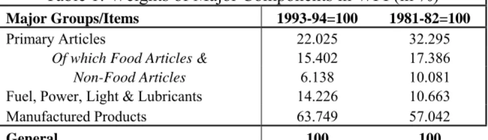
commodities in its commodity basket. Table 1 gives the broad weighting structure. WPI is available weekly; the lag is only two weeks for provisional index and ten weeks for the final index. It does not cover non-commodity producing sectors like services and other non-tradable goods.
Table 1: Weights of Major Components in WPI (in %)
Major Groups/Items 1993-94=100 1981-82=100
Primary Articles 22.025 32.295
Of which Food Articles & 15.402 17.386 Non-Food Articles 6.138 10.081
Fuel, Power, Light & Lubricants 14.226 10.663
Manufactured Products 63.749 57.042
General 100 100
Source: Ministry of Labour and Agarwal (2008)
Consumer price indices measure the cost of living as the changes in retail prices of selected goods and services on which a homogenous group of consumers spend the major part of their income. The consumer price index for industrial workers (CPI-IW) is compiled using retail prices collected from 261 markets in 76 centres. The items in the consumption basket in different centres vary from 120 to 160. Since January 2006, the revised CPI-IW series on new base-period of 2001 is available. This gives a higher weight to services but has a monthly frequency with a lag of two months.
Table 2 shows the weight of the six main commodity groups in the CPI-IW series. While CPI is constructed for specific centres and then aggregated to get the all-India index, WPI is computed on all-India basis. The commodity coverage in WPI is also wider than that in CPI.
WPI inflation averaged at around 5% per annum after 2000, only the component ‘Fuel, Power, Light and Lubricant (FPL&L)’ had an inflation rate of 10% per annum from 2000 to 2007. There is evidence of higher pass-through of international prices to domestic inflation. FPL&L inflation was the key driver of headline inflation after 2000 (Table 3).
7 This section draws on Agarwal (2008).
Table 2: Weights of Major Components in CPI-Industrial Workers (In %)
Groups/Items 1982=100 2001=100
Food 57 46.2
Pan, Supari, Tobacco & Intoxicants 3.15 2.27
Fuel & Light 6.28 6.43
Housing 8.67 15.27
Clothing, Bedding & Footwear 8.54 6.57 Miscellaneous Group (Services) 16.36 23.26
General 100 100
Source: Ministry of Labour and Agarwal (2008)
Table 3: Weighted Contribution in WPI by components
1981-85 1985-90 1990-95 1995-2000 2000-2007
Primary Articles 22.67 18.05 20.34 22.03 14.26
Food Articles 25.26 19.85 20.22 27.28 12.47
Non Food Articles 21.45 19.84 22.82 10.47 13.50
FPL&L 14.80 18.20 19.63 27.08 47.90
Manufactured Products 15.83 24.06 16.99 13.15 11.88
Note: Overall increase in WPI inflation is normalized to 100%, thus each column sums to 100 in the Table.
Source: RBI (2007) and Agarwal (2008)
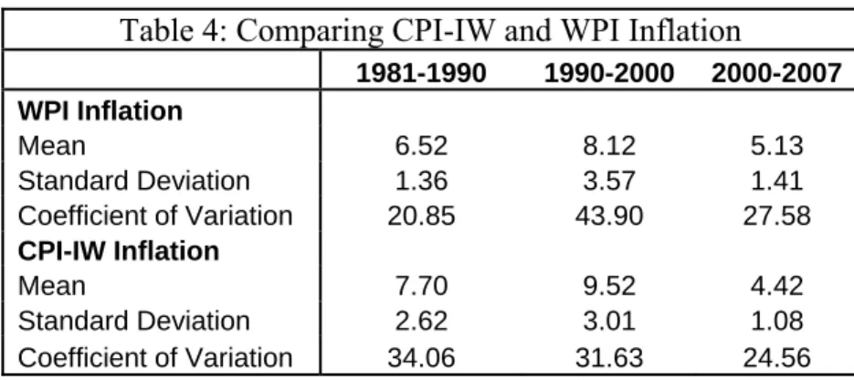
Table 4: Comparing CPI-IW and WPI Inflation
1981-1990 1990-2000 2000-2007 WPI Inflation Mean 6.52 8.12 5.13 Standard Deviation 1.36 3.57 1.41 Coefficient of Variation 20.85 43.90 27.58 CPI-IW Inflation Mean 7.70 9.52 4.42 Standard Deviation 2.62 3.01 1.08 Coefficient of Variation 34.06 31.63 24.56 Source: RBI (2007) and Agarwal (2008)
CPI-IW inflation averaged at around 7.6% from 1980 to 2007 (till March). It decelerated after 2000, coming down from 8.6% in late 1990s to 4.4% in the period 2000 to 2007. It was very volatile during 1980s (as measured by coefficient of variation) with volatility exceeding that of WPI inflation. Its volatility fell in the subsequent period before rising again in 1995 to 2000, but stayed below that of WPI. Since food group inflation has the highest weight in the CPI-IW inflation basket, its high volatility drove that of CPI-IW inflation.
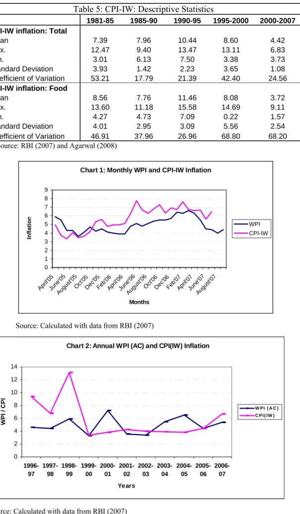
Table 5: CPI-IW: Descriptive Statistics
1981-85 1985-90 1990-95 1995-2000 2000-2007
CPI-IW inflation: Total
Mean 7.39 7.96 10.44 8.60 4.42
Max. 12.47 9.40 13.47 13.11 6.83
Min. 3.01 6.13 7.50 3.38 3.73
Standard Deviation 3.93 1.42 2.23 3.65 1.08
Coefficient of Variation 53.21 17.79 21.39 42.40 24.56
CPI-IW inflation: Food
Mean 8.56 7.76 11.46 8.08 3.72
Max. 13.60 11.18 15.58 14.69 9.11
Min. 4.27 4.73 7.09 0.22 1.57
Standard Deviation 4.01 2.95 3.09 5.56 2.54
Coefficient of Variation 46.91 37.96 26.96 68.80 68.20 Source: RBI (2007) and Agarwal (2008)
Chart 1: Monthly WPI and CPI-IW Inflation
0 1 2 3 4 5 6 7 8 9 Apri l'05 June'05 Augu st'05 Oct' 05 Dec '05 Feb'06Apri l'06 June'06 Augu st'06 Oct' 06 Dec '06 Feb'07Apri l'07 June'07 Augu st'07 Months Infla tio n WPI CPI-IW
Source: Calculated with data from RBI (2007)
Chart 2: Annual WPI (AC) and CPI(IW) Inflation
0 2 4 6 8 10 12 14 1996-97 1997-98 1998-99 1999-00 2000-01 2001-02 2002-03 2003-04 2004-05 2005-06 2006-07 Years WPI / CPI W PI ( A C ) C PI ( IW )
Chart 1, which maps Monthly WPI and CPI-IW for the period April 2005 to
September 2007, shows that although WPI inflation was less volatile, it led changes in CPI inflation. Oil shocks dominated in this period. The respective coefficients of variation were 17 and 23.
Chart 2 with annual data from the mid-nineties confirms the lead-lag pattern, and shows the changing volatility picture of the two series. WPI all commodities (AC) was more volatile in the period of oil price shocks and CPI-IW in the period of food price shocks. Cost-push factors have dominated Indian inflation in this period. In the late nineties, CPI inflation fell as food prices approached falling world prices and buffer stocks were large. The WPI inflation peak in 2001-02 coincided with the rise in oil prices. Table 3 shows industry's falling contribution to inflation, which indicates a rise in industrial productivity since the weight of manufacturing in WPI has risen from 57 to 64 in the current series with base 1993-94. Among components of demand, broad money growth was flat in the nineties. The fiscal deficit was large but since the government spends more on non-tradables, this and foreign inflows, should have raised non-tradable prices, but did not. In 1998-99, 2000-01, and in early 2003-04, inflation fell as supply shocks wore out, without a sharp tightening in monetary policy.
The international supply shocks, primarily international crude oil inflation, which drove WPI inflation in the current decade, have a lower weight in the CPI-IW basket than in the WPI basket. The alternative inflation rates do, however, tend to converge over long periods of time, as administered prices are changed, and CPI affects wages which raise costs for producers. The FPLL is the outright administered price
component in WPI inflation—this is only 14%, and part of it is no longer fixed after the APM was dismantled in 2002. Part of food items, weight 15.4%, is also
administered. In the CPI-IW the last category has a weight of 46.2%, fuel and light 6.43% and the services component (weight 23.3%) also has items with fixed user charges. Therefore the component subject to price intervention in WPI is about 30% compared to 60% for CPI-IW.
6. Simulations
The model is calibrated for the Indian economy following Goyal (2007, 2008). The earlier exercises established that if CPI is a function of lagged WPI and current change in exchange rates, targeting CPI inflation leads to high volatility and non-robust responses. Then, in response to both a cost shock affecting WPI and a generic natural interest rate shock, flexible DIT performs best. Flexible CIT (CPI inflation targeting) did almost as well under some kind of exchange rate management, which made the terms of trade credibly sticky.
The components of CPI and WPI shown in the section above, with the higher weight of administrative interventions on CPI, suggest that the lag structure used in the earlier simulations is indeed appropriate. The large delay in availability of CPI, and the larger share of volatile non-core components not affected by aggregate demand and therefore beyond the reach of the Central Bank, also suggest that domestic
inflation targeting is more appropriate in India at the present juncture. Oil shocks have a large effect on WPI, and food prices a large weight in the CPI. Administrative
interventions in food make the CPI adjust with a lag, and oil prices also affect food prices with a lag.
But the Indian macroeconomic scene is changing and so if it worth asking what happens if the lags affecting CPI reduce. This is the question we explore in the simulations below.
Consumer price inflation is now taken as a weighted average of current domestic prices and depreciation.
(
t t Ht)
t H t t H t H t H t t t P P 1;π , P , P , 1;π π , α e e 1 π , π = − − = − − = + − − −The policy response is obtained under discretion with a central bank minimizing different weighted averages of inflation (domestic or consumer), output and interest rate deviations from equilibrium values normalized at unity for the simulations
( 2 2 2 i q q y q
L= Y + ππ + i ). The weights attached to the different arguments of the loss
function (qs) ensure stability since the weight on inflation exceeds unity. Under strict inflation targeting only inflation has a positive weight of 2. The exchange rate directly affects consumer inflation while it affects domestic inflation through its affect on marginal cost. Monetary policy affects domestic inflation directly by changing the output gap; domestic inflation is a component of consumer inflation.
The calibration is loosely based on Indian stylized facts. Empirical estimations and the dominance of administered pricing in SOEME’s suggest that past inflation affects current inflation (Fraga et. al., 2004), so a modification of the AS Eq. (31) is made to accommodate such behaviour by imposing a share γb of lagged prices:
{
, 1}
ˆ , 1 1, t = f t H t+ + ′t + b H t− f + b =
H γ βE π λmc γ π γ γ
π
In most simulations γb is set at 0.2 so γf is 0.8. Because of less than perfectly flexible interest rates, lagged interest rate also enters the AD with a weight of 0.2. The openness coefficient α is set at 0.3; the proportion of R,8η at 0.4; β= 0.99 implies a riskless annual steady-state return of 4 percent; the price response to output, ϕ, is set at 0.25, which implies an average labour supply elasticity of 4. Consumption of the mature economy and of the rich is normalized at unity, five times that of the poor so CP = 0.2. Given η, this gives consistent C values of 0.75, K of 1.1 so that cP = -1.6 and ĸ=0.1. Initial conditions are normalized at unity so the log value is zero. The natural outputyt is derived from the flexible price equilibrium, with an employment subsidy ν =−log
(
1−τ)
set so as to correct for market power and for government temptation to change the terms of trade (GM, Section 4). In a SOEME it is also necessary to correct for the deviation from world income levels and poor infrastructure. Goyal (2008) derives the value of the subsidy as(
α)
κ δ μν = +log1− − +log . The index of infrastructure δ is taken as 0.5 less than the world level of unity. An elasticity of substitution between differentiated goods, ε
equal to 6, implies a steady-state mark-up, μ, of 1.2. The value of ν- μ derived from
8 GMM regressions of CPI inflation for India (Goyal, 2005) give a coefficient of expected inflation of 0.67. India’s share of imports in GDP was about 20 percent in 2005, and the proportion of population in rural areas 60 percent. In GMM regressions of aggregate demand with monthly data, the one period forward index of industrial production was strongly significant with a coefficient of –0.42.
the value of α, δ and ĸ is -0.9675. The price setting parameters are such that prices adjust in an average of one year (θ = 0.75), giving λ = 0.24.
Since σR = 1 and 1/σP=0, the implied average intertemporal elasticity of substitution is η(1-α) + α=0.58. A negative interest rate effect on consumption requires an intertemporal elasticity large enough so that the substitution effect is higher than the positive income effect of higher interest rates on net savers. Empirical studies have found real interest rates to have weak effects on consumption. Especially in low-income countries subsistence considerations are stronger than intertemporal factors. This is particularly so when the share of food in total expenditure is large. The elasticity Ogaki, Ostry and Reinhart (1996) estimate in a large cross-country study, varies from 0.05 for Uganda and Ethiopia to a high of 0.6 for Venezuela and Singapore. Our average elasticity compares well with these figures.
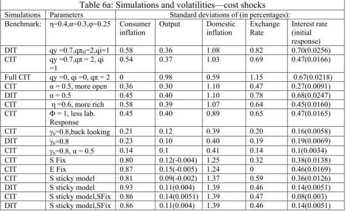
Burns (2008) estimates that the level of technology employed in developing countries is only one-fourth that in high income countries but technological progress increased 40-60 percent faster in the former than in the latter between the early 1990s and early 2000s. Since this catch-up has been even faster in India in recent years we take the value of at to be 0.8 in the SOEME when it is normalized at unity for the SOE. Table 6a reports the impulse responses to a calibrated 0.2 standard deviation cost shock to period one domestic inflation. The square of the unconditional standard deviations reported gives a measure of the welfare loss. The initial simulated variable value (in brackets) is also reported for selected simulations. Table 6a shows that now flexible CIT outperforms flexible DIT, giving lower volatilities despite a lower rise in the policy rate. The effective use of the direct exchange rate channel possible in this case reduces the necessity to contract output in response to the cost shock.
Sensitivity analysis with variation in key parameters using CIT as the benchmark has similar results as with DIT benchmark in Goyal (2007)(Table 6a and Figure 1). More openness and a higher proportion of R lower the initial interest response and
volatility, since the interest elasticity of output falls. The difference compared to DIT is a much larger reduction in the initial policy rate in a more open economy because of a larger impact of appreciation on CPI with higher α. There is a much greater reduction in CPI and exchange rate volatility in CIT compared to DIT even with the lower policy rate response under CIT. The effect of lower labour elasticity is muted under CIT with the policy rate unchanged until it starts falling slightly when ϕ = 1. In DIT the initial interest response first rises (at ϕ = 1)and then reduces as labour supply becomes even more inelastic (Goyal, 2007). These results are robust for different model structures. A SOE characterized by η=1 would therefore have a lower rise in interest rates and appreciation compared to a SOEME.
An aggressive response to inflation lowers the cost of disinflation and therefore volatilities because of the forward-looking behaviour modeled, and need not hold if this is moderated, since it is no longer so effective in anchoring inflation expectations. A simulation with γb=0.8, so that domestic inflation is backward looking, has a much smaller rise in interest rates. The response to and volatilities following a cost shock are muted. The performance is very similar to the benchmark DIT (Goyal, 2007). But
when lagged domestic inflation determined the CPI then there was a very large policy rate response under CIT even in this case since the cost shock raised the CPI and exchange rates being a forward looking component affecting CPI, the policy rate was raised to deliver a large appreciation. With both γb=0.8 and higher α, the large impact of the latter dominates.
Under exchange rate intervention, the loss of the effective exchange rate channel raises inflation volatility but lowers output volatility, compared to the benchmark, without much change in the policy rate. The clear advantage to a fixed exchange rate, which was there with DIT and lagged CPI, is no longer there. In the S sticky model, where S is credibly fixed, CIT output volatility is much lower, although inflation volatility exceeds the benchmark (Figure 2). DIT does better than CIT in this case, with a very low rise in the policy rate, a rise in output despite the cost shock, and inflation volatilities similar to CIT in the sticky S model. The conclusion is that fixed terms of trade can still lower output volatility in response to a cost shock, at the expense of slightly higher inflation volatility, but these advantages are to be gained more with DIT, compared to CIT. If reducing output volatility is a major objective, then fixed terms of trade and DIT still outperform CIT under a cost shock.
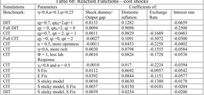
Table 6b reports the estimated reaction function coefficients of the predetermined variables in the different simulations. These continue to be intuitive, with a lower weight on the output gap and higher weight on inflation under the full targeting regimes. Since CPI inflation is itself a weighted average of domestic inflation and the exchange rate, the reaction function weights fall on these two respectively under CPI targeting. In the S sticky model the coefficient of the output gap and inflation both fall. The very low weight on output gap supports the flatter supply curve when S is fixed.
Table 6a: Simulations and volatilities—cost shocks Simulations Parameters Standard deviations of (in percentages): Benchmark: η=0.4,α=0.3,φ=0.25 Consumer inflation Output Domestic inflation Exchange Rate Interest rate (initial response) DIT qy =0.7,qπH=2,qi=1 0.58 0.36 1.08 0.82 0.70(0.0256) CIT qy =0.7,qπ = 2, qi =1 0.54 0.37 1.03 0.69 0.47(0.0166) Full CIT qy =0, qi =0, qπ = 2 0 0.98 0.59 1.15 0.67(0.0218)
CIT α = 0.5, more open 0.36 0.30 1.10 0.47 0.27(0.0091)
DIT α = 0.5 0.45 0.40 1.10 0.78 0.68(0.0247)
CIT η =0.6, more rich 0.58 0.39 1.07 0.64 0.45(0.0160)
CIT Φ = 1, less lab.
Response 0.45 0.40 0.89 0.65 0.47(0.0165)
CIT γb=0.8,back looking 0.21 0.12 0.39 0.20 0.16(0.0058)
DIT γb=0.8 0.23 0.10 0.40 0.19 0.19(0.0069)
CIT γb=0.8, α = 0.5 0.14 0.1 0.41 0.14 0.1(0.0034)
CIT S Fix 0.80 0.12(-0.004) 1.25 0.32 0.38(0.0138)
CIT E Fix 0.87 0.15(-0.005) 1.24 0 0.46(0.0169)
CIT S sticky model 0.81 0.09(-0.002) 1.37 0.59 0.36(0.0126) DIT S sticky model 0.93 0.11(0.004) 1.39 0.46 0.14(0.0051) CIT S sticky model,SFix 0.86 0.14(0.0051) 1.39 0.47 0.08(0.003) DIT S sticky model,SFix 0.86 0.11(0.004) 1.39 0.46 0.14(0.0051) Note: The bracketed terms give the value of the variable in the first period of the simulation
Table 6b: Reaction Functions—cost shocks
Simulations Parameters Coefficients of:
Benchmark: η=0.4,α=0.3,φ=0.25 Shock dummy/
Output gap Domestic inflation Exchange Rate Interest rate
DIT qy=0.7, qπH=2,qi=1 0.0133 0.1282 -0.0659
Full DIT qy = 0, qπH=2, qi = 0 0.0094 0.9098 -0.2500 CIT qy=0.7, qπ = 2, qi = 1 0.0011 0.0829 -0.1689 -0.0483 Full CIT qy =0, qi =0, qπ = 2 -0.0027 0.1091 -0.3072 -0.0300 CIT α = 0.5, more openness -0.0011 0.0453 -0.2258 -0.0402
CIT η=0.6, more rich 0.0020 0.0798 -0.1555 -0.0584
CIT Φ = 1, less lab. Response
0.0010 0.0826 -0.1728 -0.0538
CIT γb=0.8 and α = 0.5 -0.0010 0.017 -0.2224 -0.0394
CIT S Fix 0.0112 0.0692 -0.0957 -0.0542
CIT E Fix 0.0392 0.0844 -0.1151 -0.0577
CIT S sticky model 0.0010 0.0630 -0.1380 -0.0178
CIT S sticky model, S Fix 0.0037 0.0150 -0.0101 -0.0204
DIT S sticky model, S Fix 0.0039 0.0254 -0.0206
The dynamic impulse response as a calibrated 0.1 shock to the period one natural rate is given in Table 7a below. The generic response to a rise in the natural interest rate is a rise in the policy rate. But because initially the gap between the policy and the natural interest rate falls output rises, this raises domestic inflation, but the accompanying currency appreciation reduces consumer price inflation. The rise in the policy rate covers the expected future depreciation and slowly brings output back to steady-state levels. The response to a fall in natural rates to –0.01 is absolutely symmetric, with the signs reversed. Policy rates fall now.
Table 7a: Simulations and volatilities: natural interest rate shock
Simulations Parameters Standard deviations of (in percentages): Benchmark: η=0.4,α=0.3,φ=0.25 Consumer inflation Output Domestic inflation Exchange Rate Interest rate (initial response) DIT, 0.01rn qy=0.7, qπH=2,qi=1 0.46 0.16 0.31 1.60 0.39 (0.0133)
DIT, 0.01rn S Fix 0.31 0.16 0.31 1.02 0.39(0.0133)
DIT, 0.01rn E Fix 0.21 0.16(0.0061) 0.31 0.00 0.39 (0.0133) CIT, 0.01rn qy=0.7, qπ = 2, qi=1 0.19 0.28(0.0102) 0.27 1.00 0.20 (0.0011) CIT, .01rn S Fix 0.55 0.39(0.015) 0.62 1.84 0.46 (0.0112) CIT, .01rn E Fix 1.03 0.69(0.0251) 1.47(0.05) 0.00 1.17(0.0392)
DIT, .01rn S sticky model, S fix 0.12 0.32(0.011) 0.10 0.38 0.11(0.0039) CIT, .01rn S sticky model, 0.11 0.30(0.0107) 0.09(0.0026) 0.43 0.08(0.0010) CIT, .01rn S sticky model, S fix 0.12 0.33(0.0112) 0.10(0.0031) 0.38 0.11(0.0037) Note: The bracketed terms give the value of the variable in the first period of the simulation
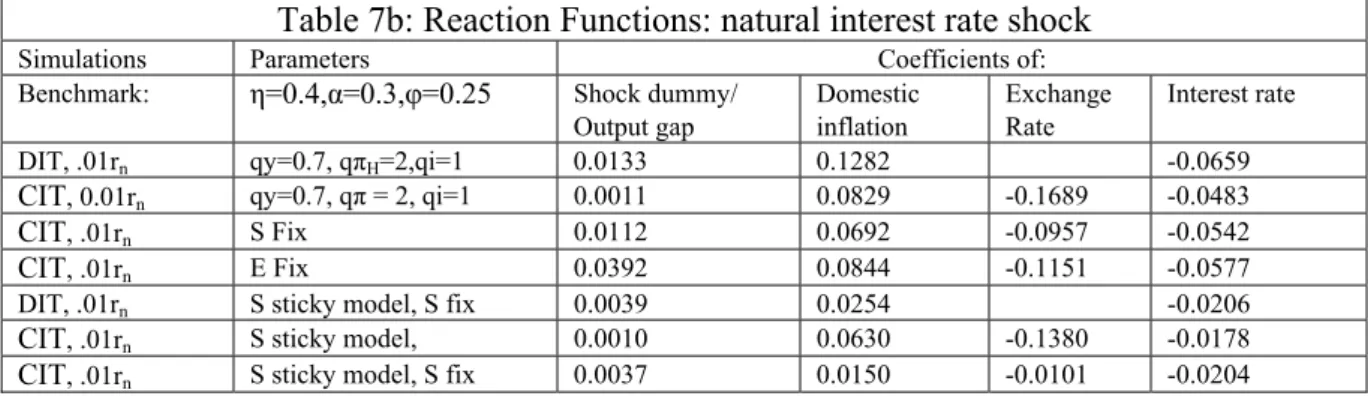
Since CIT acts largely through the direct exchange rate channel, the policy rate response is very low, implying large output volatility, even though inflation volatility remains lower than with DIT. Lagged CIT had a lower increase in policy rates but greater volatility in every other variable (Goyal, 2008). Output and inflation volatility is especially high when there is exchange rate intervention so that use of the exchange rate channel is limited (Figure 3). In the S sticky model, with S credibly fixed, the performance of DIT and CIT is almost identical. The familiar low coefficients for the policy reaction functions (Table 7b) again confirm the flatter supply curve with S fixed. So the conclusion is again that as long as there is some advantage to fixing S, flexible DIT remains the better form of inflation targeting.
Table 7b: Reaction Functions: natural interest rate shock
Simulations Parameters Coefficients of: Benchmark: η=0.4,α=0.3,φ=0.25 Shock dummy/
Output gap Domestic inflation Exchange Rate Interest rate DIT, .01rn qy=0.7, qπH=2,qi=1 0.0133 0.1282 -0.0659 CIT, 0.01rn qy=0.7, qπ = 2, qi=1 0.0011 0.0829 -0.1689 -0.0483
CIT, .01rn S Fix 0.0112 0.0692 -0.0957 -0.0542 CIT, .01rn E Fix 0.0392 0.0844 -0.1151 -0.0577
DIT, .01rn S sticky model, S fix 0.0039 0.0254 -0.0206 CIT, .01rn S sticky model, 0.0010 0.0630 -0.1380 -0.0178 CIT, .01rn S sticky model, S fix 0.0037 0.0150 -0.0101 -0.0204
7. Conclusion
The paper presents a simplified version of a basic microfoundations based small open economy model of the type used for monetary policy. Then the major differences in set-up and results due to two types of consumers and workers in an emerging market are set out. Dual or specific labour markets increase strategic complementarity so that there is a substantial effect of variations in nominal spending on output even if only some prices are sticky. But volatile terms of trade reduce this effect. So in a SOEME compared to a SOE the aggregate supply is flatter if the terms of trade are fixed. The AD is less interest elastic.
This result differs from earlier macroeconomic analysis for a developing economy (Rao, 1952) that pervasive supply bottlenecks could be expected to make demand stimuli ineffective. The difference arises because in an open economy supply bottlenecks are easier to alleviate. Moreover, in this class of models labour
productivity is the key output driver, and in labour-surplus economies established on catch-up growth path, capital is available to equip labour and raise its productivity. Goyal (2008) shows the distance between the subsistence consumption and mature consumption, raises potential output, but poor infrastructure and technological distance decrease it. The consumption factor dominates. Temporary shocks to subsistence consumption reduce the natural interest rate.
The key results from all the calibrations and simulations undertaken with the SOEME model are: Flexible DIT outperforms other kinds of targeting if there are lags in the CPI, otherwise flexible CIT is the best. But with terms of trade credibly fixed both are similar. Overall DIT is more robust—since CIT is volatile in some circumstances. So loss from information and time lags in CPI are minimal as long as exchange rate intervention is optimal. If domestic inflation is backward, not forward looking, a small policy rate response is optimal under flexible DIT and under CIT without lags in the CPI. If there are lags in the CPI, the policy rate becomes volatile.
As the economy becomes more open CIT becomes more effective, and therefore the loss from not being able to use it increases. It is necessary, despite India’s diversity, to develop an acceptable measure of average CPI and reduce the lags in its availability.
References
Agarwal A., 2008, ‘Inflation Targeting in India: An Explorative Analysis’, Chapter 1 in PhD thesis submitted to IGIDR.
Burns A., H. Timmer, E. Riordan, and W. Shaw, 2008, Global Economic Prospects 2008: Trends In Technology Diffusion in Developing Countries, World Bank Report, accessed from http://go.worldbank.org/TC26UFESJ0 on 16th January, 2008.
Clarida, R., Gali, J., and Gertler, M., 1999, ‘The Science of Monetary Policy: A New Keynesian perspective’, Journal of Economic Literature, 37 (4), 1661-707.
Clarida, R., Gali, J., and Gertler, M., 2001, ‘Optimal Monetary Policy in Closed Versus Open Economies: An integrated approach’, American Economic Review, 91
(2), May, 248-252.
Fraga, A., I. Goldfajn, and A. Minella, 2004, ‘Inflation Targeting in Emerging Market Economies’, in Gertler M. and K. Rogoff (eds.) NBER Macroeconomics Annual, Cambridge: MIT Press.
Gali, J. and T. Monacelli, 2005, “Monetary Policy and Exchange Rate Volatility in a Small Open Economy.” Review of Economic Studies, 72(3): 707-734.
Goyal, A., 2008, ‘The Natural Interest rate in Emerging Markets,’ IGIDR working paper.
Goyal, A., 2007, ‘A General Equilibrium Open Economy Model for Emerging Markets,’ paper presented at ISI International Conference on Comparative Development, available at
http://www.isid.ac.in/~planning/ComparativeDevelopmentConference.html. An earlier version is available as IGIDR working paper WP-2007-016.
Goyal, A., 2005, ‘Incentives from Exchange rates in an Institutional Context,’ IGIDR working paper available at www.igidr.ac.in/pdf/publication/WP-2005-002-R1.pdf, forthcoming Journal of Quantitative Economics.
Obstfeld, M. and K. Rogoff, 1996, Foundations of International Macroeconomics,
Cambridge, Massachusetts: MIT Press.
Ogaki, Masao, Jonathan Ostry, and Carmen M. Reinhart, 1996, ‘Savings Behaviour in Low-and Middle-Income Countries: A comparison’, IMF Staff Papers 43 (March):
38-71
Rao, V.K.R.V, 1952, ‘Investment, Income and the Multiplier in an Underdeveloped Economy’, The Indian Economic Review, February, reprinted in Agarwala, A.N. and
S.P. Singh (eds.) The Economics of Underdevelopment, London, Oxford, New York:
Oxford University Press, 205-218, 1958.
Svensson, L.E.O, 2000, ‘Open-economy inflation targeting’, Journal of International Economics, 50, 155-183.
Woodford, M, 2003, Interest and prices: Foundations of a Theory of Monetary Policy, NJ: Princeton University Press.
Appendix
To derive the aggregate demand supply equality
The allocation of foreign consumption to goods produced in the SOEME is the same as FOC (11) with P*t C*t instead of Pt Ct Multiplying and dividing by P*F,t and converting the numerator P*F,t into SOEME prices using the nominal exchange rate gives: * * , * , * , * , t t F t t H t F t H C P P P P C =αε
Of the two relative prices, the first one compares the price of SOEME goods to all other foreign goods translated into SOEME prices. The second relative price
compares the foreign country price index to the price index of all other foreign goods. Thus more SOEME goods are imported as a function of these two relative prices, the weight of foreign goods in the consumption basket, and aggregate foreign
consumption.
Multiplying and dividing by Pt and substituting Qt: * , * , t t H t t t H C P P Q C =α
Substituting the FOC for the SOEME consumer (10) and that just derived for the foreign consumer, in the aggregate demand = supply Eq. (18) for the SOEME (Yt =CH,t +CH,t*), gives:
(
)
* , , 1 t t H t t t H t t t C P P Q P C P Y = −α +α Substituting out * tC using risk sharing Eq. (17):
(
α)
α σ1 , , 1 − + − = CQ P P Q P C P Y t t H t t t H t t tSimplifying and assuming σ =1 gives:
) ( 1 1 , σ − = C Q P P Y t t H t t σ α 1−1 =S C Q Ct t t t t S C Y = α (19)