Practical application of simplex method for solving linear programming problems

(1)

BALKAN JOURNAL

OF APPLIED MATHEMATICS

AND INFORMATICS

(BJAMI)

GOCE DELCEV UNIVERSITY - STIP, REPUBLIC OF MACEDONIA

FACULTY OF COMPUTER SCIENCE

ISSN 2545-479X print ISSN 2545-4803 on line

(2)

BALKAN JOURNAL

OF APPLIED MATHEMATICS

AND INFORMATICS

(BJAMI)

GOCE DELCEV UNIVERSITY - STIP, REPUBLIC OF MACEDONIA

FACULTY OF COMPUTER SCIENCE

ISSN 2545-479X print ISSN 2545-4803 on line

(3)

Managing editor Biljana Zlatanovska Ph.D. Editor in chief Zoran Zdravev Ph.D. Technical editor Slave Dimitrov

Address of the editorial office Goce Delcev University – Stip Faculty of philology Krste Misirkov 10-A PO box 201, 2000 Štip, R. of Macedonia

AIMS AND SCOPE:

BJAMI publishes original research articles in the areas of applied mathematics and informatics.

Topics:

1. Computer science;

2. Computer and software engineering; 3. Information technology;

4. Computer security; 5. Electrical engineering; 6. Telecommunication;

7. Mathematics and its applications;

8. Articles of interdisciplinary of computer and information sciences with education, economics, environmental, health, and engineering.

BALKAN JOURNAL

OF APPLIED MATHEMATICS AND INFORMATICS (BJAMI), Vol 1

ISSN 2545-479X print ISSN 2545-4803 on line Vol. 1, No. 1, Year 2018

(4)

EDITORIAL BOARD

Adelina Plamenova Aleksieva-Petrova, Technical University – Sofia, Faculty of Computer Systems and Control, Sofia, Bulgaria

Lyudmila Stoyanova, Technical University - Sofia , Faculty of computer systems and control, Department – Programming and computer technologies, Bulgaria

Zlatko Georgiev Varbanov, Department of Mathematics and Informatics, Veliko Tarnovo University, Bulgaria

Snezana Scepanovic, Faculty for Information Technology, University “Mediterranean”, Podgorica, Montenegro

Daniela Veleva Minkovska, Faculty of Computer Systems and Technologies, Technical University, Sofia, Bulgaria

Stefka Hristova Bouyuklieva, Department of Algebra and Geometry, Faculty of Mathematics and Informatics, Veliko Tarnovo University, Bulgaria

Vesselin Velichkov, University of Luxembourg, Faculty of Sciences, Technology and Communication (FSTC), Luxembourg

Isabel Maria Baltazar Simões de Carvalho, Instituto Superior Técnico, Technical University of Lisbon, Portugal

Predrag S. Stanimirović, University of Niš, Faculty of Sciences and Mathematics, Department of Mathematics and Informatics, Niš, Serbia

Shcherbacov Victor, Institute of Mathematics and Computer Science, Academy of Sciences of Moldova, Moldova

Pedro Ricardo Morais Inácio, Department of Computer Science, Universidade da Beira Interior, Portugal

Sanja Panovska, GFZ German Research Centre for Geosciences, Germany Georgi Tuparov, Technical University of Sofia Bulgaria

Dijana Karuovic, Tehnical Faculty “Mihajlo Pupin”, Zrenjanin, Serbia Ivanka Georgieva, South-West University, Blagoevgrad, Bulgaria

Georgi Stojanov, Computer Science, Mathematics, and Environmental Science Department The American University of Paris, France

Iliya Guerguiev Bouyukliev, Institute of Mathematics and Informatics, Bulgarian Academy of Sciences, Bulgaria

Riste Škrekovski, FAMNIT, University of Primorska, Koper, Slovenia

Stela Zhelezova, Institute of Mathematics and Informatics, Bulgarian Academy of Sciences, Bulgaria Katerina Taskova, Computational Biology and Data Mining Group,

Faculty of Biology, Johannes Gutenberg-Universität Mainz (JGU), Mainz, Germany. Dragana Glušac, Tehnical Faculty “Mihajlo Pupin”, Zrenjanin, Serbia Cveta Martinovska-Bande, Faculty of Computer Science, UGD, Macedonia

Blagoj Delipetrov, Faculty of Computer Science, UGD, Macedonia Zoran Zdravev, Faculty of Computer Science, UGD, Macedonia Aleksandra Mileva, Faculty of Computer Science, UGD, Macedonia

Igor Stojanovik, Faculty of Computer Science, UGD, Macedonia Saso Koceski, Faculty of Computer Science, UGD, Macedonia Natasa Koceska, Faculty of Computer Science, UGD, Macedonia Aleksandar Krstev, Faculty of Computer Science, UGD, Macedonia Biljana Zlatanovska, Faculty of Computer Science, UGD, Macedonia

Natasa Stojkovik, Faculty of Computer Science, UGD, Macedonia Done Stojanov, Faculty of Computer Science, UGD, Macedonia Limonka Koceva Lazarova, Faculty of Computer Science, UGD, Macedonia Tatjana Atanasova Pacemska, Faculty of Electrical Engineering, UGD, Macedonia

(5)

(6)

5

C O N T E N T

Aleksandar, Velinov, Vlado, Gicev

PRACTICAL APPLICATION OF SIMPLEX METHOD FOR SOLVING

LINEAR PROGRAMMING PROBLEMS ... 7 Biserka Petrovska , Igor Stojanovic , Tatjana Atanasova Pachemska

CLASSIFICATION OF SMALL DATA SETS OF IMAGES WITH

TRANSFER LEARNING IN CONVOLUTIONAL NEURAL NETWORKS ... 17 Done Stojanov

WEB SERVICE BASED GENOMIC DATA RETRIEVAL ... 25 Aleksandra Mileva, Vesna Dimitrova

SOME GENERALIZATIONS OF RECURSIVE DERIVATES

OF k-ary OPERATIONS ... 31 Diana Kirilova Nedelcheva

SOME FIXED POINT RESULTS FOR CONTRACTION

SET - VALUED MAPPINGS IN CONE METRIC SPACES ... 39 Aleksandar Krstev, Dejan Krstev, Boris Krstev, Sladzana Velinovska

DATA ANALYSIS AND STRUCTURAL EQUATION MODELLING

FOR DIRECT FOREIGN INVESTMENT FROM LOCAL POPULATION ... 49 Maja Srebrenova Miteva, Limonka Koceva Lazarova

NOTION FOR CONNECTEDNESS AND PATH CONNECTEDNESS IN

SOME TYPE OF TOPOLOGICAL SPACES ... 55 The Appendix

Aleksandra Stojanova , Mirjana Kocaleva , Natasha Stojkovikj , Dusan Bikov , Marija Ljubenovska , Savetka Zdravevska , Biljana Zlatanovska , Marija Miteva , Limonka Koceva Lazarova

OPTIMIZATION MODELS FOR SHEDULING IN KINDERGARTEN

AND HEALTHCARE CENTES ... 65 Maja Kukuseva Paneva, Biljana Citkuseva Dimitrovska, Jasmina Veta Buralieva,

Elena Karamazova, Tatjana Atanasova Pacemska

PROPOSED QUEUING MODEL M/M/3 WITH INFINITE WAITING

LINE IN A SUPERMARKET ... 73 Maja Mijajlovikj1, Sara Srebrenkoska, Marija Chekerovska, Svetlana Risteska,

Vineta Srebrenkoska

APPLICATION OF TAGUCHI METHOD IN PRODUCTION OF SAMPLES

PREDICTING PROPERTIES OF POLYMER COMPOSITES ... 79 Sara Srebrenkoska, Silvana Zhezhova, Sanja Risteski, Marija Chekerovska

Vineta Srebrenkoska Svetlana Risteska

APPLICATION OF FACTORIAL EXPERIMENTAL DESIGN IN

PREDICTING PROPERTIES OF POLYMER COMPOSITES ... 85 Igor Dimovski, Ice Gjumandeloski, Filip Kochoski, Mahendra Paipuri,

Milena Veneva , Aleksandra Risteska

COMPUTER AIDED (FILAMENT WINDING) TAPE PLACEMENT

(7)

PRACTICAL APPLICATION OF SIMPLEX METHOD FOR SOLVING LINEAR

PROGRAMMING PROBLEMS

Aleksandar, Velinov1_{, Vlado, Gicev} 1

1_{Faculty of Computer Science, Goce Delcev University, Stip, Macedonia}

[email protected] [email protected]

Abstract: In this paper we consider application of linear programming in solving optimization problems with constraints. We used the simplex method for finding a maximum of an objective function. This method is applied to a real example. We used the “linprog” function in MatLab for problem solving. We have shown, how to apply simplex method on a real world problem, and to solve it using linear programming. Finally we investigate the complexity of the method via variation of the computer time versus the number of control variables.

Keywords: simplex method, linear programming, objective function, complexity.

1. Introduction

Linear programming was developed during World War II, when a system with which to maximize the efficiency of resources was of utmost importance. New war-related projects demanded optimization of constrained resources. “Programming” was used as a military term that referred to activities such as planning schedules efficiently or deploying men optimally [1].

Mathematical programming is that branch of mathematics dealing with techniques for maximizing or minimizing an objective function subject to linear, nonlinear, and integer constraints on the variables. Special case of mathematical programming is a linear programming.Linear programming is concerned with the maximization or minimization of a linear objective function with many variables subject to linear equality and inequality constraints [2]. Linear programming can be viewed as a part of a great revolutionary development. It has the ability to define general goals and to find detailed decisions in order to achieve that goals. It can be faced with practical situations of great complexity. To formulate real-world problems, linear programming uses mathematical terms (models), techniques for solving the models (algorithms), and engines for executing the steps of algorithms (computers and software) [3].

Optimization principles have important aspect in modern engineering design and system operations in various areas. Computers capable of solving large-scale problems contribute to the recent development of new optimization techniques. The main goal of these techniques is to optimize (maximize or minimize) some function f. This functions are called objective functions. As a case study we used the objective function f that represent the revenue of the production of electronic elements, more precisely graphics cards. We used methods for maximizing the revenue of the company. Using linear programming, we can model wide variety of objective functions as: yield per minute in a chemical process, revenue in a production of cars, the hourly number of customers served in a bank, the mileage per gallon of a certain type of car, the production of computers on monthly basis and so on. Sometimes we may want to minimize f if f is the cost per unit of producing certain graphics cards (opposite of our example where we maximize the revenue of production), the operating cost of some power plant, the time needed to produce a new type of car, the daily loss of heat in a heating system, the costs for IT infrastructure in some company and so on.

In most optimization problems the objective function f depends on several variables:

x1, x2,…..xn

These variables are called “control variables” because we can control them, that is, we can choose their values. For example the production of some plant may depend on temperature x1, moisture content x2, nitrogen in the soil x3. The

efficiency of a certain air-conditioning system may depend on air pressure x1, temperature x2, cross-sectional area of

(8)

7

PRACTICAL APPLICATION OF SIMPLEX METHOD FOR SOLVING LINEAR

PROGRAMMING PROBLEMS

Aleksandar, Velinov1_{, Vlado, Gicev} 1

1_{Faculty of Computer Science, Goce Delcev University, Stip, Macedonia}

[email protected] [email protected]

Abstract: In this paper we consider application of linear programming in solving optimization problems with constraints. We used the simplex method for finding a maximum of an objective function. This method is applied to a real example. We used the “linprog” function in MatLab for problem solving. We have shown, how to apply simplex method on a real world problem, and to solve it using linear programming. Finally we investigate the complexity of the method via variation of the computer time versus the number of control variables.

Keywords: simplex method, linear programming, objective function, complexity.

1. Introduction

Linear programming was developed during World War II, when a system with which to maximize the efficiency of resources was of utmost importance. New war-related projects demanded optimization of constrained resources. “Programming” was used as a military term that referred to activities such as planning schedules efficiently or deploying men optimally [1].

Mathematical programming is that branch of mathematics dealing with techniques for maximizing or minimizing an objective function subject to linear, nonlinear, and integer constraints on the variables. Special case of mathematical programming is a linear programming.Linear programming is concerned with the maximization or minimization of a linear objective function with many variables subject to linear equality and inequality constraints [2]. Linear programming can be viewed as a part of a great revolutionary development. It has the ability to define general goals and to find detailed decisions in order to achieve that goals. It can be faced with practical situations of great complexity. To formulate real-world problems, linear programming uses mathematical terms (models), techniques for solving the models (algorithms), and engines for executing the steps of algorithms (computers and software) [3].

Optimization principles have important aspect in modern engineering design and system operations in various areas. Computers capable of solving large-scale problems contribute to the recent development of new optimization techniques. The main goal of these techniques is to optimize (maximize or minimize) some function f. This functions are called objective functions. As a case study we used the objective function f that represent the revenue of the production of electronic elements, more precisely graphics cards. We used methods for maximizing the revenue of the company. Using linear programming, we can model wide variety of objective functions as: yield per minute in a chemical process, revenue in a production of cars, the hourly number of customers served in a bank, the mileage per gallon of a certain type of car, the production of computers on monthly basis and so on. Sometimes we may want to minimize f if f is the cost per unit of producing certain graphics cards (opposite of our example where we maximize the revenue of production), the operating cost of some power plant, the time needed to produce a new type of car, the daily loss of heat in a heating system, the costs for IT infrastructure in some company and so on.

In most optimization problems the objective function f depends on several variables:

x1, x2,…..xn

These variables are called “control variables” because we can control them, that is, we can choose their values. For example the production of some plant may depend on temperature x1, moisture content x2, nitrogen in the soil x3. The

efficiency of a certain air-conditioning system may depend on air pressure x1, temperature x2, cross-sectional area of

outlet x3, moisture content x4, and so on. The optimization theory develops methods for optimal choices of x1,…,xn,

UDK: 519.852

(9)

8

which maximize or minimize the objective function f, that is, methods for finding optimal values of x1,…,xn. In many

problems the choice of values of x1,…,xn depends on some constraints. Those are restrictions that arise from the nature

of the problem and variables. When we determine the optimal values of control variables we must take into account those limitations. In our example the constraints refer to the number of graphics cards produced in a period of one hour, if we use four different machines in production. There are a lot of examples for constraints in a real world problems that can be solved with linear programming such as: if x1 is a production cost, then x1≥0, and there are many

other variables (time, weight, distance traveled by salesmen) that can take nonnegative values only. In this example the constraints have the form of inequalities. Constraints can also have the form of equations. In this paper we consider the optimization problem with constraints.

In linear programming the objective function is a linear function given as: z=f(x1,…,xn) =a1x1 + a2x2 + …+ anxn

We can rearrange the structure that characterizes linear programming problems (perhaps after several manipulations) into the following form [1]:

Maximize c1x1 + c2x2 + · · · + cnxn = z

Subject to a11x1 + a12x2 + · · · + a1nxn = b1

a21x1 + a22x2 + · · · + a2nxn = b2

am1x1 + am2x2 + · · · + amnxn = bm

x1, x2, . . . , xn ≥ 0

The part after “Maximize” represent the objective function, and the part after “Subject to” represent the constraints. This is a normal form of the linear programming problem. Here x1,…,xn include also the slack variables. That are auxiliary variables for which the c’s in f are zero. We use the slack variables to convert inequalities to equations. For example if the objective function is:

f=60x1+40x2

And the constraints are:

2x1+3x2≤80

5x1+4x2≤80

x1≥0

x2≥0

The normal form of the linear programming problem would be:

f-60x1-40x2 = 0

2x1+3x2+x3 =80

5x1+4x2+ x4 =80

As we said before x1 and x2 are called control variables or decision variables while x3 and x4 are slack variables or

auxiliary variables. A set of x1, x2 . . . xn satisfying all the constraints is called a feasible point and the set of all such

points is called the feasible region. The solution of the linear program must be a point (x1, x2, . . . , xn) in the feasible

region, otherwise not all the constraints would be satisfied. Linear programming algorithm find a point in feasible region, if there exist, on which the objective function has maximum (or minimum) value [4]. This is a feasible solution.

… … … …

A feasible solution is called an optimal solution if for it the objective function f becomes maximum, compared with the values of f at all feasible solutions. Basic feasible solution is a feasible solution for which at least n-m of variables x1, x2 . . . xn are zero.

There are two methods for solving linear programming problems: Graphical method and simplex method. The graphical method is limited to linear programming problems involving two decision variables and a limited number of constraints due to the difficulty of graphing and evaluating more than two decision variables. This restriction severely limits the use of the graphical method for real-world problems. The graphical method is simple and easy to understand and it is a very good learning tool. The simplex method is much more powerful than the graphical method and provides the optimal solution to LP problems containing thousands of decision variables and constraints. It uses an iterative algorithm to solve for the optimal solution. Moreover, the simplex method provides information on slack variables (unused resources) and shadow prices (opportunity costs) that is useful in performing sensitivity analysis [5]. Because our real problem involve four decision variables we used the simplex method. We used it instead of graphical method due to the difficulty of graphing.

2. Simplex method

As we said before, for solving linear programming problems with two variables, the graphical solution method is convenient. For problems involving more than two variables or problems involving a large number of constraints, an algorithm should be tailored to computers. One such method is developed by George Dantzig in 1946, and it is called simplex method. This method provides a systematic way of examining the vertices of the feasible region to determine the optimal value of the objective function [6]. It is an iterative method. In this method, one proceeds stepwise from one basic feasible solution to another in such a way that the objective function f always increases. In previous example the objective function was:

f=60x1+40x2

We used a normal form to transform linear inequalities to equations. In this conversion we introduced two slack variables x3 and x4. The normal form of the objective function and the constraints were presented earlier. In this normal

form x1≥0,…, x4≥0. Normal form contains linear system of equations. To find an optimal solution, we may consider its augmented matrix:

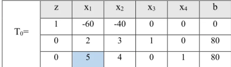
Table 1: Initial simplex table

T0=

z x1 x2 x3 x4 b

1 -60 -40 0 0 0

0 2 3 1 0 80

0 5 4 0 1 80

This matrix is called a simplex table or simplex tableau. T0 is the initial simplex table. This table contains two types

of variables: basic variables and non-basic variables. By basic variables we mean those whose columns contain only one nonzero entry. In our example basic variables are x3, x4 and x1, x2 are non-basic variables. From the simplex table

we can get a basic feasible solution. We obtain it by setting the non-basic variables to zero. The basic feasible solution is:

x1=0, x2=0, x3=80/1=80, x4=80/1=80, z=0;

We get the values for x3 and x4 when we divide b with x3 and b with x4. We use pivoting to obtain the optimal solution.

It is designed to take us to the basic feasible solution with higher and higher values of z until the maximum of z is reached. In this example x1,…,x4 are restricted to nonnegative values.

Step 1a: Selection of the Column of the pivot

We select as a column of the pivot the first column with a negative entry in row 1. In T0 it is a Column 2. Aleksandar Velinov, Vlado Gicev

(10)

9 which maximize or minimize the objective function f, that is, methods for finding optimal values of x1,…,xn. In many

problems the choice of values of x1,…,xn depends on some constraints. Those are restrictions that arise from the nature

of the problem and variables. When we determine the optimal values of control variables we must take into account those limitations. In our example the constraints refer to the number of graphics cards produced in a period of one hour, if we use four different machines in production. There are a lot of examples for constraints in a real world problems that can be solved with linear programming such as: if x1 is a production cost, then x1≥0, and there are many

other variables (time, weight, distance traveled by salesmen) that can take nonnegative values only. In this example the constraints have the form of inequalities. Constraints can also have the form of equations. In this paper we consider the optimization problem with constraints.

In linear programming the objective function is a linear function given as: z=f(x1,…,xn) =a1x1 + a2x2 + …+ anxn

We can rearrange the structure that characterizes linear programming problems (perhaps after several manipulations) into the following form [1]:

Maximize c1x1 + c2x2 + · · · + cnxn = z

Subject to a11x1 + a12x2 + · · · + a1nxn = b1

a21x1 + a22x2 + · · · + a2nxn = b2

am1x1 + am2x2 + · · · + amnxn = bm

x1, x2, . . . , xn ≥ 0

The part after “Maximize” represent the objective function, and the part after “Subject to” represent the constraints. This is a normal form of the linear programming problem. Here x1,…,xn include also the slack variables. That are auxiliary variables for which the c’s in f are zero. We use the slack variables to convert inequalities to equations. For example if the objective function is:

f=60x1+40x2

And the constraints are:

2x1+3x2≤80

5x1+4x2≤80

x1≥0

x2≥0

The normal form of the linear programming problem would be:

f-60x1-40x2 = 0

2x1+3x2+x3 =80

5x1+4x2+ x4 =80

As we said before x1 and x2 are called control variables or decision variables while x3 and x4 are slack variables or

auxiliary variables. A set of x1, x2 . . . xn satisfying all the constraints is called a feasible point and the set of all such

points is called the feasible region. The solution of the linear program must be a point (x1, x2, . . . , xn) in the feasible

region, otherwise not all the constraints would be satisfied. Linear programming algorithm find a point in feasible region, if there exist, on which the objective function has maximum (or minimum) value [4]. This is a feasible solution.

… … … …

A feasible solution is called an optimal solution if for it the objective function f becomes maximum, compared with the values of f at all feasible solutions. Basic feasible solution is a feasible solution for which at least n-m of variables x1, x2 . . . xn are zero.

There are two methods for solving linear programming problems: Graphical method and simplex method. The graphical method is limited to linear programming problems involving two decision variables and a limited number of constraints due to the difficulty of graphing and evaluating more than two decision variables. This restriction severely limits the use of the graphical method for real-world problems. The graphical method is simple and easy to understand and it is a very good learning tool. The simplex method is much more powerful than the graphical method and provides the optimal solution to LP problems containing thousands of decision variables and constraints. It uses an iterative algorithm to solve for the optimal solution. Moreover, the simplex method provides information on slack variables (unused resources) and shadow prices (opportunity costs) that is useful in performing sensitivity analysis [5]. Because our real problem involve four decision variables we used the simplex method. We used it instead of graphical method due to the difficulty of graphing.

2. Simplex method

As we said before, for solving linear programming problems with two variables, the graphical solution method is convenient. For problems involving more than two variables or problems involving a large number of constraints, an algorithm should be tailored to computers. One such method is developed by George Dantzig in 1946, and it is called simplex method. This method provides a systematic way of examining the vertices of the feasible region to determine the optimal value of the objective function [6]. It is an iterative method. In this method, one proceeds stepwise from one basic feasible solution to another in such a way that the objective function f always increases. In previous example the objective function was:

f=60x1+40x2

We used a normal form to transform linear inequalities to equations. In this conversion we introduced two slack variables x3 and x4. The normal form of the objective function and the constraints were presented earlier. In this normal

form x1≥0,…, x4≥0. Normal form contains linear system of equations. To find an optimal solution, we may consider its augmented matrix:

Table 1: Initial simplex table

T0=

z x1 x2 x3 x4 b

1 -60 -40 0 0 0

0 2 3 1 0 80

0 5 4 0 1 80

This matrix is called a simplex table or simplex tableau. T0 is the initial simplex table. This table contains two types

of variables: basic variables and non-basic variables. By basic variables we mean those whose columns contain only one nonzero entry. In our example basic variables are x3, x4 and x1, x2 are non-basic variables. From the simplex table

we can get a basic feasible solution. We obtain it by setting the non-basic variables to zero. The basic feasible solution is:

x1=0, x2=0, x3=80/1=80, x4=80/1=80, z=0;

We get the values for x3 and x4 when we divide b with x3 and b with x4. We use pivoting to obtain the optimal solution.

It is designed to take us to the basic feasible solution with higher and higher values of z until the maximum of z is reached. In this example x1,…,x4 are restricted to nonnegative values.

We select as a column of the pivot the first column with a negative entry in row 1. In T0 it is a Column 2.

(11)

10 Step 2a: Selection of the Row of the pivot

We divide the values from b in the Row 2 and Row 3 with the corresponding entries of the column selected as pivot column (80/2 and 80/5). The row of the pivot will be the row with the smallest quotient. In our example the pivot will be 5 because 80/5 is smallest (80/5<80/2). If the rows in the pivot column have a non-positive values, we do not compute a ratio b/x1 and we do not take this quotient into account when deciding about the row of the pivot [7].

Step 3a: Elimination by Row operations

We use elimination by row operation to make zeros the values above and below the pivot. For that we use Gauss-Jordan method [8]. After row operation we have a new matrix determined by the values obtained from executed operations. The new matrix will be:

Table 2: Simplex table T1 after elimination

T1=

z x1 x2 x3 x4 b

1 0 8 0 12 960 Row1+12*Row3 0 0 7/5 1 -2/5 48 _2/5*Row3

Row2-0 5 4 0 1 80

Now we can see that basic variables are x1 and x3, and non-basic variables are x2 and x4. The basic feasible solution

given by T1 is [9]:

x1=80/5=16, x2=0, x3=48/1=48, x4=0, z=960;

Because T1 contains no more negative entries in Row 1, this is a basic feasible solution. We can conclude that z=f(16,0)=60*16+40*0=960 is the maximum possible value. This is the solution of our problem by the simplex method of linear programming.

3. Numerical Example

We apply simplex method on a linear programming problem and we solve it. Our problem is:

The company for production of electronic chips produces 4 types of graphics cards (C1, C2, C3, C4), that are produced from 4 types of machines (M1, M2, M3 and M4). The M1 machine produces the C1 graphics card for 1 min, C2 for 2 min, C3 for 3 min, and the graphics card C4 for 2 min. The M2 machine produces a C1 graphics card for 3 min, C2 for 2 min, C3 for 4 min and C4 for 6 min. The M3 machine produces the C1 graphics card for 2 min, C2 for 1 min, C3 for 3 min and C4 for 3 min. The M4 machine produces a C1 graphics card for 2 min, C2 for 4 min, C3 for 3 min and C4 for 5 min. The C1 graphics card is sold for $20, C2 for $35, C3 for $40 and C4 for $50. Determine the number of graphics cards (x1 for C1, x2 for C2, x3 for C3, and x4 for C4) which maximizes the revenue generated from the

production of graphics cards for an hour.

The number of graphics cards x1, x2, x3, and x4 must be nonnegative. Hence the objective function (to be maximized)

and the eight constraints are:

Objective function: z=20x1+35x2+40x3+50x4 M1: 1x1+2x2+3x3+2x4<=60 M2: 3x1+2x2+4x3+6x4<=60 M3: 2x1+1x2+3x3+3x4<=60 M4: 2x1+4x2+3x3+5x4<=60 x1≥0 x2≥0 x3≥0 x4≥0

4. Algorithm

The normal form of the linear programming problem is:

z-20x1-35x2-40x3-50x4 = 0

1x1+2x2+3x3+2x4+ x5 =60

3x1+2x2+4x3+6x4+ + x6 =60

2x1+1x2+3x3+3x4+ + +x7 =60

2x1+4x2+3x3+5x4+ + + +x8 =60

The initial simplex table T0 is:

Table 3: Initial simplex table for our LP problem

T0= z x1 x2 x3 x4 x5 x6 x7 x8 b 1 20 35 40 50 0 0 0 0 0 0 1 2 3 2 1 0 0 0 60 0 3 2 4 6 0 1 0 0 60 0 2 1 3 3 0 0 1 0 60 0 2 4 3 5 0 0 0 1 60

We select as a column of the pivot the first column with a negative entry in row 1. We used positive values in Row 1. They correspond to the negative values from objective function. In T0 it is a Column 2 (Value -20).

Step 2a: Selection of the Row of the pivot

We divide the values from b in the Row 2 and Row 3 with the corresponding entries of the column selected as pivot column (60/1, 60/3, 60/2, 60/2). The row of the pivot will be the row with the smallest quotient. In our example the pivot will be 3 because 60/3 is the smallest quotient (Row 3).

With elimination by row operation we got a new simplex table T1: Table 4: Simplex table after first row elimination

T1= z x1 x2 x3 x4 x5 x6 x7 x8 b 1 0 21.6 13.3 10 0 -6.67 0 0 -400 _20/3*Row3 Row1-0 0 1.33 1.67 0 1 -0.33 0 0 40 _1/3*Row3 Row2-0 1 0.67 1.33 2 0 0.33 0 0 20 Row3/Pivot 0 0 -0.33 0.33 -1 0 -0.67 1 0 20 _2/3*Row3 Row4-0 0 2.67 0.33 1 0 -0.67 0 1 20 _2/3*Row3 Row5-In the Row 3 we used the quotient Row3/Pivot. It is a difference between this approach and the method described in the Part 2 of this paper. The difference is also the Row 1 where we used positive values instead of negative values in Part 2 (negative values at the end). The new pivot is 2.67.

We repeated the steps from 1a to 3a and after the row eliminations we got the other simplex tables (Table 5 and Table 6).

(12)

11 Step 2a: Selection of the Row of the pivot

We divide the values from b in the Row 2 and Row 3 with the corresponding entries of the column selected as pivot column (80/2 and 80/5). The row of the pivot will be the row with the smallest quotient. In our example the pivot will be 5 because 80/5 is smallest (80/5<80/2). If the rows in the pivot column have a non-positive values, we do not compute a ratio b/x1 and we do not take this quotient into account when deciding about the row of the pivot [7].

We use elimination by row operation to make zeros the values above and below the pivot. For that we use Gauss-Jordan method [8]. After row operation we have a new matrix determined by the values obtained from executed operations. The new matrix will be:

Table 2: Simplex table T1 after elimination

T1=

z x1 x2 x3 x4 b

1 0 8 0 12 960 Row1+12*Row3 0 0 7/5 1 -2/5 48 _2/5*Row3

Row2-0 5 4 0 1 80

Now we can see that basic variables are x1 and x3, and non-basic variables are x2 and x4. The basic feasible solution

given by T1 is [9]:

x1=80/5=16, x2=0, x3=48/1=48, x4=0, z=960;

Because T1 contains no more negative entries in Row 1, this is a basic feasible solution. We can conclude that z=f(16,0)=60*16+40*0=960 is the maximum possible value. This is the solution of our problem by the simplex method of linear programming.

3. Numerical Example

We apply simplex method on a linear programming problem and we solve it. Our problem is:

The company for production of electronic chips produces 4 types of graphics cards (C1, C2, C3, C4), that are produced from 4 types of machines (M1, M2, M3 and M4). The M1 machine produces the C1 graphics card for 1 min, C2 for 2 min, C3 for 3 min, and the graphics card C4 for 2 min. The M2 machine produces a C1 graphics card for 3 min, C2 for 2 min, C3 for 4 min and C4 for 6 min. The M3 machine produces the C1 graphics card for 2 min, C2 for 1 min, C3 for 3 min and C4 for 3 min. The M4 machine produces a C1 graphics card for 2 min, C2 for 4 min, C3 for 3 min and C4 for 5 min. The C1 graphics card is sold for $20, C2 for $35, C3 for $40 and C4 for $50. Determine the number of graphics cards (x1 for C1, x2 for C2, x3 for C3, and x4 for C4) which maximizes the revenue generated from the

production of graphics cards for an hour.

The number of graphics cards x1, x2, x3, and x4 must be nonnegative. Hence the objective function (to be maximized)

and the eight constraints are:

Objective function: z=20x1+35x2+40x3+50x4 M1: 1x1+2x2+3x3+2x4<=60 M2: 3x1+2x2+4x3+6x4<=60 M3: 2x1+1x2+3x3+3x4<=60 M4: 2x1+4x2+3x3+5x4<=60 x1≥0 x2≥0 x3≥0 x4≥0

4. Algorithm

The normal form of the linear programming problem is:

z-20x1-35x2-40x3-50x4 = 0

1x1+2x2+3x3+2x4+ x5 =60

3x1+2x2+4x3+6x4+ + x6 =60

2x1+1x2+3x3+3x4+ + +x7 =60

2x1+4x2+3x3+5x4+ + + +x8 =60

The initial simplex table T0 is:

Table 3: Initial simplex table for our LP problem

T0= z x1 x2 x3 x4 x5 x6 x7 x8 b 1 20 35 40 50 0 0 0 0 0 0 1 2 3 2 1 0 0 0 60 0 3 2 4 6 0 1 0 0 60 0 2 1 3 3 0 0 1 0 60 0 2 4 3 5 0 0 0 1 60

We select as a column of the pivot the first column with a negative entry in row 1. We used positive values in Row 1. They correspond to the negative values from objective function. In T0 it is a Column 2 (Value -20).

Step 2a: Selection of the Row of the pivot

We divide the values from b in the Row 2 and Row 3 with the corresponding entries of the column selected as pivot column (60/1, 60/3, 60/2, 60/2). The row of the pivot will be the row with the smallest quotient. In our example the pivot will be 3 because 60/3 is the smallest quotient (Row 3).

With elimination by row operation we got a new simplex table T1: Table 4: Simplex table after first row elimination

T1= z x1 x2 x3 x4 x5 x6 x7 x8 b 1 0 21.6 13.3 10 0 -6.67 0 0 -400 _20/3*Row3 Row1-0 0 1.33 1.67 0 1 -0.33 0 0 40 _1/3*Row3 Row2-0 1 0.67 1.33 2 0 0.33 0 0 20 Row3/Pivot 0 0 -0.33 0.33 -1 0 -0.67 1 0 20 _2/3*Row3 Row4-0 0 2.67 0.33 1 0 -0.67 0 1 20 _2/3*Row3 Row5-In the Row 3 we used the quotient Row3/Pivot. It is a difference between this approach and the method described in the Part 2 of this paper. The difference is also the Row 1 where we used positive values instead of negative values in Part 2 (negative values at the end). The new pivot is 2.67.

We repeated the steps from 1a to 3a and after the row eliminations we got the other simplex tables (Table 5 and Table 6).

(13)

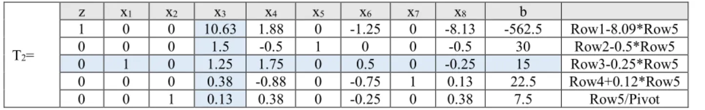
12 Table 5: Simplex table after second row elimination

T2= z x1 x2 x3 x4 x5 x6 x7 x8 b 1 0 0 10.63 1.88 0 -1.25 0 -8.13 -562.5 Row1-8.09*Row5 0 0 0 1.5 -0.5 1 0 0 -0.5 30 Row2-0.5*Row5 0 1 0 1.25 1.75 0 0.5 0 -0.25 15 Row3-0.25*Row5 0 0 0 0.38 -0.88 0 -0.75 1 0.13 22.5 Row4+0.12*Row5 0 0 1 0.13 0.38 0 -0.25 0 0.38 7.5 Row5/Pivot Table 6: Final simplex table

T3= z x1 x2 x3 x4 x5 x6 x7 x8 b 1 -8.5 0 0 -13 0 -5.5 0 -6 -690 _8.5*Row5 Row1-0 -1.2 0 0 -2.6 1 -0.6 0 -0.2 12 _1.2*Row3 Row2-0 0.8 0 1 1.4 0 0.4 0 -0.2 12 Row3/Pivot 0 -0.3 0 0 -1.4 0 -0.9 1 0.2 18 _0.304*Row3 Row4-0 -0.1 1 0 0.2 0 -0.3 0 0.4 6 _0.104*Row3

Row5-5.

Implementation in Matlab

As we can see in the solution (T3 simplex table), Row 1 contains no more positive entries in Row 1. We can see that now x2, x3, x5 and x7 are basic variables and x1, x4, x6, x8 are non-basic variables. Hence the basic feasible solution

is:

x1=0, x2=6/1=6, x3=12/1=12, x4=0, x5=12/1=12, x6=0, x7=18/1=18, x8=0

The maximum possible revenue is 690 because z = f(0,6,12,0)=20*0+35*6+40*12+50*0=690. The company will have maximum profit for one hour if it produces 6 graphics cards from type C2 and 12 graphics cards from type C3. We also used the MATLAB tool to find the solution of our linear programming problem. We used the “linprog” function [10].

This is the MATLAB code:

>> f=[-20 -35 -40 -50] f = -20 -35 -40 -50 >> A=[1 2 3 2; 3 2 4 6; 2 1 3 3; 2 4 3 5] A = 1 2 3 2 3 2 4 6 2 1 3 3 2 4 3 5 >> b=[60 60 60 60] b = 60 60 60 60 >> Aeq=[] Aeq = [] >> beq=[] beq = [] >> lb=[0 0 0 0] lb = 0 0 0 0 >> ub=[] ub = [] >> [X,Z]=linprog(f,A,b,Aeq,beq,lb,ub) Optimization terminated. X = 0.0000 6.0000 12.0000 0.0000 Z = -690.0000 Here the “linprog function” has some parameters:

• f – the linear objective function vector

• A – the matrix of the linear inequality constraints

• b - the matrix of the linear inequality constraints

• Aeq - the matrix of the linear equality constraints

• beq - the right-hand side vector of the linear equality constraints

• lb - the vector of the lower bounds

• ub - the vector of the upper bounds

(14)

13 Table 5: Simplex table after second row elimination

T2= z x1 x2 x3 x4 x5 x6 x7 x8 b 1 0 0 10.63 1.88 0 -1.25 0 -8.13 -562.5 Row1-8.09*Row5 0 0 0 1.5 -0.5 1 0 0 -0.5 30 Row2-0.5*Row5 0 1 0 1.25 1.75 0 0.5 0 -0.25 15 Row3-0.25*Row5 0 0 0 0.38 -0.88 0 -0.75 1 0.13 22.5 Row4+0.12*Row5 0 0 1 0.13 0.38 0 -0.25 0 0.38 7.5 Row5/Pivot Table 6: Final simplex table

T3= z x1 x2 x3 x4 x5 x6 x7 x8 b 1 -8.5 0 0 -13 0 -5.5 0 -6 -690 _8.5*Row5 Row1-0 -1.2 0 0 -2.6 1 -0.6 0 -0.2 12 _1.2*Row3 Row2-0 0.8 0 1 1.4 0 0.4 0 -0.2 12 Row3/Pivot 0 -0.3 0 0 -1.4 0 -0.9 1 0.2 18 _0.304*Row3 Row4-0 -0.1 1 0 0.2 0 -0.3 0 0.4 6 _0.104*Row3

Row5-5.

Implementation in Matlab

As we can see in the solution (T3 simplex table), Row 1 contains no more positive entries in Row 1. We can see that now x2, x3, x5 and x7 are basic variables and x1, x4, x6, x8 are non-basic variables. Hence the basic feasible solution

is:

x1=0, x2=6/1=6, x3=12/1=12, x4=0, x5=12/1=12, x6=0, x7=18/1=18, x8=0

The maximum possible revenue is 690 because z = f(0,6,12,0)=20*0+35*6+40*12+50*0=690. The company will have maximum profit for one hour if it produces 6 graphics cards from type C2 and 12 graphics cards from type C3. We also used the MATLAB tool to find the solution of our linear programming problem. We used the “linprog” function [10].

This is the MATLAB code:

>> f=[-20 -35 -40 -50] f = -20 -35 -40 -50 >> A=[1 2 3 2; 3 2 4 6; 2 1 3 3; 2 4 3 5] A = 1 2 3 2 3 2 4 6 2 1 3 3 2 4 3 5 >> b=[60 60 60 60] b = 60 60 60 60 >> Aeq=[] Aeq = [] >> beq=[] beq = [] >> lb=[0 0 0 0] lb = 0 0 0 0 >> ub=[] ub = [] >> [X,Z]=linprog(f,A,b,Aeq,beq,lb,ub) Optimization terminated. X = 0.0000 6.0000 12.0000 0.0000 Z = -690.0000 Here the “linprog function” has some parameters:

• f – the linear objective function vector

• A – the matrix of the linear inequality constraints

• b - the matrix of the linear inequality constraints

• Aeq - the matrix of the linear equality constraints

• beq - the right-hand side vector of the linear equality constraints

• lb - the vector of the lower bounds

• ub - the vector of the upper bounds

(15)

14

Figure 1. Dependency between the number of control variables and computer time

6. Order of complexity of the method

Using the “tic/toc” method on “linprog” function in MatLab, we got the dependency between the number of control variables and computer time. We used different number of variables (from 50 to 300 with step 50). We can see from Figure 1 that the execution time (computer time) increases with increasing the number of control variables as exponential function.

7. Conclusion

Linear programming is an optimization technique that is used for obtaining the most optimal solution for a real world problem. We represent the problem with a mathematical model which involves an objective function and linear inequalities. There are two methods for solving linear programming problems: Graphical method and simplex method. Simplex method provides a systematic way of examining the vertices of the feasible region to determine the optimal value of the objective function. The “linprog” function in MatLab can be used to solve linear programming problems. The execution time of this function increases with increasing the number of control variables.

References:

[1] Whitman College. Linear Programming: Theory and Applications.

https://www.whitman.edu/Documents/Academics/Mathematics/lewis.pdf

[2] Dantzig, G.B, Thapa, M.N (1997). Linear programming 1: Introduction: Springer-Verlag New York, LLC, book

[3] Bioinformatics Research Group, Advanced Computing Research Laboratory. Linear programming.

http://bioinfo.ict.ac.cn/~dbu/AlgorithmCourses/Lectures/Dantzig2002.pdf

[4] Carnegie Mellon University, School of Computer Science. Linear programming. http://www.cs.cmu.edu/~ravishan/adv-alg/Lecture12.pdf

[5] Brock University. Linear Programming: The Graphical and Simplex Methods. http://spartan.ac.brocku.ca/~pscarbrough/scarb-alp-burch/Chapters%201-24-16.htm [6] Cengage. Linear programming.The simplex method: Maximization.

http://college.cengage.com/mathematics/larson/elementary_linear/4e/shared/downloads/c09s3.pdf

[7] The University of Texas at Dallas. The Simplex Method in Tabular Form.

https://www.utdallas.edu/~scniu/OPRE-6201/documents/LP06-Simplex-Tableau.pdf

[8] Adenegan, K.E, Aluko, T.M (2012). Gauss and gauss-jordan elimination methods for solving system of linear equations: comparisons and applications: Journal of Science and Science Education, Ondo Vol. 3(1), pp. 97 – 105.

[9] Luenberger, G.D, Ye, Y. (2008). Linear and Nonlinear Programming: Springer Science and Business Media, LLC, book.

[10]Ploskas, N, Samaras, N. (2017). Linear Programming Using MATLAB: S Springer International Publishing AG, book.

(16)

15 Figure 1. Dependency between the number of control variables and computer time