A Two-Sample Non-Parametric Likelihood Ratio Test

Discussion Papers in Economics

No. 2000/62

Dynamics of Output Growth, Consumption and Physical Capital

in Two-Sector Models of Endogenous Growth

by

Farhad Nili

Department of Economics and Related Studies University of York

No. 2005/25

A Two-Sample Non-Parametric Likelihood Ratio Test

by

A Two-Sample Non-Parametric Likelihood Ratio

Test

1

Patrick Marsh

Department of Economics

University of York

Heslington, York

YO10 5DD

tel. +44 1904 433084

fax +44 1904 433759

e-mail: [email protected]

July 26, 2005

1_{Thanks are due to Francesco Bravo, Giovanni Forchini, Les Godfrey, Grant Hillier,}

Abstract

This paper proposes a test for the hypothesis that two samples have the same distri-bution. The likelihood ratio test of Portnoy (1988) is applied in the context of the consistent series density estimator of Crain (1974) and Barron and Sheu (1991). It is proven that the test, when suitably standardised, is asymptotically standard normal and consistent against any complementary alternative. In comparison with the es-tablished Kolmogorov-Smirnov and Cramér-von Mises procedures the proposed test enjoys broadly comparable finite sample size properties, but vastly superior power properties.

1

Introduction

The problem of testing whether two independent samples are drawn from the same distribution is ubiquitous in applied statistics. Statistical tests for the two-sample hy-pothesis are commonly adaptations of tests that an identically and independently dis-tributed sample has a particular, known, distribution. Examples are the Kolmogorov-Smirnov and Cramér-von Mises procedures, see Darling (1957) for detailed exposition in the single sample case and Kiefer (1959) for multi-sample extensions. A fuller ac-count of these and other procedures can be found in Conover (1999).

This paper instead derives a test for the two-sample problem based upon the goodness of fit tests of Marsh (2005) and Claeskens and Hjort (2004). Those tests, although differing in terms of how the null hypothesis is imposed, are essentially the likelihood ratio test of Portnoy (1988), made non-parametric via the consistent exponential series density estimator of Crain (1974, 1976 & 1977) and Barron and Sheu (1991). Consequently it is relatively straightforward to establish the necessary asymptotic properties;first that the test, when appropriately standardised, is asymp-totically standard normal and second that it is consistent against any complimentary alternative.

Of concern in applied research, for any suggested procedure, are three things; whether implementation is intuitive and straightforward, whether empirically relevant critical values (i.e. having actual size close to nominal) are readily available and whether the test offers power against theoretically relevant alternatives.

In terms of implementation, the Kolmogorov-Smirnov and Cramér-von Mises are based upon criteria utilising the sup and L2 norms on the space of distributions.

In particular the Cramér-von Mises has appeal, see Anderson (1962), in that the resultant test can be written entirely in terms of the respective ranks of observations from the two samples within a pooled sample. The proposed test is instead based upon the Kullback-Leibler (Entropy) distance, on the space of densities. Specifically,

it is directly related to a likelihood ratio test for a simple hypothesis in the (albeit infinite) exponential family. In addition, as will be exposed below, the form of the statistic actually only depends upon the estimated parameters in that family and the raw moments of the samples themselves. In practice the proposed test involves only testing a simple hypothesis in the exponential family, with only the dimension of that family to be determined. Following Marsh (2005) the data driven selection criteria of both Akaike (1974) and Schwarz (1978) may be easily applied. Either criterion delivers test which is relatively straightforward to implement.

Regarding the availability of critical values, for the two-sample Cramér-von Mises procedure, Anderson (1962) provides a numerical approximation, while Kim (1969) provides an asymptotic distribution function for the Kolmogorov-Smirnov procedure. Although theoretically critical values may instead be found through simulation, hav-ing empirically relevant tabulated values is more convenient for applied problems. The proposed likelihood ratio statistic, when not standardised with respect to its degrees of freedom is asymptotically square. Critical values from standard Chi-square tables are shown, in this paper, to havefinite sample numerical properties not dissimilar to those tabulated for the established tests. Further numerical evidence involving comparisons of these two established procedures while others can be found in Burr (1964) and Dufour and Farhat (2002).

Since all of these tests are distribution free, and hence critical values could be directly simulated, albeit at considerable numerical cost, we must consider numerical performance under the alternative. Power is examined by considering alternatives in which the samples have distributions differing in terms of their moments. Excepting the case of different means, where the performance is comparable, the proposed non-parametric likelihood ratio test has significantly more power. For certain alternatives involving distributions with different variances, skewness or kurtosis the proposed test may be as much as four or even five times more powerful than either of the established procedures.

The plan for the rest of the paper is as follows, the next section provides the main definitions and results for both the density estimator and the asymptotics for the resultant two-sample non-parametric likelihood ratio test. Section 3 details the numerical experiments of the paper and is followed by brief conclusions. An appendix contains the proof of the theorem containing the asymptotic results as well as tables containing the numerical results.

2

A Two-Sample Likelihood Ratio Test

Let _{Xi} nX

i=1 and {Yi} nY

i=1 be i.i.d. samples taken from the random variables X and

Y respectively, having common sample space _R. Let F(τ) = Pr[X _≤ τ] and G(τ) = Pr[Y _≤τ], and suppose we wish to test

H0 :F(τ) =G(τ) for allτ ∈R,

against any complimentary alternative. In order to apply the likelihood ratio test of Portnoy (1988) in this context we will employ the exponential series density estimator

first employed by Crain (1974, 1976 and 1977) and extended by Barron and Sheu (1991).

To proceed define the monotone function h(τ) :_R→(₋a, a), a <_∞, so that

xi =h(Xi) and yi =h(Yi),

or generically x = h(X) and y = h(Y) and denote their density functions as px(h)

and py(h), respectively. The null hypothesis implies that px(h) = py(h) = p(h). Let

φj(h), j = 1, ..., m be a set of linearly independent functions spanning (−a, a) then

according to Barron and Sheu (1991) the exponential series estimator forp(h)is the maximum likelihood estimator (mle) in the family

ph(θ) = exp ( _m X j=1 θjφj(h)−ψm(θ) ) , (1)

where θ= (θ1, ...,θm)0 and the cumulant function is defined by ψm(θ) = ln Z a −a exp ( _m X j=1 θjφj(h) ) dh. (2)

Details on the implementation of the estimator may be found in Marsh (2005). To proceed, given samples _{xi}

nX

i=1 and {yi}

nY

i=1 define the following vectors inR

m ˆ θx : Ra −aφj(h)ph(ˆθx)dh= 1 nX PnX i=1φj(xi) ˆ θy : Ra −aφj(h)ph(ˆθy)dh= 1 nY PnY i=1φj(yi) θ0x : Ra −aφj(h)ph(θ0x)dh = Ra −aφj(h)px(h)dh θ0y : Ra −aφj(h)ph(θ0y)dh = Ra −aφj(h)py(h)dh                                      j = 1, .., m, (3)

and define the Sobolev space of functions, W2r, so that f(x) ∈ W2r if the (r−1)th

derivative off(.) is absolutely continuous and therth _{derivative is square integrable.}

The pertinent results of Crain (1973, 1974 and 1976) and Barron and Sheu (1991) can be summarized in the following lemma:

Lemma 1 Let ln(p(h))_∈Wr

2 with r≥2 and suppose that as nX, nY and m→ ∞,

nX nY =O(1) and m 3 nX =o(1), then:

(i) For all nX, nY and m, θˆx and θˆy exist and are unique and as m → ∞, θ0x and

θ0y exist and are unique.

(ii) Let D(p1|p2)denote the Kullback-Leibler divergence then

D(ph(θ0x)|px(h)) = Or ¡ m−2r¢ D ³ ph(ˆθx)|px(h) ´ = Op µ m nX +m−2r ¶ ,

and similarly for D³ph(ˆθy)|p(h)

´

.

(iii) Let_|._| be Euclidean distance in_Rm, then_|θˆx−θ0x|,|θˆy−θ0y| areOp

³p

m/nX

´

.

The importance of the set of results comprising Lemma 1 is that we can asymp-totically approximate the densitiespx(h)andpy(h)byph(θ0x)andph(θ0y). Moreover,

since θ0x andθ0y are the unique solutions to lines 3 and 4 of (3) then the two-sample

hypothesis can (asymptotically inm) be reformulated as

lim

m→∞ H ∗

0 :θ0x =θ0y vs. H1 :θ0x6=θ0y. (4)

Consequently, the test statistic can be formulated in terms of likelihood ratio tests for the (asymptotically) simple hypothesis θ0x = θ0y in the exponential family (1).

That is, rather than being based upon either the sup or L2 norms on distributions

of the Kolmogorov-Smirnov and Cramér-von Mises procedures, here we exploit the Kullback-Leibler (relative entropy) distance on densities.

The crucial asymptotic results required for the two-sample case follow almost trivially from the single sample. First, notice that under the null hypothesis (4) and via the triangle inequality

|θˆx−θˆy|≤|θˆx−θˆx0|+|θˆy−θˆx0|=Op µr m nX ¶ , (5)

while given the additivity of the Kullback-Leibler divergence

D³ph(ˆθx)|ph(ˆθy) ´ =Op µ m nX +m−2r ¶ . (6) In order to test H∗

0 in (4) define, for a sampleh1, .., hn,

p_θˆ(h) =p_θˆ(h1, .., hn) = lim m,n→∞, m3_/n→0θsup ∈Rm exp ( _m X j=1 θj n X i=1 φj(hi)−nψm(θ) ) . (7)

Thus we can write a likelihood ratio

Λh_θ1,θ2 = ln µ pθ1(h) pθ2(h) ¶ ,

which is, implicitly, a test for the simple null hypothesis θ =θ1 against θ =θ2 using

a sample of sizen onh. From this can define our two-sample likelihood ratio test,

Λx,y_θˆ x,θˆy =Λ x ˆ θx,θˆy+Λ y ˆ θx,ˆθy = ln à p_θˆ_x(x) p_θˆ_y(x) ! + ln à p_θˆ_y ¡ y¢ p_θˆ_x ¡ y¢ ! . (8)

Alternatively, in terms of Portnoy’s (1988) test we can further decompose so that

Λx,y_θˆ x,θˆy = ln µ_p ˆ θx(x) pθ0(x) ¶ + ln à pθ0(x) p_θˆ_y(x) ! + ln à p_θˆ_y ¡ y¢ pθ0 ¡ y¢ ! + ln à pθ0 ¡ y¢ p_θˆ_x ¡ y¢ ! , (9)

where under the null;θ0 =θ0x =θ0y.That is the decomposition of the likelihood ratio

in (9) implies that the test can be interpreted as the sum of four likelihood ratios for testing the two hypotheses; θ0x = θ0 and θ0y = θ0 using both of the samples on X

andY.

Formally we will reject H∗

0 :θ0x =θ0y in favour of H1 :θ0x 6=θ0y if

Λ_θx,y_ˆ

x,θˆy > k, (10)

where k is a suitably chosen critical value. As mentioned in the introduction, there is a relative dearth of distributional results for nonparametric two-sample tests, par-ticularly in comparison with their one sample counterparts. Therefore the following Theorem demonstrates that a standardised version of the test is asymptotically stan-dard normal underH∗

0 and that under H1 the test is consistent.

Theorem 1 (i) Let

λnX,nY = Λx,y_θˆ x,θˆy−m √ m , then λnX,nY →dN(0,1),

(ii) define kα by Pr[N[0,1]> kα|H0] =α>0, then Pr[λX,Y > kα|H1]→1, as nX, nY &m → ∞ and m3/nX →0.

In summary, Theorem 1 establishes the necessary asymptotic theory for the two-sample test. Specifically, and unlike current tests, we have a standard asymptotic distribution under the null. Moreover consistency follows, almost trivially, from the properties of likelihood ratio tests in the exponential family.

Implementation of the test is particularly straightforward. From (7) we have

Λx_θˆ x,θˆy =nX ·³ ˆ θx−θˆy ´0 ¯ x₋³ψm(ˆθx)−ψm(ˆθy) ´¸ ,

and similarly for Λy_θˆ

x,θˆy, so that from (8), we obtain Λx,y_θˆ x,θˆy =nX ·³ ˆ θx−θˆy ´0 (¯x− nY nX ¯ y)−(1− nY nX ) ³ ψm(ˆθx)−ψm(ˆθy) ´¸ .

Moreover, in the interesting special case of nX =nY the standardised test simplifies

as λn = nX ³ ˆ θx−θˆy ´0 (¯x₋y¯)₋m √ m →dN(0,1), as m, nX → ∞ and m3/nX →0.

3

Numerical Analysis

Theorem 1 demonstrates that asymptotically and under the null hypothesis λnX,nY

is standard normal. In practice, in order for the asymptotic normal distribution to serve as a reliable approximation m must be large. This implies a large number of estimating equations in (3) and hence the potential is for the whole process to become infeasible. Specifically, other experiments involving the single sample version of the Portnoy (1988) test, which will not be reported here, suggest that it is only for values of m above 15 with sample sizes above 500 that the standard normal provides an acceptable approximation. Instead, as in Portnoy (1988), we can instead utilise the asymptotic relation Λm = 2Λ x,y ˆ θx,θˆy →dχ 2 (2m), (11)

as nX, nY &m → ∞ and m3/nX → 0. That is the Chi-square may be used as a

distributional approximation and, as will be demonstrated numerically, provides a reasonable approximation to the finite sample distribution of Λm.

More important than the choice of asymptotic benchmark will be how to choose the dimension of the model, m. Since the likelihood ratios into which the statistic

Λx,y_θˆ

x,θˆy may be partitioned are all likelihood ratio statistics for testing simple

hypothe-ses in the exponential well established data driven selection criteria may be employed. Specifically, here we will use both the Akaike (1974) information criterion (AIC) as well as the Bayesian information criterion (BIC) of Schwarz (1978). To implement these, define the set of integers _M =_{1,2, ...,m¯_}, and let the estimated dimensions based upon these criteria bemˆA andmˆB, respectively, then they satisfy

ˆ mA = arg max m∈M h LX(ˆθx) +LY(ˆθy)−2m i ˆ mB = arg max m∈M h LX(ˆθx) +LY(ˆθy)−mln(nXnY) i , (12) where LX(ˆθx) = nX X i=1 m X k=1 (ˆθx)kφk(xi)−nXψm ³ ˆ θx ´ LY(ˆθy) = nY X i=1 m X k=1 (ˆθy)kφk(yi)−nYψm ³ ˆ θy ´ .

Notice that the criteria in (12) impose a common dimension on the estimators for both samples. It would be possible to optimise separately, however this would merely introduce an unnecessary complication in terms of using the chi-square distribution as an approximation. In any case, since both LX(θ) = O(nX) and LY(θ) = O(nY)

for allθ,then

asnX,m¯ → ∞ ,m¯3/nX →0 ˆ mA→ ∞ ˆ mB → ∞ .

That is if we allow m¯ to grow slowly relative tonX then both criteria will deliver a

consistent density estimator for each sample. We shall denote the two resulting test statistics asΛmˆA for that based upon the AIC andΛmˆB for that based upon the BIC.

The numerical properties of ΛmˆA and ΛmˆB will be compared with those of the

two-sample version of the Kolmogorov-Smirnov and Cramér—von Mises tests, defined in our notation by KS = r nXnY nX+nY sup i | FnX(xi)−GnY(yi)|, (13) CM = nXnY (nX+nY)2 "_n X X i=1 (FnX(xi)−FnX(yi)) 2₊ nY X i=1 (GnY(yi)−GnY(xi)) 2 # ,

where FnX(.) and GnY(.) are the empirical distribution functions of the samples

ob-tained fromX and Y respectively. Although these are not the only two-sample tests currently available, they do enjoy the advantage of having relatively well understood asymptotic distributions. For theKS test from Kim (1969) as nX, nY → ∞ then

Pr[KS _≤s]_→G(s) = 1₋2

∞

X

r=1

(₋1)r−1e−2r2s2 ; s >0.

Asymptotic critical values of nominal size α can be obtained via solution forcKS

α of α= 2 k X r=1 (₋1)r−1e−2r2(cKSα ) 2 ,

and to 4 decimal places wefind

cKS0.05 = 1.358 ; cv

KS

0.1 = 1.220.

Also from Anderson (1962) CM has the same asymptotic distribution as the single sample Cramér—von Mises test, as tabulated in Anderson and Darling (1952). Thus for the CM test we have asymptotic critical values

cCM_0.05 = 0.4614 ; cv₀CM_.1 = 0.3473.

Asymptotic critical values for anyΛm test saycvαm,are obtained fromPr[χ2m ≤cvαm] =

1₋α.

The first set of three experiments concern the finite sample performance of the asymptotic critical values as approximations to the finite sample distribution. For

the purposes all of the experiments to follow the set M = _{3,4,5_} was optimised over to construct both the ΛmˆA and ΛmˆB tests, for sample sizes of nX =nY = n=

50,100,200,400.All of the experiments are based upon5000Monte Carlo replications. All computations were performed on a Pentium IV 3.0GHz P.C. running Mathematica 4.0. A single replication of all 4 statistics took between 1 and 2 seconds, depending upon the sample size.

The first experiment consisted of generating samples _{Xi}ni=1 and {Yi}ni=1 from

X _∼Y _∼N(0,1), and then samples_{xi}in=1 and {yi}ni=1 lying in (0,1)via

xi = 3 p Φ(Xi) ; yi = 3 p Φ(Yi) (14)

where Φ(.) is the standard normal CDF. The second experiment used the standard exponential distribution, i.e. X _∼ Y _∼ Exp[1], with then the Exponential CDF replacing the standard normal in (14). Lastly, the third experiment varies the set up slightly, in that we assume that _{Xi}ni=1 and{Yi}ni=1 are generated from

X _∼Y _∼    N(₋1,1) with prob. 0.5 N(1,1) with prob. 0.5 ,

and now xi =F(Xi) whereF(.) is the CDF of a N(0,2) random variable, theyi are

defined similarly.

Deliberately neitherxi noryi are constructed to have the uniform distribution on

(0,1). The reason, as Marsh (2005) highlights, is that for the selection criteria for the likelihood ratio tests cannot be consistent, since the uniform is embedded within the exponential with m = 0 and _M cannot contain 0. For the tests based upon the empirical distribution functions this issue is irrelevant.

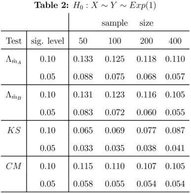
The Monte Carlo rejection probabilities are presented in, respectively, Tables 1,2 and 3 in the Appendix. The asymptotic critical values forKSare generally undersized while those forCM are slightly oversized. The asymptotic Chi-square critical values used for theΛmˆA andΛmˆB tests are oversized, having Monte Carlo size slightly closer

the CM test. Since the Chi-square approximation seems to work better for smaller

m, for a given n, the BIC, which favours parsimony, has a very slender advantage. However, the only tangible conclusion that may be reached is that the results in Tables 1 through 3 indicate a consistency in performance in a variety of circumstances.

On the sole basis of the finite sample performance of asymptotic critical values there is very little basis for preferring one procedure over another. However, five further experiments examine the comparative power of the proposed tests. For each of these experiments, again assuming nX = nY = n, the i.i.d. sample {Xi}ni=1 was

generated according to

X _∼N(0,1),

while alternatives were considered by generating i.i.d. samples_{Yi}ni=1 according to

HA 1 : Y ∼N(µ,1) ; µ=.1, .2, .3, .4, .5 HB 1 : Y ∼N(0,(1 +µ)2) ; µ=.1, .2, .3, .4, .5 H1C : Y ∼ χ2_(v)−v √ 2v ; v= 35, 30,25,20,15,10,5 HD 1 : Y ∼ q v−2 v tv ; v= 12,10,8,6, ,4 H1E : Y ∼    N(₋µ,1) with prob. 0.5 N(µ,1) with prob. 0.5 ; µ=.1, .3, .5, .7, .9, ,

whereχ2(v)andtv represent Chi-Square and Student-trandom variables onvdegrees

of freedom.

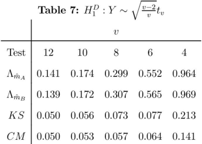
The first four alternatives attempt to classify alternatives in terms of departures in successive moments, the mean, variance skewness and kurtosis, while holding other moments constant. Notice though that the excess kurtosis of the standardised Chi-Square is in fact12/v.Thefinal experiment considers alternatives which are bi-modal. For alternatives A, B and D, the null hypothesis is satisfied for µ = 0, while for

alternatives C andD is obtained in the limit as v_{→ ∞}.

The simulated powers, based upon Monte Carlo critical values at the 5% sig-nificance level, of the likelihood ratio tests ΛmˆA and ΛmˆB and of the KS and CM

statistics are presented in Tables 3 through 8 in the Appendix. Collectively the pow-ers of the two likelihood ratio information criteria based tests are similar. Likewise the KS and CM have similar power properties to each other. For alternative A,

differing means, in fact the established tests have a slight power advantage. However for all other moment departures the ΛmˆA and ΛmˆB tests enjoy a significant power

advantage. In fact, in many cases, the power is several orders of magnitude higher. The same is true for the bi-modal alternatives.

As with the one-sample versions of the Kolmogorov-Smirnov and Cramér-von Mises tests, it would be possible, in principle, to utilise weighting functions, other than the unit, such as the particular case in Anderson and Darling (1952). For example, we might expect that tests with weight specifically in one tail or the other should fair better against skewed alternatives.

However, before concluding that it must therefore be possible to find versions of the established tests with powers comparable with those proposed here several limitations must be considered. Such tests are not yet really feasible, although Canner (1975) has some limited numerical evidence for a particularly weighted version of the Kolmogorov-Smirnov. Their asymptotic distributions will be nonstandard, and moreover as in Anderson and Darling (1952) will have to be developed on a case-by-case basis. Even then, as Marsh (2005)finds in the single sample goodness offit case, a particular weighting function might deliver high power against certain alternatives, but only at the expense of power against other alternatives. Consequently, in the absence of explicit knowledge of the direction, at least, of the alternative it would be difficult to justify any particular weighted version of either the Kolmogorov-Smirnov and Cramér-von Mises tests.

can be parameterised in terms of an infinite exponential family. Save for the use of the density estimator the test is essentially the Portnoy (1988) test applied to the problem of testing the simple hypothesisH0∗ :θ0x =θ0y. Although no nonparametric

test, in this setting, can claim optimality, at least in the asymptotic regimem, n_{→ ∞}, m3_/n

→0the proposed test will be coincident with a point optimal test for H∗.

0 .

4

Conclusions

This paper has proposed nonparametric two-sample tests based upon the criteria of Portnoy (1988), exploiting the series density estimator of rain (1974) and Barron and Sheu (1991). The asymptotic distribution of the test is standard under the null and diverges under the alternative, ensuring consistency. Numerical evidence suggests the finite sample performance of asymptotic critical values for the test is at least equivalent to those for the Kolmogorov-Smirnov test, slightly worse than those for the Cramér—von Mises tests. On the other hand evidence is presented which indicates a clear power superiority for the tests proposed in this paper.

References

Akaike, H. 1974. A new look at the statistical model identification. System identifi -cation and time-series analysis. IEEE Trans. Automatic Control AC-19, 716—723 Anderson, T.W. 1962. On the distribution of the two-sample Cramér-von Mises criterion. Annals of Mathematical Statistics, 33, 1148-1159.

Anderson, T.W. and D.A. Darling 1952. Asymptotic theory of certain ‘goodness-of-fit’ criteria based on stochastic processes. Annals of Mathematical Statistics, 23, 193-212.

Barron, A.R. and C-H. Sheu 1991. Approximation of density functions by sequences of exponential families. Annals of Statistics, 19, 1347-1369.

Burr, E.J. 1964. Small-sample distributions of the two-sample Cramér-von Mises’

W2 _{and Watson’sU}2_{. Annals of Mathematical Statistics, 35, 1091—1098.}

Canner, P.L. 1975. A simulation study of one- and two-sample Kolmogorov-Smirnov Statistics with a particular weight function. Journal of the American Statistical Association, 70, 209-211.

Chow, Y.S. and H. Teicher 1988. Probability theory, 2nd _{ed., Springer-Verlag, New}

York.

Claeskens, G. and N.L. Hjort 2004. Goodness of fit via nonparametric likelihood ratios. Skandanavian Journal of Statistics, 31, 487-513.

Crain, B.R. 1974. Estimation of distributions using orthogonal expansions. Annals of Statistics, 2, 454—463.

Crain, B.R. 1976. More on estimation of distributions using orthogonal expansions. Journal of the American Statistical Association, 71, 741—745.

Crain, B.R. 1977. An information theoretic approach to approximating a probability distribution. SIAM Journal of Applied Mathematics, 32, 339—346.

Conover, W.J. 1999. Practical Nonparametric Statistics, John Wiley and Sons, New York.

Darling, D.A. 1957. The Kolmogorov-Smirnov, Cramér-von Mises tests. Annals of Mathematical Statistics, 28, 223-238.

Dufour, J-M. and A. Farhat 2002. Exact nonparametric two-sample homogeneity tests. Goodness-of-fit tests and model validity (Paris, 2000), Statistics for Industry and Technology, Birkhäuser Boston, 435—448.

Kiefer, J. 1959. K-sample analogues of the Kolmogorov-Smirnov and Cramér-v. Mises tests. Annals of Mathematical Statistics, 30, 420-447.

Kim, P.J. 1969. On the exact and approximate sampling distribution of the two-sample Kolmogorov-Smirnov criterionDmn, m≤n. Journal of the American

Statis-tical Association, 64, 1625—1637.

05/24, University of York.

Portnoy, S. 1988. Asymptotic behaviour of likelihood methods for exponential families when the number of parameters tends to infinity. Annals of Statistics, 16, 356-366. Schwarz, G. 1978. Estimating the dimension of a model. Annals of Statistics, 6, 461-464.

Appendix

Proof of Theorem 1.

Proof. For part (i) we shall consider the likelihood ratios based on the two samples separately. Define x¯ = _n1

X

PnX

i=1φxi, where φxi = (φ1(xi), ..,φm(xi))0, and so for the

sample on X we have the series density estimator

pˆ_θx(x) = exp n nX ³ ˆ θ_x0x¯₋ψm ³ ˆ θx ´´o ,

where θˆx is the solution to the first line in (3). On basis of this estimated density we

can define the (log-)likelihood ratio by,

Λx_θˆ x,θˆy = ln à p_θˆ_x(x) p_θˆ_y(x) ! =nX n (ˆθx−θˆy)0x¯− ³ ψm(ˆθx)−ψm(ˆθy) ´o ,

where θˆy now solves the second line in (3). The expansions given in equations

(2.1)-(2.3) of Portnoy (1988) hold for any two values in_Rm, and so we can write

ψ0m ³ ˆ θx ´ =ψm0 ³ ˆ θy ´ + (ˆθx−θˆy)0ψ 00 m ³ ˆ θy ´ +1 2Eθˆy ·³ (ˆθx−θˆy)0Ux ´2 Ux ¸ +Λ(˜θ), (15)

where Λ(.) is a remainder and θ˜ lies on a line segment joining θˆx and θˆy and Ux =

Vx−E_θˆ_y[Vx], Vx ∼ph

³

ˆ

θy

´

andVx is distributed independently of X.

Since Λx_θˆ

x,θˆy is a likelihood ratio it is invariant to reparametrisations of the form θ → α +βθ, which will be exploited here. Moreover, p_θˆ_x(x) is in the exponential

family and hence so is p_θˆ_x(a+bx), consequently and without loss of generality we

can assume that x¯ is standardised in that

ψ_m0 ³θˆy

´

= 0 and ψ00_m³θˆy

´

=Im. (16)

Therefore, and since by definition ψ0

m ³ ˆ θx ´ = ¯x we can rewrite (15) as (ˆθx−θˆy) = ¯x− 1 2Eθˆy ·³ (ˆθx−θˆy)0Ux ´2 Ux ¸ +Λ(˜θ). (17) Multiplying (17) first by x¯0 we have (ˆθx−θˆy)0(ˆθx−θˆy) = (ˆθx−θˆy)0x¯− 1 2Eθˆy ·³ (ˆθx−θˆy)0Ux ´3¸ + (ˆθx−θˆy)0Λ(˜θ) (18)

while instead multiplying (17) by(ˆθx−θˆy)0 we get

(ˆθx−θˆy)0x¯= ¯x0x¯− 1 2Eθˆy ·³ (ˆθx−θˆy)0Ux ´2 (¯x0Ux) ¸ + ¯x0Λ(˜θ). (19)

Thus subtracting (19) from (18) yields

|(ˆθx−θˆy)0−x¯| = 1 2Eθˆy ·³ (ˆθx−θˆy)0Ux ´2³ ¯ x₋(ˆθx−θˆy) ´0 Ux ¸ +³(ˆθx−θˆy)−x¯ ´0 Λ(˜θ).

Noting that from (5) underH∗

0 we have|θˆx−θˆy|=Op

³p

m/nX

´

and moreover since the elements of Ux are bounded the moment condition required for Theorem 3.1 of

Portnoy (1988) are automatically satisfied, then as there it is true that ³ (ˆθx−θˆy)−x¯ ´0 Λ(˜θ) = Op õ m nX ¶2! . (20)

Using the inequality ¯ ¯ ¯ ¯E_θˆ_y ·³ ¯ x₋(ˆθx−θˆy) ´0 Ux ³ (ˆθx−θˆy)0Ux ´2¸¯¯ ¯ ¯ ≤ E_θˆ_y "µ³ ¯ x₋(ˆθx−θˆy) ´0 Ux ¶2#1/2 E_θˆ_y ·³ (ˆθx−θˆy)0Ux ´4¸1/2 , we then find, ¯ ¯ ¯ ¯1₂E_θˆ_y ·³ (ˆθx−θˆy)0Ux ´2³ ¯ x₋(ˆθx−θˆy) ´0 Ux ¸¯¯_¯ ¯=Op õ m nX ¶2! ,

similar to equation (3.7) of Portnoy (1988), although it should be noted that this applies for our standardising coordinates implying (16).

If instead we substitute (19) into (18) rather than subtracting then on account of (20) we also obtain |(ˆθx−θˆy)0(ˆθx−θˆy)−x¯0x¯|=Op õ m nX ¶2! .

Again noting (16) the likelihood ratio permits a Taylor expansion with remainder of the form, 2Λx_θˆ x,θˆy = 2 n ln¡p_θˆ_x(x) ¢ −ln³p_θˆ_y(x) ´o = nX ( (ˆθx−θˆy)0(ˆθx−θˆy) + 1 3Eθ∗ "µ³ ˆ θx−θˆy ´0 Ux∗ ¶3#) , whereθ∗ _∈³_θˆ x,θˆy ´

andUx∗ =Vx∗−Eθ∗[Vx∗],while also noting that again sinceUx∗ is a bounded random variable, then

Eθ∗ "µ³ ˆ θx−θˆy ´0 Ux∗ ¶3# =Op ³ |θˆx−θˆy|3 ´ =Op õ m nX ¶3/2! , and so 2Λx_ˆ θx,θˆy =nXx¯ 0_x¯+O p Ãs m3 nX ! . Since 2Λx_ˆ θx,θˆy −m √ 2m = nXx¯0x¯−m √ 2m +Op Ãs m2 nX ! ,

and given the martingale central limit theorem, for example Theorem 9.3.1 of Chow and Teicher (1988), which implies that

nXx¯0x¯−m

√

2m →dN(0,1),

so that noting m2/nX →0 then

2Λx_ˆ

θx,θˆy −m

√

To complete part (i) consider the sample _{yi}ni=1 derived form Y, then proceeding

exactly as above, for

Λy_θˆ x,θˆy =nY n (ˆθy−θˆx)0y¯− ³ ψm(ˆθy)−ψm(ˆθx) ´o ,

we can reparameterise according to θ_→γ =a+bθ, so that now

ψ0_m(ˆγx) = 0 and ψ 00

m(ˆγx) =Im.

Proceeding exactly as above and noting the invariance of the likelihood ratio we will have, 2Λy_ˆ θx,θˆy−m √ 2m = nXx¯0x¯−m √ 2m +Op Ãs m2 nY ! ∼N(0,1) +op(1).

Then since X andY are independent, adding the likelihood ratios gives

λ= 2³Λx_θˆ x,θˆy+Λ y ˆ θx,θˆy ´ −2m √ 2m →d N(0,2) +op(1),

which proves part (i).

For part (ii) put θ0x = θ0 6= θ0y under H1. Though θˆx and θˆy still exist and are

unique, now _|θˆx −θ0| and |θˆy −θ0| are Op(m). The uniqueness of θ0x and θ0y and

convexity of the exponential density imply that

θ0y 6=θ0x ⇒ψm(θ0x)6=ψm(θ0y),

and hence

nX(ψm(θ0x)−ψm(θ0y)) = O(nX).

Further, since thex0

isand hence theφk(xi)0s are i.i.d. with mean zero, the individual

elements of √nXx¯ satisfy 1 √_n X Ã_nX X i=1 φk(xi) ! =Op(1),

which follows from a standard central limit theorem. Differentiability of ψm(.) over

Rm _{ensures that underH}

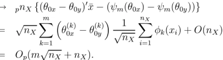
1 2Λx_θˆ x,θˆy = nX n (ˆθx−θˆy)0x¯− ³ ψm(ˆθx)−ψm(ˆθy) ´o

→ pnX{(θ0x−θ0y)0x¯−(ψm(θ0x)−ψm(θ0y))} = √nX m X k=1 ³ θ₀(k_x)₋θ₀(k_y)´_√1 nX nX X i=1 φk(xi) +O(nX) = Op(m√nX+nX).

Finally, since by assumptionm3_/n

X →0, then

2Λx_θˆ

x,θˆy =Op(nX),

and by an identical argument also 2Λy_ˆ

θy,θˆx = Op(nY), which is sufficient for

consis-tency under H1.

Tables 1-3: Monte Carlo rejection probabilities of the asymptotic critical values.

Table 1: H0 :X ∼Y ∼N(0,1)

sample size

Test sig. level 50 100 200 400

ΛmˆA 0.10 0.126 0.124 0.118 0.108 0.05 0.087 0.078 0.070 0.060 ΛmˆB 0.10 0.128 0.123 0.117 0.107 0.05 0.081 0.077 0.072 0.058 KS 0.10 0.068 0.073 0.077 0.087 0.05 0.033 0.036 0.039 0.042 CM 0.10 0.110 0.108 0.105 0.104 0.05 0.056 0.055 0.055 0.053

Table 2: H0 :X ∼Y ∼Exp(1)

sample size

Test sig. level 50 100 200 400

ΛmˆA 0.10 0.133 0.125 0.118 0.110 0.05 0.088 0.075 0.068 0.057 ΛmˆB 0.10 0.131 0.123 0.116 0.105 0.05 0.083 0.072 0.060 0.055 KS 0.10 0.065 0.069 0.077 0.087 0.05 0.033 0.035 0.038 0.041 CM 0.10 0.115 0.110 0.107 0.105 0.05 0.058 0.055 0.054 0.054 Table 3: H0 :X ∼Y ∼    N(₋1,1) with probability 0.5 N(1,1) with probability 0.5 sample size

Test sig. level 50 100 200 400

ΛmˆA 0.10 0.123 0.120 0.114 0.111 .05 0.084 0.075 0.064 0.059 ΛmˆB 0.10 0.123 0.113 0.111 0.108 0.05 0.081 0.066 0.063 0.053 KS 0.10 0.069 0.082 0.086 0.083 0.05 0.036 0.038 0.040 0.043 CM 0.10 0.114 0.110 0.108 0.106 0.05 0.058 0.055 0.054 0.054

Tables 4-8: Monte Carlo rejection probabilities under the alternative hypotheses. Table 4: HA 1 :Y ∼N(µ,1) µ Test 0.1 0.2 0.3 0.4 0.5 ΛmˆA 0.125 0.357 0.670 0.919 0.986 ΛmˆB 0.119 0.329 0.643 0.897 0.981 KS 0.137 0.410 0.718 0.922 0.991 CM 0.149 0.442 0.771 0.945 0.996 Table 5: H1B :Y ∼N(0,(1 +µ)2) µ Test 0.1 0.2 0.3 0.4 0.5 ΛmˆA 0.160 0.482 0.806 0.938 0.992 ΛmˆB 0.163 0.477 0.799 0.932 0.988 KS 0.066 0.139 0.274 0.413 0.624 CM 0.053 0.096 0.231 0.465 0.708 Table 6: HC 1 :Y ∼ χ2_(v)−v √ 2v v Test 35 30 25 20 15 10 5 ΛmˆA 0.192 0.209 0.251 0.295 0.393 0.619 0.928 ΛmˆB 0.171 0.198 0.234 0.274 0.394 0.620 0.922 KS 0.077 0.098 0.103 0.117 0.151 0.204 0.373 CM 0.075 0.083 0.094 0.113 0.133 0.175 0.349

Table 7: HD 1 :Y ∼ q v−2 v tv v Test 12 10 8 6 4 ΛmˆA 0.141 0.174 0.299 0.552 0.964 ΛmˆB 0.139 0.172 0.307 0.565 0.969 KS 0.050 0.056 0.073 0.077 0.213 CM 0.050 0.053 0.057 0.064 0.141 Table 8: HE 1 :Y ∼    N(₋µ,1) with probability0.5 N(µ,1) with probability0.5 µ Test .1 .3 .5 .7 .9 ΛmˆA 0.055 0.124 0.426 0.846 0.994 ΛmˆB 0.062 0.130 0.419 0.853 0.996 KS 0.050 0.068 0.117 0.321 0.740 CM 0.050 0.055 0.076 0.182 0.542