Utilizing Computer Vision and Data Mining for Predicting
Road Traffic Congestion
Mohsen Amoei
A Thesis in
The Concordia Institute for
Information Systems Engineering
Presented in Partial Fulfillment of the Requirements For the Degree of
Master of Applied Science (Quality Systems Engineering) at Concordia University
Montréal, Québec, Canada
March 2020
c
C
ONCORDIA
U
NIVERSITY
School of Graduate Studies
This is to certify that the thesis prepared By: Mohsen Amoei
Entitled: Utilizing Computer Vision and Data Mining for Predicting Road Traffic Congestion
and submitted in partial fulfillment of the requirements for the degree of Master of Applied Science (Quality Systems Engineering)
complies with the regulations of this University and meets the accepted standards with re-spect to originality and quality.
Signed by the final examining committee:
Dr. Chun Wang Chair Dr. Ciprian Alecsandru External Dr. Farnoosh Naderkhani Examiner Dr. Anjali Awasthi Thesis Supervisor Approved by
Dr. Mohammad Mannan, Graduate Program Director
March 18, 2020
Dr. Amir Asif, Dean
Abstract
Utilizing Computer Vision and Data Mining for Predicting Road Traffic
Congestion
Mohsen Amoei
Traffic Congestion wastes time and energy, which are the two most valuable commodi-ties of the current century. It happens when too many vehicles try to use a transportation infrastructure without having enough capacity. However, researches indicate that adding extra lane without studying the future consequences does not improve the situation. Our goal is to add another layer of information to the traffic data, find which type of vehicles are contributing to road traffic congestion, and predict future road traffic congestion and demands based on the historical data.
We collected more than 400,000 images from traffic cameras installed in Autoroute 40, in the city of Montreal. The images were collected for five consecutive weeks from different locations from April 14, 2019, up until May 18, 2019. To process these images and extract useful information out of them, we created an object detection and classification model using the Faster RCNN algorithm. Our goal was to be able to detect different types of vehicles and see if we have traffic congestion in an image. In order to improve the accuracy and reduce the error rate, we provided multiple examples with different conditions to the model. By introducing blurry, rainy, and low light images to the model, we managed to build a robust model that could do the detection and classification task with excellent accuracy.
Furthermore, by extracting the information from the collected images, we created a dataset of the number of vehicles in each location. After analyzing and visualizing the data, we find out the most congested areas, the behavior of the traffic flow during the day, peak hours, the contribution of each type of vehicle to the traffic, seasonality of the data, and where we can see each type of vehicle the most.
Finally, we managed to predict the total number of congestion incidents for seven days based on historical data. Besides, we were able to predict the total number of different types of vehicles on the road as well. In order to do this task, we developed multiple Regression,
Deep Learning, and Time Series Forecasting models and trained them with our vehicle count dataset. Based on the experimental results, we were able to get the best predictions with the Deep Learning models and succeeded in predicting future road traffic congestion with excellent accuracy.
Keywords: Computer Vision, Data Mining, Time Series Forecasting, Road Traffic Congestion, Deep Learning
Acknowledgments
First and foremost, I would like to express my sincere gratitude to my advisor, Professor Anjali Awasthi, for her constant support throughout my journey at Concordia University.
I would also like to thank my fellow labmates, for their support. Taiwo, Hassan, Negar, Suganya, Ujjwal, Akhil, and Safwan. It was fun being your labmate.
I would like to thank my colleagues at SAP company for helping me and sharing their knowledge with me. Benjamin, Marc-Andre, Andre, Urmil, Sabrina, Tarandeep, Bianca, Nitheesh and Ishrar, I’m lucky to have the chance to work alongside you all.
I want to thank my friends for always being there and helping me coping with hard times. Ramtin, Parsa, and Adam, thanks for all the good times.
I must thank my dear Behshid for her unconditional and unparalleled love and support. It would be impossible to do it without you.
I must express my profound gratitude to my parents and my dear sister, Mehrnaz, for providing me with unfailing support and continuous encouragement throughout my years of study and through the process of researching and writing this thesis. This accomplishment would not have been possible without them. Thank you.
Contents
List of Figures ix
List of Tables xiv
1 Introduction 1 1.1 Research Objective . . . 2 1.2 Contributions . . . 3 1.3 Thesis Structure . . . 4 2 Background 5 2.1 Introduction . . . 5
2.2 Road Traffic Congestion . . . 5
2.3 Deep Learning Platforms and Libraries . . . 6
2.4 Performance Metrics . . . 10
2.4.1 Estimation and Prediction Performance Metrics . . . 10
2.5 Object Detection and Classification Algorithms . . . 12
2.5.1 Convolutional Neural Networks (CNN) . . . 12
2.5.2 Region-Based Convolutional Neural Networks (R-CNN) . . . 13
2.6 Time Series Forecasting Algorithms and Models . . . 16
2.6.1 Regression Analysis . . . 17
2.6.3 Time series Forecasting Models . . . 22
2.7 Conclusion . . . 25
3 Literature Review 26 3.1 Introduction . . . 26
3.2 Object Detection and Classification . . . 27
3.2.1 Application Focused Researches . . . 27
3.2.2 Model Improvement Oriented Researches . . . 28
3.3 Time Series Forecasting . . . 29
3.3.1 Road Traffic Prediction Related Researches . . . 29
3.3.2 Non Road Traffic Prediction Related Researches . . . 30
3.4 Conclusion . . . 31
4 Methodology 32 4.1 Introduction . . . 32
4.2 High-level Model Description . . . 32
4.3 Data Acquisition . . . 34
4.3.1 Data Collection . . . 34
4.4 Object Detection and Classification . . . 37
4.4.1 Data Preparation . . . 37
4.4.2 Supervised pre-training . . . 40
4.4.3 Faster R-CNN Model . . . 41
4.5 Time Series Traffic Forecasting . . . 44
4.5.1 Data Preparation . . . 44
4.5.2 Regression Analysis . . . 45
4.5.3 Deep Learning Methods . . . 47
4.6 Conclusion . . . 53
5 Experimental Results 54 5.1 Introduction . . . 54
5.2 Object Detection and Classification Models . . . 54
5.2.1 Data Cleaning Image Classification Model . . . 55
5.2.2 Vehicle Detection and Classification Model . . . 57
5.3 Data Visualization . . . 71
5.4 Time Series Forecasting . . . 80
5.4.1 Regression Analysis Models . . . 80
5.4.2 Deep Learning Models . . . 96
5.4.3 Time Series Forecasting Models . . . 107
5.5 Conclusion . . . 118
6 Conclusion and Future Works 120 6.1 Conclusion . . . 120
6.2 Future Works . . . 122
List of Figures
1 Traffic status of the city of Montreal on 18:36 February 25th, 2020. Cour-tesy of (TomTom, 2019) . . . 7 2 LabelImg Platform Environment . . . 9 3 Object detection system overview for R-CNN, Courtesy of (Girshick et al.,
2014) . . . 13 4 Fast R-CNN architecture, Courtesy of (Girshick, 2015) . . . 15 5 Region Proposal Network (RPN) architecture, Courtesy of (Ren et al., 2015) 16 6 Model of an Artificial Neuron. Courtesy of (Agatonovic-Kustrin and
Beres-ford, 2000) . . . 20 7 Model of an Artificial Neural Network. Courtesy of (Anderson and
Mc-Neill, 1992) . . . 20 8 On the left side we can see a typical RNN and on the right side is the
unfolding version. Courtesy of (Tai and Liu, 2016). . . 21 9 LSTM Memory Cell with Gates. Courtesy of (Soutner and Müller, 2013). . 22 10 Analyst in the loop model. Courtesy of (Taylor and Letham, 2018) . . . 24 11 The Methodology Steps. From left to Right: (1) Getting Data from Traffic
Cameras, (2) Using Computer Vision to Extract Information, (3) Creat-ing the Historical Dataset of the Vehicle and Congestion Count, (4) De-velop Several Time Series Forecasting Models, (5) Visualize the Predic-tions, Compare the Results and Find the Best Model . . . 33
12 Traffic cameras provided by Quebec511 in city of Montreal. Courtesy of (Google-Maps, 2019)(Quebec511, 2019) . . . 35 13 Auto route 40. Courtesy of (Google-Maps, 2019) . . . 36 14 Images Collected from Traffic Cameras. Courtesy of (Quebec511, 2019) . . 36 15 Traffic Camera Footage is Unavailable(No-Footage). Courtesy of
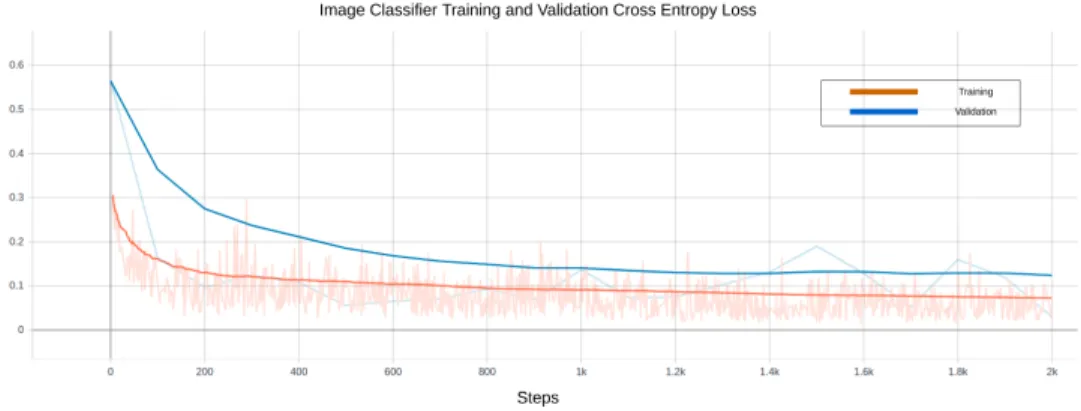
(Que-bec511, 2019) . . . 38 16 An Example of an Image with All the Object Marked in it Using LabelImg 40 17 CNN Time Series Forecasting Model Architecture Flowchart . . . 49 18 LSTM Time Series Forecasting Model Architecture Flowchart . . . 51 19 Cross Entropy Loss of the Inception v3 Data Cleaning Image Classification
Model . . . 55 20 Accuracy of the Inception v3 Data Cleaning Image Classification Model . . 56 21 Classification(Objectness) Loss Of the Faster RCNN Model . . . 59 22 Localization(Detection) Loss Of the Faster RCNN Model . . . 60 23 The Sum of the Classification and Localization Loss(Total Loss) . . . 60 24 An Example of the Object Detection Model Output on Images with Normal
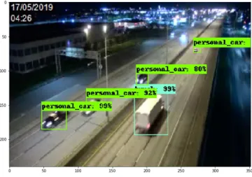
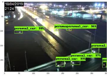
Day Light Setting . . . 61 25 An Example of the Object Detection Model Output on Images with Normal
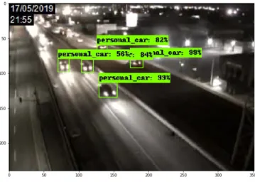
Night Light Setting . . . 62 26 An Example of the Object Detection Model Output on Images with Low
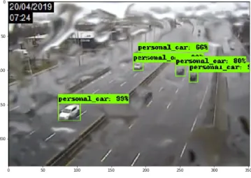
Light Setting . . . 63 27 An Example of the Object Detection Model Output on Images with Rain
Condition . . . 64 28 An Example of the Object Detection Model Output on Images with Low
29 An Example of the Object Detection Model Output on Images with
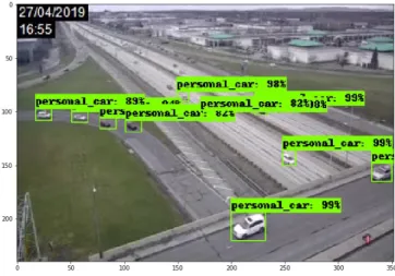
Com-plex Road Architecture . . . 65
30 An Example of the Object Detection Model Output on Images with Com-plex Road Architecture and Low Light Setting . . . 66
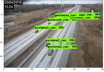
31 An Example of the Object Detection Model Output on Images with Per-sonal Cars In Them . . . 67
32 An Example of the Object Detection Model Output on Images with Trucks In Them . . . 67
33 An Example of the Object Detection Model Output on Images with Buses In Them . . . 68
34 An Example of the Object Detection Model Output on Images with Road Traffic Congestion In Them . . . 69
35 An Example of the Object Detection Model Output on Images with Lots of Vehicles in Them but No Traffic Congestion . . . 70
36 The Vehicle Count Dataset . . . 70
37 Total Number of Personal Car in each Hour of the Day . . . 71
38 Total Number of Trucks in each Hour of the Day . . . 72
39 Total Number of Buses in each Hour of the Day . . . 73
40 Total Number of Recorded congestion in each Hour of the Day . . . 74
41 Total Number of Personal Cars in each Location During the Month . . . 75
42 Total Number of Trucks in each Location During the Month . . . 76
43 Total Number of Buses in each Location During the Month . . . 77
44 Total Number of Congestion Recorded in each Location During the Month . 78 45 Heatmap of Correlation Between the Features . . . 79
46 Prediction Results for Number of Personal Cars with Linear Regression Model . . . 81
47 Prediction Results for Number of Trucks with Linear Regression Model . . 82 48 Prediction Results for Number of Buses with Linear Regression Model . . . 83 49 Prediction Results for Number of Recorded congestion with Linear
Regres-sion Model . . . 85 50 Prediction Results for Total Number of Personal Car with Polynomial
Re-gression Model with Degree Three . . . 87 51 Prediction Results for Total Number of Trucks with Polynomial Regression
Model with Degree Two . . . 88 52 Prediction Results for Total Number of Bus with Polynomial Regression
Model with Degree Two . . . 89 53 Prediction Results for Total Number of Personal Car with Polynomial
Re-gression Model with Degree Two . . . 90 54 Prediction Results for Number of Personal Cars with Random Forest
Re-gression Model with 18 Estimator . . . 92 55 Prediction Results for Number of Trucks with Random Forest Regression
Model with One Estimator . . . 93 56 Prediction Results for Number of Buses with Random Forest Regression
Model with Four Estimator . . . 94 57 Prediction Results for Traffic Congestion with Random Forest Regression
Model with Five Estimator . . . 95 58 Prediction Results for Total Number of Personal Car with CNN Model 2 . . 98 59 Prediction Results for Total Number of Trucks with CNN Model 3 . . . 99 60 Prediction Results for Total Number of Buses with CNN Model 3 . . . 101 61 Prediction Results for Total Number of Road Traffic Congestion with CNN
Model 1 . . . 102 62 Prediction Results for Total Number of Personal Cars with LSTM Model 1 104
63 Prediction Results for Total Number of Trucks with LSTM Model 2 . . . . 105 64 Prediction Results for Total Number of Buses with LSTM Model 4 . . . 106 65 Prediction Results for Total Number of Road Traffic Congestion with LSTM
Model 3 . . . 108 66 Prediction Results for Total Number of Personal Cars with ARIMA Model . 109 67 Prediction Results for Total Number of Trucks with ARIMA Model . . . . 111 68 Prediction Results for Total Number of Buses with ARIMA Model . . . 112 69 Prediction Results for Total Number of Road Traffic Congestion with ARIMA
Model . . . 113 70 Prediction Results for Total Number of Personal Cars with Prophet Model . 114 71 Prediction Results for Total Number of Trucks with Prophet Model . . . 115 72 Prediction Results for Total Number of Buses with Prophet Model . . . 117 73 Prediction Results for Total Number of Road Traffic Congestion with Prophet
List of Tables
1 Collected Information from Quebec 511 website . . . 37
2 Table of all the footages we expect from traffic cameras . . . 39
3 Weather Situation in City of Montreal During the Year (NOAA, 2019). . . 41
4 Convolutional Neural Network Model Architectures for Time Series Fore-casting Models . . . 49
5 Long Short Term Memory Time Series Forecasting Models . . . 50
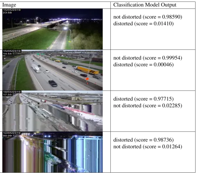
6 Table of the Results of the Data Cleaning Image Classification Model on Different Images . . . 57
7 Faster RCNN Model Hyper-Parameters . . . 58
8 Momentum Optimizer Hyper-Parameters . . . 58
9 Faster RCNN Model Loss Function Hyper-Parameters . . . 58
10 Prediction Results and the Performance Metrics of the Linear Regression Model on Total Number of the Personal Car . . . 81
11 Prediction Results and the Performance Metrics of the Linear Regression Model on Total Number of the Trucks . . . 83
12 Prediction Results and the Performance Metrics of the Linear Regression Model on Total Number of the Buses . . . 84
13 Prediction Results and the Performance Metrics of the Linear Regression Model on Total Number of Road Traffic Congestion . . . 85
14 Prediction Results and the Performance Metrics of the Polynomial Regres-sion Model on Total Number of Personal Car . . . 86 15 Prediction Results and the Performance Metrics of the Polynomial
Regres-sion Model on Total Number of Trucks . . . 88 16 Prediction Results and the Performance Metrics of the Polynomial
Regres-sion Model on Total Number of the Buses . . . 89 17 Prediction Results and the Performance Metrics of the Polynomial
Regres-sion Model on Total Number of Road Congestion . . . 90 18 Prediction Results and the Performance Metrics of the Random Forest
Re-gression Model on Total Number Personal Cars . . . 91 19 Prediction Results and the Performance Metrics of the Random Forest
Re-gression Model on Total Number of Trucks . . . 93 20 Prediction Results and the Performance Metrics of the Random Forest
Re-gression Model on Total Number of Buses . . . 95 21 Prediction Results and the Performance Metrics of the Random Forest
Re-gression Model on Total Number of Road Traffic Congestion . . . 96 22 Convolutional Neural Network Time Series Forecasting Models . . . 97 23 Convolutional Neural Network Time Series Forecasting Models Results
with Performance Metrics for Personal Cars . . . 98 24 Convolutional Neural Network Time Series Forecasting Models Results
with Performance Metrics for Trucks . . . 99 25 Convolutional Neural Network Time Series Forecasting Models Results
with Performance Metrics for Buses . . . 100 26 Convolutional Neural Network Time Series Forecasting Models Results
with Performance Metrics for Road Traffic Congestion . . . 101 27 Long Short Term Memory Time Series Forecasting Models . . . 103
28 Long Short Term Memory Time Series Forecasting Models Results and Performance Metrics for Total Number of Personal Cars . . . 103 29 Long Short Term Memory Time Series Forecasting Models Results and
Performance Metrics for Total Number of Trucks . . . 105 30 Long Short Term Memory Time Series Forecasting Models Results and
Performance Metrics for Total Number of Buses . . . 106 31 Long Short Term Memory Time Series Forecasting Models Results and
Performance Metrics for Total Number of Road Traffic Congestion . . . 107 32 ARIMA Model Results and Performance Metrics for Total Number of
Per-sonal Cars . . . 109 33 ARIMA Model Results and Performance Metrics for Total Number of Trucks110 34 ARIMA Model Results and Performance Metrics for Total Number of Buses 111 35 ARIMA Model Results and Performance Metrics for Total Number of Road
Traffic Congestion . . . 113 36 Prophet Model Results and Performance Metrics for Total Number of
Per-sonal Cars . . . 114 37 Prophet Model Results and Performance Metrics for Total Number of Trucks115 38 Prophet Model Results and Performance Metrics for Total Number of Buses 116 39 Prophet Model Results and Performance Metrics for Total Number of Road
Chapter 1
Introduction
"The two most valuable commodities of the 21st century are time and energy; traffic con-gestion wastes both" (Pan et al., 2012). Traffic is one of the most critical problems of major cities like Montreal. Our goal is to add another layer of information to the traffic data, find which type of vehicles are contributing to road traffic congestion, and predict future road traffic congestion and demands based on the historical data.
We collected more than 400,000 images from traffic cameras installed in Autoroute 40, in the city of Montreal. The images were collected for five consecutive weeks from different locations from April 14, 2019, up until May 18, 2019. To process these images and extract useful information out of them, we created an object detection and classification model using the Faster RCNN algorithm. Our goal was to be able to detect different types of vehicles and see if we have traffic congestion in an image. In order to improve the accuracy and reduce the error rate, we provided multiple examples with different conditions to the model. By introducing blurry, rainy, and low light images to the model, we managed to build a robust model that could do the detection and classification task with excellent accuracy.
Furthermore, by extracting the information from the collected images, we created a dataset of the number of vehicles in each location. After analyzing and visualizing the
data, we find out the most congested areas, the behavior of the traffic flow during the day, peak hours, the contribution of each type of vehicle to the traffic, seasonality of the data, and where we can see each type of vehicle the most.
Finally, we managed to predict the total number of congestion incidents for seven days based on historical data. Besides, we were able to predict the total number of different types of vehicles on the road as well. In order to do this task, we developed multiple Regression, Deep Learning, and Time Series Forecasting models and trained them with our vehicle count dataset. Based on the experimental results, we were able to get the best predictions with the Deep Learning models and succeeded in predicting future road traffic congestion with excellent accuracy.
1.1
Research Objective
We are all familiar with traffic congestion and experience it in our daily commutes. Traffic congestion happens when too many vehicles try to use a transportation infrastructure with-out having enough capacity (Papageorgiou et al., 2003). However, researches indicate that adding extra lane without studying the future consequences does not improve the situation (Duranton and Turner, 2011).
In order to study the data in a more granular fashion, we decided to process the image data instead of sensor or GPS collected data. By using the image dataset, we will have all the data we need, but we have to find a way to extract information and use them in our favor. In this research, without installing new equipment, we managed to create a valuable image dataset and used state-of-the-art algorithms to convert the data into information.
By adding another layer of information to the traffic data, we will be able to understand the contribution of each type of vehicle to the traffic, analyze the demand, and the behavior of traffic flow in more detail and predict future events with more accuracy. This way, we can prioritize the locations which need more infrastructure and find more insightful information
about the general distribution and the balance of the resources and the demand in the city of Montreal.
1.2
Contributions
The contributions of this research are divided into three main sections:
• Data Collection, Cleaning, and PreprocessingAs we mentioned in previous para-graphs, our goal in this thesis is to predict traffic congestion by using image datasets instead of GPS or sensor-generated data. In the first step, We built an image dataset from the Autoroute 40 in the city of Montreal traffic cameras. We collected more than 400,000 images for five consecutive weeks. After analyzing the data, we de-veloped an image classifier to clean the data and reduce the amount of noise in the image dataset. The main contribution of this step is a clean image dataset from the traffic cameras.
• Implementing Object detection and Classification Models The next step after building the image dataset is extracting information out of them. We trained an object detection and classification model using the Faster RCNN algorithm and managed to detect each type of vehicle and traffic congestion in an image. We applied this model to the entire image dataset and created a vehicle count dataset. After analyzing the data, we managed to find the contribution of each type of vehicle (personal car, bus, truck) to the traffic, traffic flow behavior, peak hours, and trends for each type of vehicle. The main contribution of this step alongside the mentioned results is a clean vehicle and congestion count dataset with a time series relationship.
• Developing Multiple Time Series Forecasting Models After creating the vehicle count dataset, we can use this dataset to predict future demand and traffic congestion.
In order to do this task, we developed multiple time series forecasting models with different Regression, Deep Learning, and time series forecasting algorithms. We researched to find the best model and how we can get the best prediction results with different architectures. The main contribution of this step is predicting future traffic congestion, the total number of each type of vehicle, and the best model to do this task.
1.3
Thesis Structure
In this thesis, first, we start with definitions about the algorithms and tools we are going to use for this research and get familiar with them. Moreover, we review the researches that are related to the work we are doing in this thesis. Later, we discuss our methodology and how we implement our models. After the methodology, we go over the results that we obtained from each approach and compare them. In the end, we discuss the overall results and the next steps for this research.
Chapter 2
Background
2.1
Introduction
In this section, we discuss the materials we need to develop this thesis. In our research in each step of the works, we use different platforms and different libraries, which we go over them and get familiarized with them. Furthermore, we explore the ways that we can utilize them in our favor to get the best results. First, we explore the deep learning platforms and libraries and discuss the advantages and disadvantages of each of them. Later, we explore the performance metrics and see how we can evaluate our models. After discussing performance metrics, we explore the object detection and classification algorithms and get to know more about their architecture and capabilities. In the end, we discuss the time series forecasting algorithms and explore some of the existing libraries for these kinds of tasks as well.
2.2
Road Traffic Congestion
We are all familiar with traffic congestion and experience it in our daily commutes. It wastes energy and time and has lots of negative effects on the environment. (Bharadwaj
et al., 2017) conducted a field study in order to find the relationship between fuel consump-tion and the greenhouse gas emission. The results of this study shows that the more travel time under road traffic congestion is significantly responsible for moreCO2emissions from
the fuel consumption. On the other hand it has negative impacts on the public heath as well. (Levy et al., 2010) evaluate the public health impacts of being exposed to fine particulate matter concentrations associated with traffic congestion. The analyses shows that the public health impact is significant enough and should be considered when evaluating new policies for alleviating the traffic situation.
Traffic congestion happens when too many vehicles try to use a transportation infras-tructure without having enough capacity (Papageorgiou et al., 2003). However, researches indicate that adding extra lane does not necessarily improve the situation. (Duranton and Turner, 2011) investigated the effect of lane kilometers of roads on vehicle-kilometers travel for different types of road in the US cities and provided direct evidence that the extension of most major roads resulted in a proportional increase in traffic.
Based on the TomTom Traffic indexing (TomTom, 2019) congestion level of the city of the Montreal is ranked third in the Canada, tenth in North America and 138th Globally. TomTom collects data from GPS devices based on the actual driven trips. In figure 1 we can see an screenshot of the TomTom website, informing the current traffic situation of the city of Montreal.
2.3
Deep Learning Platforms and Libraries
To create different models from simple Regression models to more complex deep neural network models, we need to use some external libraries and platforms. Our goal in this section is to explore our options and get familiar with the advantages and disadvantages of each one. Later, we see how we can utilize them in our research to get the best results.
Figure 1: Traffic status of the city of Montreal on 18:36 February 25th, 2020. Courtesy of (TomTom, 2019)
Tensorflow Or Tf in short, is an open-source platform for machine learning. It was de-veloped by Google and has a comprehensive stes of tools, which makes it one of the best libraries for machine learning studies. Tensorflow computations are exposed as data flow graphs and have a unique tool called Tensorboard, which plots all the necessary graphs dur-ing and after the traindur-ing phase. One of the disadvantages of Tensorflow is the complexity and difficulty of creating a simple model and deploying it. (Tensorflow, 2019).
Keras In the previous paragraph, we explained what is Tensorflow and for what purposes we can use it. We mentioned that one of the disadvantages of Tensorflow is the complexity of developing simple neural networks and create a model from them. Keras, which is a high-level neural network API, is the solution to this problem. It was written in Python programming language, and it is capable of running on top of the platforms like Tensor-flow.(Keras, 2019).
Keras has different libraries with predefined neural network models and algorithms. We can create a simple neural network by just calling the library and put them into the desired order and architecture. We use Keras mainly for training our deep learning models for time
series traffic forecasting.
Scikit-Learn Scikit-Learn or Sklearn is a free machine learning library developed for Python programming language and features many regression, classification, and clustering algorithms. We mainly use the Sklearn for our regression analysis task and evaluating our predictions with the performance metrics available in the library (Scikit-learn, 2019).
Numpy When we are dealing with data, most of the time, they are in the form of big matrices or arrays. On the other hand, most of the complicated calculations happen when we are dealing with a large amount of data, so we need a library not only to handle these calculations correctly but also do it in the shortest time possible. Numpy is a library written mostly in the C language and developed for different languages to carry out large-scale and multidimensional mathematical calculations. Most of the libraries dealing with large scale data or massive calculations use Numpy in the back-end. We use Numpy for a variety of tasks from getting mean or median to transform an image data to a three-dimensional array of values to process it (Numpy, 2019).
Pandas Python has a long history of being one of the best programming languages for data manipulation and preparation, but not for data analysis and modeling. Python Data Analysis Library or Pandas is an open-source library that provides high-performance data structures and data analysis tools for the Python programming language. As mentions in the previous paragraph, Pandas is one of the libraries that use Numpy for handling all the large-scale calculations and data manipulation. We mainly use Pandas for creating different data frames, data manipulations and performing data transformations (Pandas, 2019).
Matplotlib Data visualization can help us get better insights into our data. It is easier to understand the differences and catch the essential information in one glance. Matplotlib is one of the best libraries developed for python language for data visualization purposes.
It offers a variety of 2D and 3D plots with different shapes and lots of configurations. Creating plots and fugues alongside, providing different text information and changing the color map of the plots is not a hard task in Matplotlib. We use this library mainly for visualizing our datasets, creating images with bounding-boxes on them and plotting the predictions next to the target values for time series forecasting models (Matplotlib, 2019).
Seaborn Seaborn is a Python library which is built on top of Matplotlib to create more colorful plots. (Seaborn, 2019).
LabelImg Our image dataset consists of images with lots of information in them. It would be hard for the model to understand each type of vehicle on its own from these images. To help the model understand what exactly it should look for, we annotate each type of vehicle in the image and create another file with coordinates of the mentioned annotations in it. The new file is in the XML format and has the same name as the image. To do this task, we used a graphical annotation tool called LabelImg. LabelImg is written in Python programming language and uses the QT library for its graphical interface, which makes it easy for us to annotate all the images that we need for the training purposes. In Figure 2 you can see the environment of the LabelImg (Tzutalin, 2015).
2.4
Performance Metrics
Regardless of the model and its purpose, we are always curious to see how the model performs on the test dataset. Our goal in this section is to explore different performance metrics that we can use to evaluate our models. Since there are different performance metrics for different tasks, we separate them into two different subsections to explore them based on their architecture and their results. First, we explore how we can measure the performance of a classification task, and later we discuss different prediction performance metrics and how we utilize each of them.
2.4.1
Estimation and Prediction Performance Metrics
In the previous section, we discussed the performance metrics that can help us get a better understanding of the performance of our classification models. In this section, we explore the metrics that we can use to know the performance of our regression and time series forecasting models. We what are the advantages and disadvantages of each metrics and see how we can utilize them to understand our models better.
Mean Squared Error Mean Squared Error, which also called Mean Squared Deviation, is an estimator measure the average of the squares of the errors. The errors in our case are the distance between the target values and predicted values. Mean Squared error can be calculated as follows: M SE= 1 n n X i=1 (Yi−Yˆi)2 (1)
One thing that we can notice from (1) is that the distance between the target and the pre-dicted value is squared so that the total value can accumulate to a large value.
Mean Absolute Error Mean Absolute Error, like MSE, measures the distance between the target and predictions.
M AE = 1 n n X i=1 |Yi−Yˆi| (2)
R2 Score We explored two different ways to measure the distance between the target values and prediction values in previous paragraphs. One of the problems with the previous approaches is that since we are concerned with the distance of two values, we are not considering their scale into the equation. This means that for larger values, we have bigger errors, which does not necessarily represent the performance of the model. To solve this issue and get a better understanding of the model’s performance, we can use R squared, which is defined as follows:
SStot = n X
i=1
(yi−yˆi)2 (3)
(3) represents the total sum of the squares which is proportional to the variance of the data. SSres = X i (yi−fi)2 = X i e2i (4)
(4) is the sum of the squares of the residuals.
R2 = 1− SSres SStot
(5) (5) is one of the most general definitions of the R2 score or the coefficient of determi-nation. We can see the R2 score can be ranging from minus infinity to one. The bigger the value of R2 score is, the better the model can explain the behavior of the data, or in other words, The closer the R2 score value is to one, the more accurate the model is.
2.5
Object Detection and Classification Algorithms
In this section, we discuss object detection and classification methods that we can use to train our vehicle detection model. First, we explore the Convolutional Neural Network (CNN) and its advantages in detail. Later we discuss Faster Region-based Convolutional Neural Network (Faster R-CNN) and explore why we are building our model with this algorithm.
2.5.1
Convolutional Neural Networks (CNN)
CNN was inspired based on the research of Hubel and Wisel on the visual cortex of a cat (Hubel and Wiesel, 1962). They proposed two different complexity for the cell structure of neurons in the visual cortex of the cat. One activates when the cat sees a simple shape. The other one activates when the cat sees a shifted or rotated version of the original object. In 1998, Le Cunn, Bottou, Bengio, and Haffner in the handbook of brain theory and neural networks proposed CNNs (LeCun et al., 1995).
Although the idea of CNN is not new, it became popular relatively recently. The main reasons contributing to the recent usage of CNNs are(Koirala et al., 2018):
• The exponential growth in processing power • Data collection devices like cameras and sensors
In order to be able to utilize a CNN model and get good results, you need to have a huge amount of data and enough computational power to process it. The mentioned factors helped cover these problems.
Moreover, the publication of Krizhevsky’s article (Krizhevsky et al., 2012) showed a massive improvement for object detection and image recognition using ImageNet Deng et al. (2009) dataset, which drew a lot of attention from the researchers to the potential of CNN in the image recognition area (Yosinski et al., 2014).
In this thesis, we will discuss on the applications of CNN for object detection and classification task and time series forecasting task as well. Later in this chapter, we describe a specific type of the CNN family, R-CNN, and explain how this type, in particular, helps us develop a vehicle classifier.
2.5.2
Region-Based Convolutional Neural Networks (R-CNN)
We discussed how CNN became famous for its capabilities in image processing. In this section, we will discuss an approach that made a huge improvement in this area. Gir-shick (GirGir-shick et al., 2014) named the approach R-CNN: Regions with CNN features and the reason behind it was the fact that they combined region proposals with CNNs. In fig-ure 3, we can see the architectfig-ure of the RCNN in four steps. This approach combined two key insights:
1. Enables applying high-capacity CNN to bottom-up region proposals to localize and segment objects
2. In case of scarce labeled training data, supervised pre-training for auxiliary task fol-lowed by domain-specific fine-tuning yields a significant performance boost.
Figure 3: Object detection system overview for R-CNN, Courtesy of (Girshick et al., 2014)
The proposed object detection model consists of three modules. The objective of the first module is to generate category independent region proposals. These proposals are
regions that are fed to the next module as the areas that are most likely to find an object. The next module is a CNN that looks into each of the proposed regions to extract a fixed-length feature vector. The third module is a set of class-specific linear Support Vector Machines (SVMs). R-CNN also managed to achieve a mean average precision(mAP) of 53.7% on PASCAL VOS 2010. (Girshick et al., 2014) Although the accuracy of R-CNN is good, it has some major drawbacks, which makes it challenging to use. Some of these drawbacks are (Girshick, 2015):
1. Multi-stage pipeline for training the model
2. Training the model requires lots of space and time
3. Applying the model on images for object detection is slow
In the next paragraph we will explore a way to improve speed and accuracy of the R-CNN model.
Fast R-CNN In the previous paragraph, we discussed how R-CNN works and what are the advantages and disadvantages of this algorithm. One of the significant drawbacks of R-CNN is the speed for the training of using the model for object detection. The main reason that the R-CNN is slow is due to the fact that it operates a ConvNet forward pass for each of the object proposals without sharing the computations(Girshick, 2015). The goal of Fast R-CNN is to fix the mentioned problems with the R-CNN. In figure 5, we can see the architecture of the new approach. An input image and the multiple regions of interest are input into a fully convolutional neural network. There is a fixed-sized feature map for each region of interest (ROI). Each ROI is pooled into the mentioned feature map and then mapped into a feature vector by fully connected layers. For each ROI, there are two output vectors in the network:
• Per-class bounding box regression offsets.
Figure 4: Fast R-CNN architecture, Courtesy of (Girshick, 2015)
The advantages of Fast RCNN are (Girshick, 2015):
1. The Higher detection quality(mAP) than previous methods 2. Training is no longer a multi-stage and using a multi-task loss 3. Training can update all network layers
4. No disk storage is required for feature caching
Faster R-CNN In the previous paragraphs, we explored the state-of-art approaches for object detection and classification. First, we discussed the advantages and disadvantages of R-CNN and how Fast R-CNN answered those issues. In this paragraph, we explore another approach that tried to improve these models from both speed and accuracy perspective. The Faster R-CNN approach tries to reduce the training and testing time of the model by improving the region proposal computations. The new region proposal network (RPN) shares full-image convolutional features with the detection network resulting in cost-free region proposals(Ren et al., 2015). The architecture of the new RPN can be seen in the figure 5.
The results in terms of both speed and accuracy for the Faster R-CNN object detec-tion system was 73.2% mAP on PASCAL VOC 2007 and 70.4% mAP on PASCAL VOC
Figure 5: Region Proposal Network (RPN) architecture, Courtesy of (Ren et al., 2015)
2012(Ren et al., 2015). Since we have a limited amount of computational resources, we need a model to do the calculations fast while not sacrificing the accuracy, which with Faster R-CNN, we can achieve these goals.
2.6
Time Series Forecasting Algorithms and Models
In this section, we discuss different time series forecasting algorithms and explore the mathematical idea behind each of them. First, we talk about different regression analy-sis algorithms, explore their differences and similarities, and discuss the advantages and disadvantages of each of them based on their capabilities. Later, we explore different neu-ral network models and try to understand how each architecture of these networks work and what are the ways to find the fine-tuned models. In the end, we explore two different models that are mainly developed for different time series forecasting tasks and talk about how they work and what could be achieved using them.
2.6.1
Regression Analysis
There are many different types of regression available to study, but in this thesis, we mainly focused on three different regression analysis algorithms. First, we start with the simplest form of regression, which is Linear Regression, and then we explore the Polynomial Re-gression. At last, we see what Random Forest Regression is and how we can improve our predictions with it.
Linear Regression Linear regression is the simplest form of regression analysis, which studies the linear relationship between two variables. The linear regression equation (6) is a straight line that defines the effect of independent variableX on the dependent variable Y.
Y =aX+b (6)
In (6), a is the slope of the line, and b is they-intersect. The regression line lets one to predict the value of dependent variable Y from the independent variableX (Schneider et al., 2010). To mention a few examples, we would be able to predict a person’s salary from his or her years of experience. In our case, we can use linear regression to predict future traffic situation to predict different types of vehicle contributing to the traffic based on the traffic situation.
Polynomial Regression In the previous paragraph, we discussed the linear regression and how the dependent and independent variables could be related. However, the relationship between these variables is not always linear. Polynomial regression studies the relationship of variables which are related to each other with higher degrees. The polynomial function of order k consists of using the explanatory variableX in different powers, including the power ofkin the regression equation.
Y =a0X+a1X2+...+akXk+b (7)
Adding an order to the equation adds a segment with different slop signs to the curve representing the fitted values (Polynomial-Regression, 2019)(LEGENDRE, 1998).
Random Forest Regression The idea of the Random Forest was proposed by Beri-man (BreiBeri-man, 2001), which added another layer of randomness to bagging. Unlike stan-dard trees that each node splits using the best split between all variables, in the Random Forest, each tree splits based on the best subset of predictors, which are randomly selected at the given node. In comparison to other approaches like SVMs and even neural networks, this idea proved to be performing better and being robust against over fitting (Breiman, 2001)(Liaw et al., 2002).
The random forest regression algorithm can be summarized in three steps (Liaw et al., 2002):
1. Draw ntreebootstrap samples from the original dataset
2. For each of the bootstrap samples, at each node randomly sample mtry of the
predic-tors and chose the best split from those variables.
3. For regression task, the predictions are calculated by getting the average of the pre-dictions of the ntreetrees
Later we explain that how we used Sklearn to create the random forest regression model and find the best number of predictors with a simple search.
2.6.2
Deep Learning Methods
In the previous section, we explored different types of regression models and explored the mathematical ideas behind them. In this section, we discuss more complex approaches and
dive into the idea of neural networks and deep learning methodology. Just like regression analysis, there are lots of different types of neural networks that are suitable for the time series forecasting tasks. First, we explore the simplest form of neural networks, which is Artificial Neural Networks (ANN). Next, we reuse the CNN with a different design for a times series forecasting task. Later we explore another type of neural network, which is the Recurrent Neural Networks (RNN), and see how they learn better by perceiving some of the information in each neuron. In the end, we discuss another type of RNNs, which is Long Short Term Memory (LSTM), and see how it can fix the issues of not recalling the far past information that we had in RNN.
Artificial Neural Networks (ANN) Artificial neural networks are known as computing systems inspired by biological neural networks that constitute animal brains. The neural network is a framework for different machine learning algorithms to process complex data inputs. These data inputs can be images, signals, voice recordings. Just like a human brain, you can train such a system to perform tasks not by coding explicitly but rather through considering similar examples.
The most basic structural and functional unit of a neural network is a neuron, which is illustrated in figure 6. These neurons are generally stacked together in the layered structure connected via weights, as shown in figure 7. These systems are self-learning and trained through backward or forward propagation. Neural networks are the fundamental blocks on which deep architectures are built.
Each cell can have multiple inputs and multiple outputs. To produce the outputs of the neuron, input signals are multiplied by their weight and then combined together and passed to the transfer function. The most commonly used transfer function is sigmoid function (Agatonovic-Kustrin and Beresford, 2000), which produces a value between 0 and 1.
Figure 6: Model of an Artificial Neuron. Courtesy of (Agatonovic-Kustrin and Beresford, 2000)
Figure 7: Model of an Artificial Neural Network. Courtesy of (Anderson and McNeill, 1992)
used form of FNN is the multi-layer perception (MLP) (Rumelhart et al., 1985)(Bishop et al., 1995).
Recurrent Neural Network (RNN) In the previous paragraph, we discussed ANNs in which their connections did not form cycles. By adding cycles to the neural network, we can create an RNN. Just like ANNs, there are many types of RNNs proposed by many researchers as well (Kawakami, 2008).
As discussed in the previous paragraph, an MLP only maps from input to output vectors, but RNNs can map from the entire history of previous input vectors to each of the output vectors. This helps the neural network to persist some of the information from previous inputs in the network’s internal state and affects the output. Figure 8 shows a Recurrent Neural Network alongside the unfolding version where the information from previous steps is conveyed to the next steps (Tai and Liu, 2016).
Figure 8: On the left side we can see a typical RNN and on the right side is the unfolding version. Courtesy of (Tai and Liu, 2016).
In this thesis, we are interested in one of the variations of RNNs, Long Short Term Memory(LSTM), which solves a fundamental issue with this type of neural network, and that is not being able to remember key information from far past.
Long Short Term Memory(LSTM) As mentioned before, Recurrent neural networks can use their feedback connections to store representations of recent input events in the form of activation. Although the idea is fascinating, there is a problem when it comes to
practical use. The problem, as (Hochreiter and Schmidhuber, 1997) explained, is the error signals flowing backward in time tend to either first, blow up, or second vanish. Basically, what it means is that the RNN has a problem with remembering the information from the very past. (Hochreiter and Schmidhuber, 1997) represents the idea of LSTM as a novel recurrent network architecture. In Figure 9 we can see the architecture of an LSTM cell.
Figure 9: LSTM Memory Cell with Gates. Courtesy of (Soutner and Müller, 2013).
2.6.3
Time series Forecasting Models
In the previous sections, we explored different algorithms from regression analysis and deep learning models. In this section, we discuss two well-known time series forecasting platforms. The first platform is ARIMA, which has been around for a few decades, and there are lots of research utilizing ARIMA to implement a time series forecasting model. The second platform, Prophet, which is recently developed by the Facebook company, has the same goal of automating time series forecasting tasks.
ARIMA Almost everyone who is dealing with time series forecasting had heard the name of ARIMA. ARIMA is one of the widely used time series forecasting models and stands for
Auto-regressive integrated moving average and created by Box and Jenkins in 1970(Box et al., 2015). ARIMA models can represent several different types of time series tasks like Auto-regressive, Moving average, and the combination of these two. One of the significant downsides of this library is the pre-assumed linear form of the model, which means that ARIMA is only able to capture the pattern of the data if there is a linear correlation structure that exists between the time series values(Zhang, 2003).
ARIMA model has three components, which are the pure autoregressive model (p), the moving average model (q), and the number of differences needed to make the time series model stationary (d). This model is usually organized as the following formation(Chen et al., 2008):
∇d= (1−B)d (8)
Φ(B) = 1− ∅1B− · · · −φpBp (9)
Θ(B) = 1−θ1B− · · · −θ0Bq (10)
where p, d and q are all integers.
Φ(B)∇dx
t = Θ(B)εt (11)
E(εt) = 0, V ar(εt) =σε2, E(εtεs) = 0, s6=t (12)
Exsεt= 0,∀s < t (13)
Theεtis the estimated residual at each point andσ2ε is the variance of residuals.
and Tzeng, 2002)(Chen et al., 2008):
1. Identifying the components of the ARIMA model which are the p, q, and d 2. Coefficient estimation
3. Fitting test on the estimated residuals
4. create future forecasted values based on the historical data
Prophet Like ARIMA, Facebook Prophet is a time series forecasting model that uses the analyst-in-the-loop approach. This approach helps analysts to use their knowledge to alter the model and add some coefficient to it without having any understanding of the underlying statistics(Taylor and Letham, 2018). Figure 10 illustrate the model approach.
Figure 10: Analyst in the loop model. Courtesy of (Taylor and Letham, 2018)
To alter the model for achieving better results, there are for coefficients that can be identified to the model:
• Capacities: To specify the total market size • Changepoints: Known dates of change points
• Holidays and seasonality: If a holiday has an impact on the data and the predictions it can be specified beforehand
• Smoothing parameters: The analyst can directly change the global or local effect of holiday magnitude and tell the model how much variation is expected.
The Facebook Prophet model can be decomposed into three components: trend, sea-sonality, and holidays and they are combined in the following equation(Taylor and Letham, 2018):
y(t) =g(t) +s(t) +h(t) +εt (14)
In (14), three different things are affecting the final results, which are the periodics(t)
and non-periodicg(t)trends plus the holidaysh(t)which occur on irregular schedule over one or more days. The error termεtrepresents the changes which model could not capture.
2.7
Conclusion
Before we started surveying other scientific research and implementing our methodology, we needed to familiarize ourselves with some basic definitions, platforms, algorithms, and libraries. In this section, we started the discussion with the introduction of several deep learning libraries and explained how each one of them could help us to achieve our goals. Later we reviewed different performance metrics and explored their differences. Then we discussed object detection and classification algorithms and explored the very idea of computer vision and how we can utilize it for our research. At last, we explored time series forecasting algorithms and models, which can help us predict future trends of traffic based on the historical data.
Chapter 3
Literature Review
3.1
Introduction
In the previous section, we reviewed some definitions, platforms, algorithms, and libraries. Our goal in this section is to explore other researchers’ approaches and ideas to see how they are utilizing these tools to conduct research and see their results. First, we explore researches related to object detection and classification and divide the papers into two dif-ferent classes. In the first class, we explore application-focused researches in which the researcher is trying to apply the same methodologies on different problems and manages to achieve better results. In the second class, we explore researches in which the researcher managed to develop a new algorithm or improved the existing algorithms. Later we explore the time series forecasting algorithms and approaches as well and divide them into two dif-ferent classes. In the first class, we explore researches which are directly applied to the traffic data, and the goal is to predict future traffic situation. In the second class, we explore researches that used time series forecasting methods to predict events, stock market, price of a good or commodity, and future demands.
3.2
Object Detection and Classification
3.2.1
Application Focused Researches
The goal of (Cai et al., 2018) is to build a family monitoring alarm system based on deep learning methods to distinguish the types of invaders by training a model and focusing on the different characteristics of multiple species. They managed to build an intelligent monitoring system based on the YOLO network with high detection precision and speed. Furthermore, the author claims that the false detection rate is zero in the background of home remote monitoring.
(Jiang and Learned-Miller, 2017) demonstrated state-of-art face detection results using Faster R-CNN on three different datasets. The authors suggest that the face detector model performs well even when trained on one dataset and tested on another. The experimental results of this research show that the effectiveness of Faster R-CNN comes from the region Proposal Network Module(RPN).
Pedestrian safety is one of the research areas which is receiving increasing attention in academia. (Zhao et al., 2016) presents a Faster R-CNN based pedestrian detection system to detect a specific class of objects. In this research, a VGGNet (Simonyan and Zisserman, 2014) model was tuned and trained. The author suggests that the proposed system can process images of arbitrary size and outputs their bounding box coordinates alongside the pedestrian scores.
One of the problems that computer vision is seeking to find a solution is anomaly de-tection. (Mahadevan et al., 2010) proposed a novel framework for anomaly detection in crowded scenes. The authors identified three properties as important factors to design a localized video representation suitable for anomaly detection in such scenes. The authors proposed a different approach for each of the properties and suggested that the results are showing the proposed model is outperforming the various state of the art anomaly detection
techniques.
3.2.2
Model Improvement Oriented Researches
(Fan et al., 2016) aims to conduct multiple experiments using Faster R-CNN on the KITTI (Geiger et al., 2013) dataset to study the object proposing, localization vs. recog-nition and iterative training. The goal of this research is having a deeper understanding of how to tune and modify Faster R-CNN for specific applications and datasets and improve the default performance of the Faster R-CNN for vehicle detection on the KITTI dataset.
To improve the accuracy of vehicle detection (Gong et al.) proposed a multitask Cas-cade Convolution Neural Network(MC-NN) based on Full Frame Histogram Equaliza-tion(FFHE) algorithm. The authors proposed an object detection algorithm based on Faster R-CNN, which removes the shadow of complex background and outputs every object lo-cation in the image. Moreover, they proposed an object classifilo-cation algorithm based on CNN, which outputs the characteristics of the vehicle. The authors compared the purposed algorithm’s accuracy with the Faster R-CNN without FFHE and suggested that the accuracy of the proposed algorithm has been greatly improved.
(Hsu et al., 2018) proposed a simplified fast region-based convolutional neural network (R-CNN) for vehicle detection. The proposed detection system consists of several convolu-tions and max-pooling layer, followed by a region-of-interest pooling layer and connected to a sequence of fully-connected layers. The fully-connected layers branches into two and produce the probability of the existence of a vehicle and the and four real values numbers for the bounding box enclosing the vehicle. The authors show that the proposed method can detect and localize vehicles in various views effectively.
(Dong et al., 2015) proposed a semi-supervised convolutional neural network that was applied to the vehicle frontal-view images. The authors introduced a sparse Laplacian filter learning to obtain the filters of the network with large amounts of unlabeled data. A
Softmax classifier is trained by multi-task learning with a small amount of labeled data. The model can provide the probability of each type of vehicle and the class it belongs to. The results on the dataset which the authors created show the effectiveness of the proposed method.
(Byeon and Kwak, 2017) presents a performance comparison between Faster RCNN and ACF to do the pedestrian detection task. The results of this research indicated that the precision of the Faster RCNN model is 56.73% higher than the precision of ACF on the manual work. Moreover, the authors applied an additional method, HOG-SVM, but the faster RCNN showed that its precision is much higher than other approaches.
3.3
Time Series Forecasting
3.3.1
Road Traffic Prediction Related Researches
(Min and Wynter, 2011) developed a method for traffic prediction at a fine granularity and over multiple periods. The method takes into account the spatial characteristics of a road network, which reflects the distance and the average speeds of the links. The authors suggest that the accuracy the managed to achieve with the developed model exceeds that of other published works on 15-min data and can achieve very good accuracy on the more volatile 5-min data.
In (Yasdi, 1999) The authors analyzed the potential of neural networks for the prediction of road traffic and developed a neural network to predict the future values of the traffic time series using its past values. The results of the proposed method show that the MSE is less than 0.003, and the results are better than the compared methods. The model improved the forecasting by 20% for the road traffic flow.
Previous traffic measure parameters required to predict both long-range and short-range dependencies. (Shu et al., 1999) provides a procedure to model and predict traffic using
FARIMA models. The results illustrated that the FARIMA model is able can capture the property of the actual traffic. The authors provided guidelines to simplify the FARIMA model fitting procedure and reduce the time of the traffic modeling.
In (Xu et al., 2017), a real-time road traffic state prediction based on the auto-regressive integrated moving average(ARIMA) and the Kalman Filter is proposed. The ARIMA model is a time series built on the basis of the historical road traffic data and combined with the Kalman Filter to construct the road traffic state prediction algorithm. The experi-mental results of this research show that the proposed model can predict the real-time road traffic state prediction with high accuracy.
3.3.2
Non Road Traffic Prediction Related Researches
In (Siami-Namini et al., 2018) compares the accuracy of two models, ARIMA and LSTM, as the primary techniques when forecasting time series data. The authors implemented and applied a model with each approach and compared the results on a set of financial datasets. The results of this research indicate that the LSTM achieved better results than ARIMA. Moreover, the LSTM algorithm improved the results by 85% on average in comparison to the ARIMA model.
One of the most interesting applications of the time series forecasting is predicting the future of the stock price. (Pai and Lin, 2005) proposed a hybrid methodology that exploits the unique strength of the ARIMA model and the SVMs model in forecasting the stock price problem. In this research, real data of the stock process were used to examine the forecasting accuracy of the proposed model. The authors suggest that the obtained results with the proposed model are very promising.
The electric power demand forecast is really important to the electric industry. To forecast the monthly electric power demand per hour in Spain (Garcia-Ascanio and Maté,
2010) presents a comparison between two different models. The first model is vector au-toregressive(VAR) forecasting applied to interval time series(ITS), and the second model is the multi-layer perceptron model adapted to interval data. The authors suggest that the ITS forecasting method can be used as a tool to reduce the risk when making power system planning and operational decisions.
In (Palomares-Salas et al., 2009), an ARIMA model and a backpropagation type neural network are developed in order to forecast the wind speed. The data for the experiment were acquired from a unit located in Southern Andalusia, with a soft orography(10 minutes between measurements). The results of this research indicate that the ARIMA model is better than NNT for short-time-interval to forecast.
3.4
Conclusion
In this chapter, we reviewed other researches in both areas of object detection/classification and time series forecasting. In the first section, we saw that most of the researchers got good results when applying the Faster R-CNN model on their dataset to detect or classify different objects in a set of images. Moreover, we reviewed road traffic-related researches and got familiar with the most powerful tools and algorithms in order to get better results when dealing with this kind of task.
Chapter 4
Methodology
4.1
Introduction
In the previous section, we discussed the related works that have been done in the area of object detection classification and time series forecasting. First, We are familiarized with the top-notch algorithms and best practices to detect and classify objects in images and found out that the Faster R-CNN object detection model is doing a better job than other algorithms. Moreover, we reviewed different time series forecasting models and how other researchers used them on their data to get better prediction results. Our goal in this chapter is to train an object detection model with our collected data and create a numerical data set for traffic time series forecasting. Later, we apply different algorithms and develop different models to achieve the best traffic prediction results.
4.2
High-level Model Description
In previous sections, we explained the general idea of how we will conduct the research. In this section, we explore how we get to the predictions by collecting the image dataset with more details. In figure 11, you can see each step and how they are connected. The results
and output of one step will be used as the input for the next steps.
Figure 11: The Methodology Steps. From left to Right: (1) Getting Data from Traffic Cameras, (2) Using Computer Vision to Extract Information, (3) Creating the Historical Dataset of the Vehicle and Congestion Count, (4) Develop Several Time Series Forecasting Models, (5) Visualize the Predictions, Compare the Results and Find the Best Model
1. Data Collection, Cleaning, and Preprocessing
As we mentioned in previous paragraphs, our goal in this thesis is to predict traffic congestion by using image datasets instead of GPS or sensor-generated data. In the first step, We built an image dataset from the Autoroute 40 in the city of Montreal traffic cameras. We collected more than 400,000 images for five consecutive weeks. After analyzing the data, we developed an image classifier to clean the data and reduce the amount of noise in the image dataset.
2. Implementing Object detection and Classification Models
The next step after building the image dataset is extracting information out of them. We trained an object detection and classification model using the Faster RCNN algo-rithm and managed to detect each type of vehicle and traffic congestion in an image. 3. Creating and Analyzing Vehicle Count Dataset
We applied The object detection and classification model to the entire image dataset and created a vehicle count dataset. After analyzing the data, we managed to find the contribution of each type of vehicle to the traffic, traffic flow behavior, peak hours, and trends for each type of vehicle.
4. Developing Multiple Time Series Forecasting Models
demand and traffic congestion. In order to do this task, we developed multiple time series forecasting models with different Regression, Deep Learning, and time series forecasting algorithms.
5. Predictions and the Best Models
Finally, We research to find the best model and how we can get the best prediction results with different architectures. We use the best model for each metric to do the predictions.
4.3
Data Acquisition
For making any predictions, we need to have historical data. The data that we are going to use should be without any noise and distortion to have the best prediction results. In this section, we explain how we collected the data from different sources and what was our approaches to ensure the data is flawless and without any issues.
4.3.1
Data Collection
Montreal is the largest city in Canada’s province of Quebec. It is set on an island in the Saint Lawrence River and named after Mt. Royal, the triple-peaked hill at its heart. We are able to collect images of the road from the different locations during different hours of the day from traffic cameras installed all over the city and province by the city of Montreal, The Société des traversiers du Québec. Quebec511 is an information service that makes it possible for road users to find the information needed about the Quebec road network (Quebec511, 2019). In Figure 12 we can see the map of the city of Montreal and the traffic cameras that are installed in the major auto routes.
In this study, we focus on Autoroute 40, which Also known as Autoroute Felix-Leclerc outside of Montreal and Metropolitan Autoroute within the city of Montreal. Autoroute 40
Figure 12: Traffic cameras provided by Quebec511 in city of Montreal. Courtesy of (Google-Maps, 2019)(Quebec511, 2019)
is a freeway on the north shore of the St. Lawrence River in the province of Quebec, and currently, it is 347 km long (Google-Maps, 2019). In Figure 13 Autoroute 40 is marked with red color.
For collecting data from the Quebec511 website, we developed a web crawler to down-load images and information related to each road from the website. The entire program is in Python programming language, and it saves the images, date and time, road name, and direction in which the camera is looking alongside the image file.
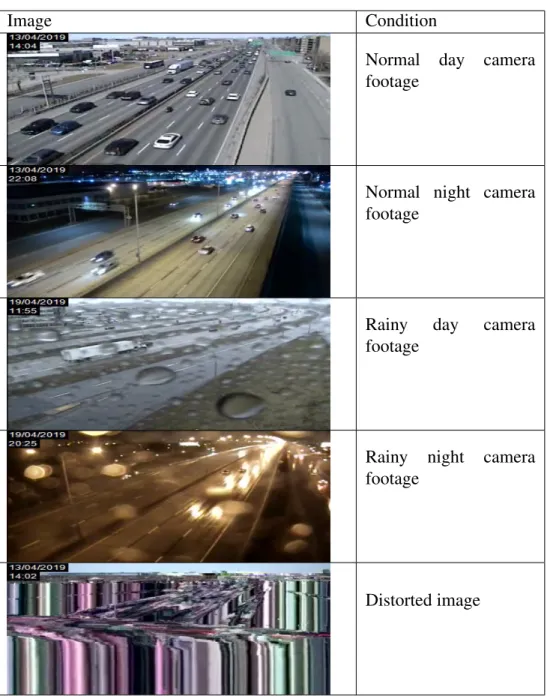
In figure 14, you can see some of the images which are collected from traffic cameras from different locations. There are around 42 traffic cameras in Autoroute 40, and the majority of them are functional 24/7. There is periodic maintenance, which makes the camera unavailable, and a message is shown instead of the footage. We collected images from these cameras every five minuets for five consecutive weeks and aggregated more than 400,000 images during this period. Later we divided the images into separate folders based on the date of the collected image to have a better-organized dataset.
Figure 13: Auto route 40. Courtesy of (Google-Maps, 2019)
Table 1 is the list of all the information we collected from the Quebec 511 website alongside all the images.
Data Description
Image The footage from the traffic camera Time The exact time of the current footage
Date The date of the current footage Address The location of the camera
Direction The direction which the camera is looking at Table 1: Collected Information from Quebec 511 website
4.4
Object Detection and Classification
In the previous section, we presented how we collected the images and mentioned that we collected more than 400,000 images for five weeks. It is a really time consuming and frustrating task for humans to count all the different vehicles in an image and repeat this task for the entire data set. In this section, First, we try to make sure that the data that we are dealing with is flawless and without any problem. Later, we explore the ways that we can automate the feature extraction task by applying different practices and algorithms to create a dataset containing the information extracted from the images.
4.4.1
Data Preparation
We collected images every five minutes, and more than 400,000 images were collected for five weeks. Since the environment that we are dealing with is a non-deterministic environment, we should expect different kinds of footage while we are collecting the data. However, most of the time, the images are without any noise or distortion. If the camera is under maintenance, no footage is shown, and instead, a message appears. Figure 15 indicates that there is a problem with the camera, and no footage is available.