Microarray Image Processing:
A Novel Neural Network Framework
Bachar Zineddin
School of Information Systems, Computing & Mathematics
Brunel University
Uxbridge, West London, UK
A thesis submitted for the degree of
Doctor of Philosophy
Dedicated to
My parents for all of their support over the years. My sons Safa, Wafa and Adam.
My wife Mera, her name should be next to mine on this thesis. Special thanks to my supervisors Prof. Zidong Wang and Prof. Xiaohui Liu.
Acknowledgements
I owe my deepest gratitude to my supervisors Professor Zidong Wang and Professor Xiaohui Liu for their enthusiastic guidance and advice throughout my research. Thank you for making the overall experience of my PhD most interesting. They have made available their support in a number of ways. I am indebted to many of my colleagues to support me; Dr Karl Fraser, Daniel Morris. I would like to thank all to all other colleagues in the IDA group. Finally, I would like to show my gratitude to Aleppo University (Syria), who through their funding opened up the possibility to begin with.
Abstract
Due to the vast success of bioengineering techniques, a series of large-scale anal-ysis tools has been developed to discover the functional organization of cells. Among them, cDNA microarray has emerged as a powerful technology that en-ables biologists to cDNA microarray technology has enabled biologists to study thousands of genes simultaneously within an entire organism, and thus obtain a better understanding of the gene interaction and regulation mechanisms in-volved. Although microarray technology has been developed so as to offer high tolerances, there exists high signal irregularity through the surface of the mi-croarray image. The imperfection in the mimi-croarray image generation process causes noises of many types, which contaminate the resulting image. These errors and noises will propagate down through, and can significantly affect, all subsequent processing and analysis. Therefore, to realize the potential of such technology it is crucial to obtain high quality image data that would indeed reflect the underlying biology in the samples. One of the key steps in extracting information from a microarray image is segmentation: identifying which pixels within an image represent which gene. This area of spotted microarray image analysis has received relatively little attention relative to the advances in pro-ceeding analysis stages. But, the lack of advanced image analysis, including the segmentation, results in sub-optimal data being used in all downstream analysis methods.
Although there is recently much research on microarray image analysis with many methods have been proposed, some methods produce better results than others. In general, the most effective approaches require considerable run time (processing) power to process an entire image. Furthermore, there has been little progress on developing sufficiently fast yet efficient and effective algo-rithms the segmentation of the microarray image by using a highly sophisti-cated framework such as Cellular Neural Networks (CNNs). It is, therefore, the aim of this thesis to investigate and develop novel methods processing mi-croarray images. The goal is to produce results that outperform the currently available approaches in terms of PSNR, k-means and ICC measurements.
Contents
Contents 4 List of Figures 8 Abbreviations 11 Publications 12 1 Introduction 1 1.1 Motivation . . . 21.2 Goal of The Thesis . . . 3
1.2.1 The State-of-the-art . . . 3
1.2.2 Thesis Contributions . . . 5
1.3 Overview of The Chapters . . . 6
2 Background 9 2.1 Introduction . . . 10
2.2 Molecular Biology . . . 12
2.2.1 The Structure of The DNA . . . 12
2.2.2 Central Dogma . . . 15
2.3 Microarrays Technology . . . 18
2.3.1 Introduction . . . 18
2.3.2 Gene Expression . . . 19
2.4 Microarray Experiment and Data Analysis . . . 20
2.4.1 Process Summary . . . 20
2.4.2 Experiment Design . . . 22
2.4.2.1 Choice of Sample Type . . . 22
2.4.2.2 Chip Fabrication . . . 22
2.4.2.3 Target Preparation and Labeling . . . 25
2.4.2.4 Biochemical Reaction (Hybridization) . . . 26
2.4.3 Image Acquisition and Data Readout . . . 27
2.5 Data Generation, Processing and Analysis . . . 28
2.5.1 Filtering . . . 28
2.5.1.1 Median Filter . . . 30
5 CONTENTS
2.5.1.3 Anisotropic Diffusion . . . 30
2.5.2 Gridding . . . 31
2.5.3 Segmentation . . . 31
2.5.3.1 Fixed Circle Segmentation . . . 32
2.5.3.2 Adaptive Circle Segmentation . . . 32
2.5.3.3 Histogram and Threshold Segmentation . . . 33
2.5.3.4 Adaptive Shape Segmentation . . . 33
2.5.4 Segmentation: Current State-of-the-art . . . 34
2.5.5 Background Separation . . . 36
2.5.6 Gene Quantification . . . 37
2.5.7 Microarray Data Analysis . . . 37
2.5.8 Microarray Image Reconstruction . . . 38
2.6 Testing Dataset . . . 39
3 A Novel Neural Network Approach for Microarray Image Segmentation 40 3.1 Classification . . . 41
3.2 Neural Networks . . . 42
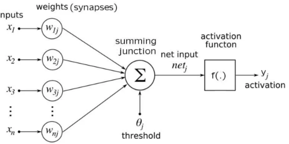
3.2.1 Artificial Neurons . . . 43
3.2.2 Activation Function . . . 45
3.2.3 Network Topologies . . . 50
3.2.4 Training of Artificial Neural Networks . . . 50
3.3 Multilayer Perceptron (MLP) Neural Networks . . . 51
3.3.1 FeedForward Neural Networks . . . 51
3.3.2 Hidden Layer . . . 54
3.3.3 Independent Validation . . . 54
3.3.4 Back-Propagation Algorithm (Delta Rule) . . . 55
3.4 Kohonen Neural Networks . . . 58
3.4.1 Self-Organizing Neural Networks . . . 58
3.4.2 Competitive Learning Algorithm . . . 59
3.5 Microarray Image . . . 60
3.6 The Proposed Approach . . . 61
3.6.1 Creation of Training Sets . . . 62
3.6.2 Single Neural Network Implementation . . . 63
3.6.3 Spot Classifier . . . 63
3.6.4 Multiple Neural Networks Implementation . . . 66
3.7 Experimental Results . . . 67
3.8 Conclusions and Future Work . . . 71
4 Adaptive Segmentation 74 4.1 Cellular Neural Networks . . . 76
4.1.1 Application Potential . . . 76
4.1.2 Architecture of Cellular Neural Networks . . . 77
4.1.3 Global Behavior of Cellular Neural Networks . . . 80
4.2 Nonlinear Diffusion Filtering . . . 81
6 CONTENTS 4.2.2 Isotropic Diffusion . . . 83 4.2.3 Anisotropic Diffusion . . . 84 4.2.4 Complex Diffusion . . . 86 4.3 Microarray Image . . . 87 4.4 The Framework . . . 87 4.4.1 Gridding . . . 88 4.4.2 Segmentation Algorithm . . . 88 4.4.2.1 Median 5x5 . . . 91 4.4.2.2 Anisotropic Diffusion . . . 91
4.4.2.3 The Median of ROI . . . 93
4.4.2.4 Two Channels to One Channel . . . 93
4.4.2.5 Local Threshold Estimation . . . 93
4.4.2.6 Locally Adaptive Segmentation . . . 94
4.4.2.7 SizeClass . . . 94
4.4.2.8 HoleClass . . . 95
4.4.2.9 GridClass . . . 95
4.4.3 Features’ Extraction . . . 95
4.5 Results and Evaluation . . . 96
4.5.1 The Peak Signal-to-Noise Ratio (PSNR) . . . 96
4.5.2 The k-means Objective Function . . . 96
4.5.3 The Objective Comparison . . . 98
4.6 Conclusions . . . 102
5 A Multi-View Analysis 105 5.1 Introduction . . . 106
5.2 Cellular Neural Networks . . . 108
5.3 The Algorithm . . . 108
5.3.1 Multi-View Analysis of cDNA Microarray . . . 109
5.3.1.1 Median Filter . . . 110
5.3.1.2 Top-Hat Filter . . . 110
5.3.1.3 Complex Diffusion Filter . . . 111
5.3.2 Segmentation . . . 111
5.3.2.1 Local Threshold Estimation . . . 111
5.3.2.2 Locally Adaptive Segmentation . . . 113
5.4 Main Results . . . 113
5.5 Conclusions . . . 115
6 A Novel Cellular Neural Network Approach for Microarray Image Seg-mentation 117 6.1 Nonlinear Mapping Using Cellular Neural Networks . . . 119
6.1.1 Introduction . . . 119
6.1.2 Chebyshev Approximation . . . 119
6.1.2.1 Chebyshev Nodes . . . 121
6.1.2.2 Data modeling . . . 122
7 CONTENTS
6.2 Multi-view Analysis: Dynamical Approach . . . 124
6.3 Microarray Image Analysis . . . 125
6.3.1 Initial Smoothing . . . 128
6.3.2 Background Trend Estimation . . . 129
6.3.3 Multi-view Curve Generation . . . 129
6.3.4 Adaptive Segmentation . . . 131 6.3.4.1 HoleClass . . . 131 6.3.4.2 SizeClass . . . 132 6.4 Discussion . . . 132 6.4.1 Testing Dataset . . . 133 6.4.2 Evaluation . . . 133
6.4.2.1 Non-linear Mapping Using CNN . . . 134
6.4.3 The Subjective Comparisons . . . 136
6.4.3.1 The Objective Comparison . . . 136
6.5 Conclusion . . . 137
7 A Cellular Neural Network for Microarray Image Reconstruction 141 7.1 Introduction . . . 142
7.2 Existing Techniques . . . 145
7.3 Novel Techniques . . . 146
7.3.1 Description . . . 146
7.3.2 CNNIR Algorithm . . . 147
7.3.2.1 The Pseudo-Code Of CNNIR (Fast-Inpainting) . . . 148
7.3.3 CNN-NSIR Algorithm . . . 149
7.3.3.1 Designing The Templates . . . 150
7.3.3.2 The Pseudo-Code of CNN-NSIR . . . 154
7.4 Discussion . . . 155
7.4.1 Notes About The Algorithms . . . 155
7.4.2 Dataset Characteristics . . . 156
7.4.3 Evaluation . . . 156
7.5 Conclusion . . . 159
8 Conclusions & Future Work 162 8.1 Introduction . . . 163
8.2 Achievements and Contributions . . . 164
8.2.1 Contribution 1: Total Automation and a Totally Blind Process . . . 166
8.2.2 Contribution 2: Adopting Local Strategy Algorithms . . . 166
8.2.3 Contribution 3: Image Filtering and Noise Reduction . . . 167
8.2.4 Contribution 4: Image Segmentation . . . 167
8.2.5 Contribution 5: Image Reconstruction . . . 168
8.2.6 Contribution 6: Cellular Neural Networks and PDEs Application . 168 8.3 Future Work . . . 169
List of Figures
1.1 The structure of thesis . . . 7
2.1 cDNA Microarray Image . . . 12
2.2 The structure of DNA . . . 13
2.3 X-ray diffraction image of DNA . . . 14
2.4 Chemical structure of DNA . . . 14
2.5 Ribonucleic Acid (RNA) . . . 15
2.6 The Codon . . . 16
2.7 Informotion flow inside the biological cell . . . 17
2.8 An overview of a microarray experiment . . . 21
2.9 Nylon-slide Microarray . . . 23
2.10 Oligonucleotides Microarray . . . 25
2.11 Gene spot background separation . . . 37
3.1 The model of an artificial neuron . . . 44
3.2 Linear activation function . . . 45
3.3 Symmetric hard limiter activation function . . . 46
3.4 Symmetric saturating linear activation function . . . 46
3.5 Binary sigmoid activation function. . . 47
3.6 Hyperbolic tangent sigmoid function. . . 48
3.7 Derivatives of hyperbolic tangent and binary sigmoid functions. . . 49
3.8 A linear decision boundary . . . 49
3.9 A multi-layer neural network architecture . . . 53
3.10 Two-channel cDNA microarray image . . . 61
3.11 Microarray image processing steps . . . 63
3.12 The architecture for the competitive later. . . 64
3.13 Spot classifier. . . 65
3.14 9 classes of spots determined by the network. . . 65
3.15 The proposed network architecture . . . 67
3.16 Microarray image sample input . . . 67
3.17 Example of the MLP segmentation algorithm output. . . 68
3.18 Comparison of segmentation results . . . 68
3.19 NN Segmentation Results - training image . . . 70
9 LIST OF FIGURES
4.1 A 2-dimensional CNN defined on a squared grid. The ij-th cell of the array is colored by black, cells that fall within the sphere of influence of
neighborhood radius r= 1 (the nearest neighbors) by blue . . . 77
4.2 A CNN base cell circuit . . . 78
4.3 A block diagram representing CNN . . . 79
4.4 A piecewise-linear function, CNN cell output function . . . 80
4.5 The filtering mask of size 3×3 . . . 81
4.6 Microarray image analysis . . . 88
4.7 Microarray segmentation algorithm . . . 90
4.8 SizeClass algorithm . . . 94
4.9 PSNR for the Dataset. Comparison of segmentation results between GenePix (GP), Median, Diff1, Diff2 and CDiff (CLD) algorithms. . . 97
4.10 k-means for the Dataset. Comparison of segmentation results between GenePix (GP), Median, Diff1, Diff2 and CDiff (CLD) algorithms. . . 98
4.11 Examples of the PSNR and k-means values for a spot . . . 99
4.12 Average within-spot estimated variance over the dataset. Comparing be-tween GenePix (GP), Median, Diff1, Diff2 and CDiff (CLD) algorithms. . . 101
4.13 Average between spot estimated variance over the dataset. Comparing be-tween GenePix (GP), Median, Diff1, Diff2 and CDiff (CLD) algorithms. . . 101
4.14 Comparing the results of the proposed adaptive segmentation algorithms. ICC over the dataset . . . 102
5.1 Pipeline of multi-view feature response curve generation . . . 110
5.2 Locally adaptive segmentation with median and top-hat filters . . . 112
5.3 Locally adaptive segmentation with complex diffusion filter . . . 112
5.4 The percentage of accuracy for different filters . . . 114
5.5 PSNR for the Dataset . . . 115
6.1 Adaptive Mulit-View Analysis AMVA algorithm . . . 126
6.2 Adaptive segmentation algorithm . . . 126
6.3 An example of microarray image block (green and red channels) will be used to demonstrate the output of each stage in the algorithm . . . 127
6.4 The output of filtering stage for the block example presented in Figure 6.4 130 6.5 Segmentation results for the green and red channels in Figure 6.4 . . . 132
6.6 Block 6.4’s final output . . . 133
6.7 (a) sqrt represents the approximated function y = √x; (b) pwl represents the results of the improved algorithm; and (c) pwl N is the results of the original algorithm using the same segment number that is suggested in (b) 135 6.8 psnr . . . 136
6.9 k-means . . . 137
6.10 Within-spot estimated variance σ2 e . . . 138
6.11 Between-spots estimated variance σ2 g . . . 138
10 LIST OF FIGURES
7.1 Part of a microarray image gives a good example of the variations in the background signal. The target is to reconstruct the areas of the spots, the bright circles signals, assuming that there is no information in these areas
(‘0′s) . . . . 144
7.2 Gene spot background region as used by common packages: 1) GenePix; 2) ImaGene; 3) ScanAlyze . . . 145
7.3 Output sample by applying diffusion template on Ω region . . . 148
7.4 Output sample by applying CNNIR algorithm on Ω region . . . 149
7.5 Reconstructed images using CNN-NSIR algorithm . . . 155
7.6 Within-Spot estimated variance over the dataset. (The methods are ‘No Background Correction’, ‘Median Background Estimation’, ‘Bertalmio’, ‘CNN-NSIR’ and ‘CNNIR(f-Inpaint)’. . . 157
7.7 Between-Spots estimated variance over the dataset. (The methods are ‘No Background Correction’, ‘Median Background Estimation’, ‘Bertalmio’, ‘CNN-NSIR’ and ‘CNNIR(f-Inpaint)’. . . 158
7.8 Average ICC over the dataset. (The methods are ‘No Background Cor-rection’, ‘Median Background Estimation’, ‘Bertalmio’, ‘CNN-NSIR’ and ‘CNNIR(f-Inpaint)’. . . 158
7.9 Boxplot for one sample gene. . . 159
Abbreviations
AI ArtificialIntelligence ANN ArtificialNeural NetworkBP BackProbagation
cDNA complementary DNA CNN Cellular Neural Network CNN-UM CNN- Universal Machine CC Copasetic Clustering CLD Complex Diffusion
DIP Digital Image Prpcessing DNA DeoxyriboNucleic Acid ESTs ExpressedSequence Tags FFT Fast Fourier Transform
FPGA Field-ProgrammableGate Array GMM Gaussian Mixture Model
GP GenePix
GPU Graphics Processing Unit ICC IntraClass Correlation IDA Intelligent Data Analysis LD Linear Diffusion
LMS Least Mean textbfSquare MLP MultiLayer Perceptron
mRNA messenger RNA
MSE Mean Square Error
NIH National Institutes of Health NSE Navier Stokes Equation PCR Polymerase Chain Reaction PDE Partial Differential Equation PDP Parallel Distributed Processing PSNR Peak Ssignal to Nnoise Ratio PWL PieceWise Linear
RNA RiboNucleic Acid
SCIR graphS-CutImage Reconstruction SOM Self-Organizing Map
SRG Seeded Region Growing TIFF Tagged ImageFileFormat
Author’s Publications and
Presentations
Some of the new work presented in this thesis has been previously published/submitted for publication.
Chapter 3 Zineddin, B., Wang, Z. & Liu, X., 2010. A Novel Neural Network Ap-proach To cDNA Microarray Image Segmentation. Pattern Recognition Letters, submitted.
Chapter 4 Zineddin, B., Wang, Z. & Liu, X., 2010. cDNA Microarray Segmen-tation: Adaptive Approach. IEEE Transactions on Image Processing, Submitted.
Chapter 5 Zineddin, B., Wang, Z. & Liu, X., 2010. A Multi-View Approach to cDNA Microarray Analysis. International Journal of Computational Biology and Drug Design, 3(2), pp. 91-111.
Zineddin, B. et al., 2008. Investigation on Filtering cDNA Microarray Image Based Multiview Analysis. In S. Zhang & D. Li, eds. Proceeding of the 14th International Conference on Automation & Computing. London, UK: Pacilantic International Ltd., pp. 201-206.
Chapter 6 Zineddin, B., Wang, Z. & Liu, X., 2010. A Microarray Image Multiview Analysis Based on Cellular Neural Network. IEEE Transactions on Neural Networks, Submitted.
Chapter 7 Zineddin, B., Wang, Z. & Liu, X., 2010. Cellular Neural Networks, Navier-Stokes Equation and Microarray Image Reconstruction. IEEE Transaction On Image Processing, Revised.
Zineddin, B., Wang, Z. & Liu, X., 2010. Cellular Neural Networks, Navier-Stokes Equation and Microarray Image Reconstruction. In IEEE International Conference on Bioinformatics and Biomedicine Workshops (BIBMW). HK, pp. 234-239.
Zineddin, B., Wang, Z. & Liu, X., 2010. A Cellular Neural Network for Microarray Image Reconstruction. In Proceedings of the 16th Inter-national Conference on Automation & Computing. Birmingham, UK, pp. 106-111.
Chapter 1
Introduction
Chapter 1. 2 Introduction
1.1
Motivation
Arguably, the conquest of the unknown is the best description of human history during the last few millenniums, which is the most startling one despite all other aspects of this history. It is the journey of human to understand the life, themselves and their relation to the universe. Through several thousands of years many schools of thoughts have tried to give the right answer; or at least give a pathway to approach this answer. Starting from the far east Taoism, Indian Buddhism, Mesopotamia and ancient Egypt civilizations, through the Greek and their recent descendants, the Islamic and the last surviving, West civilizations, everyone has its own set of rules that shape these pathways.
Regardless of all the past discoveries which are parts of a long debate about accepting them as myths or mere other point of view of the same reality, it is the most sparkling milestone achievements, which have been attained during the last two centuries by some great minds in the human history, that will be the basis for this current study.
Starting from Gregor Mendel, who can be considered as the father of the modern genetics, although his work stayed obscure until the beginning of the twentieth century, to the most astonishing discoveries in the last century, the chromosomes, the structured of the Deoxyribonucleic Acid (DNA) and the rules of the genetic material within the living cell have been discovered.
Within the last thirty years, many developments have been achieved and our under-standing of biology of the living systems has started to build up in wide steps. However, most of these advances until mid nineties were limited to the ability to sequence the DNA. A little has been done to improve the methods that allow human to grasp a deep insight about the functions of the genes and the relations within the genetic material and between these materials and the surrounding environment. Within this context, the microarray technology appeared as an effective throughput technology for functional genomics.
With the introduction of this technology, a new era has begun. The huge data that have been resulted from just a few experiments led to the whole novel techniques within the data analysis methodology to cope with the high demand of such outputs. The developed techniques covered many study areas from the data storage management tools, Intelligent Data Analysis (IDA), to Digital Image Processing (DIP) and many more.
The analysis of the microarray image, though it might seem an easy and straightforward task, is a difficult and challenging problem. Therefore, it is our aim in this thesis to tackle this issue by developing and applying up-to-date techniques that merge many highly potential ideas from various disciplines such as Artificial Neural Networks (ANNs), Partial Differential Equations (PDEs) and Linear Diffusion (LD) filtering techniques.
Chapter 1. 3 Introduction
1.2
Goal of The Thesis
1.2.1
The State-of-the-art
Due to the recent success of bioengineering techniques, many large-scale analysis tools have been developed to investigate the functional organization of the cell. Among them, cDNA microarray has emerged as a powerful technology that enables biologists to study thousands of genes simultaneously within an entire organism and, thus, to obtain a better understanding of the genes’ interaction and regulation mechanisms involved. However, this technology is still in the beginning of getting its potentials, and lots of improvements are required in all the stages of the microarray process.
Although microarray technology has been developed so as to offer high tolerances, there exists large signal irregularity through the surface of the microarray image. The imperfection in the microarray image’s generation process causes noises of various types, which contaminate the resulting image. These errors and noises will propagate down through, and can significantly affect, all subsequent processing and analysis. Therefore, to realize the potential of such technology it is crucial to obtain high quality image data that will indeed reflect the underlying biology in the samples. One of the key steps in extracting information from a microarray image is the segmentation with aim to identify which pixels within an image represent which gene. This area of spotted microarray image analysis has received relatively a little attention comparing to the advances in proceeding analysis stages. This attitude towards image analysis was in part due to first, the believe that this stage has little impact on the later stages and, second, the need for multi-disciplinary knowledge was crucial to build effective and efficient algorithms. It is worth pointing out that the lack of advanced image analysis including the segmentation results in sub-optimal or even poor quality data being used in all downstream analysis methods.
Some of the research papers, which have played an essential role in the development of proposals presented in this thesis, are now discussed as follows.
Arena et al. [2002a] proposed a real-time algorithm to process the microarray image using the Cellular Neural Network (CNN) array. The CNN is an analogic processor array [Chua & Roska, 1993b; Chua & Yang, 1988b,d] that allows the application of a local strat-egy, with less computational complexity, to meet the task requirements. It is important to note that using spatial information leads to a robust and reliable algorithm in some ap-plications such as microarray image analysis. Due to its architecture, the two dimensional CNN array is widely used to solve image processing and pattern recognition problems. Furthermore, the parallelism of this structure allows one to perform the most computa-tionally expensive image analysis tasks faster than the classical CPU-based computer does.
Chapter 1. 4 Introduction
Essentially, the algorithm in [Arena et al., 2002a] used two colors, red and green. The first step consists of filtering operations; this process cleans the background noise and removes the ill-positioned spot. The next step is to remove patches and irregular size spots. After these operations, the following phase addresses the intensity analysis of both channels.
In [Samavi et al., 2004], a pipeline architecture was designed particularly for real-time and semi-parallel microarray processing. This architecture, first, produces a binary map using a threshold value. Then, the map goes through gridding and morphological operators. Next, the masking operator assigns the original gray scale value to pixels that have 1’s in the map. The last step is the intensity analysis; image is compared with a number of thresholds to the intensity level of each spot.
Hirata et al.[2002] presented a technique based on mathematical morphology that per-forms the segmentation. The procedure of image segmentation consists, basically, of: 1) Creating one gray-scale image from the red and the green images; 2) Rotation correction; 3) Sub-array and spots gridding; and 4) Spot segmentation. The segmentation stage, in particular, takes both the morphological gradient of the filter image and a marker image, which is composed of the approximated centers of the spots and the grid itself. Then, a wa-tershed operator [Beucher, 1982; Soille & Vincent, 1990; Vincent & Soille, 1991] should be applied with a basic cross structuring element. Another algorithm based on mathematical morphology was proposed in [Angulo & Serra, 2003]. In this algorithm, initially, a gridding algorithm automatically produces spots’ quadrants, which will be analyzed individually in later stages. Then, the analysis of the spot quadrant images is achieved in five steps includ-ing spot size estimation, background noise extraction, spot position determination, spot boundary definition which is carried out using the watershed transformation and, finally, spot signal quantification. Siddiquiet al. [2002] applied another algorithm to carry out the segmentation process that is based on mathematical morphology and watershed technique, followed by quantification of the shapes of the segmented spots using B-Splines [Cohen
et al., 2001].
Fraser [2006] proposed many mapping functions that place emphasis on certain fre-quencies or regions of interest. This methodology would not only be advantageous but also be more effective in terms of the overall goal. These functions are named as inverse, a summed inverse and square root, a square root and a linear function. For instance, if the image is first filtered using the inverse function to emphasize the genes, the clustering output is improved dramatically. Similarly, photographic polarizing filter allows details normally hidden behind reflections to be captured. Therefore, filtering the image in this way allows us to analyze details that would otherwise be lost.
Chapter 1. 5 Introduction
1.2.2
Thesis Contributions
Recently, much research on microarray image’s segmentation with many methods has been proposed, some methods produce results better than others. In general, the most effective approaches require considerable run time (processing power) to process an entire image. Furthermore, there has been little progress in developing sufficiently fast yet efficient and effective algorithms for the segmentation of a microarray image by using up-to-date tech-niques such as Artificial Intelligence (AI) approaches, specifically neural networks. It is, therefore, the aim in this thesis to investigate and develop novel analyzing methods for mi-croarray images. In other words, our goal is to produce results that outperform the results of currently available approaches in terms of robustness, effectiveness and time efficiency. The following issues will be investigated in this thesis:
1) Fully Automation: The large number of spots, usually in thousands, as well as the shape and position irregularities [Lukacet al., 2005; Wanget al., 2003b] can propagate processing errors through subsequent analysis steps [Eisen & Brown, 1999; Lukac et al., 2004; Wang et al., 2003a]. Furthermore, the time-consuming manual processing of the microarrays has led to the interest in using a fully automated procedure to accomplish the task [Bajcsy, 2004; Jainet al., 2002; Katzer et al., 2003]. Automatic algorithm guarantees the elimination of user’s errors and is considered as an essential step towards a unified framework for microarray image analysis.
2) Local Strategy: Considering the signal variability across the microarray image, the emphasis will be placed on techniques that benefit from the local information in order to achieve different tasks in the image analysis process. Therefore, it can be assumed that the global image properties are irrelevant and, rather, a locally adaptive strategy with less computational complexity can meet the application requirements.
3) Image Filtering: The system imperfections and the microarray generating process restrict our ability to differentiate between spots signals and background signal as well as our ability to get accurate measures of interest in the images. Therefore, it makes much more sense to produce filtered versions of the image data so that the dynamic range of the image can be increased, and hence a better ability of signal extraction could be achieved.
4) Multi-view Analysis: The mapping functions, proposed in Fraser [2006], will be investigated thoroughly in order to draw a full understanding of their effects on the image analysis process. In addition, the ability to approximate these functions in any possible hardware implementation will be addressed.
5) Image Segmentation: It has been anticipated that the spot intensity value would be independent of the segmentation algorithm if a background correction method is utilized [Yang et al., 2002]. However, Lehmussola et al. [2006] showed that even with a correction
Chapter 1. 6 Introduction
procedure the segmentation method will significantly influence the identification of differ-entially expressed genes. Therefore, investigating the segmentation process will occupy a considerable part of this thesis.
6) Image Reconstruction: Considering the inherent variation between the gene and background regions, image reconstruction is one of the best techniques that can be applied to estimate the local background of every spot. By the end of this thesis, some of the most popular reconstruction techniques for the general imagery will be adopted to be applied on the microarray image.
7) PDE: The filtering techniques based on PDEs will be investigated in order to, first, benefit from their potential in the image processing applications; second, utilize the fact that PDEs can be used to build hardware architectures which approximate successfully these systems.
8) CNN: The ultimate goal of this study is to draw a road map toward a fully auto-mated and parallel hardware implementation of the image processing steps. CNN is one of the best options to achieve this goal. Due to its architecture, the two-dimensional CNN array is widely used to solve image processing and pattern recognition problems. Further-more, the parallelism of this structure allows one to perform the most computationally expensive image analysis tasks faster than they do in classical CPU-based computer.
1.3
Overview of The Chapters
Figure 1.1 gives a general view about the thesis structure. In the next chapter the back-ground review of our research is presented. Chapter 2 covers the the underlying biology behind the microarray technology, the development that led to this high throughput tech-nology, conducting the microarray experiment and, finally, a comprehensive review of the microarray image processing.
In Chapter 3, we will propose a new segmentation method utilizing a series of Multi-Layer Perceptron (MLP) and Kohonen neural networks. The presented networks have a new structure that is particularly suitable to the task at hand.
In Chapter 4, the image is filtered by applying a nonlinear anisotropic diffusion with several diffusion functions in order to increase the dynamic range of the image, and thus to increase the ability to extract desired signals. The proposed novel algorithm is based on the CNN computational paradigm integrated with median and anisotropic diffusion filters. The investigation, in Chapter 5, is to improve the processes involved in the analysis of microarray image data. The main focus is to clarify the image features’ space in an unsupervised manner. Instead of using the raw microarray image, it is suggested that
Chapter 1. 7 Introduction
Chapter 1. 8 Introduction
producing multiple views of the image data, i.e. highlighting certain frequencies, will yield more reliable results in the filtering stage. In addition, this methodology will be advantageous for the segmentation stage and the system as a whole. Therefore, the multi-view analysis framework is combined with many filters such as Median, Top-Hat and Complex Diffusion (CLD). Then, a thorough analysis is conducted to understand the effects of these filters on the segmentation stage.
In Chapter6, an automatic and non-supervised algorithm for a fast and accurate pixels’ classification is presented. The proposed approach in this chapter follows two lines: first, the development of CNN algorithm to approximate any mapping function and, second, the integration of diffusion based filter with an adaptive segmentation algorithm. The main advantages of this approach are that it establishes a general framework that can make the whole cDNA microarray technology fully parallel as well as it minimizes the processing time.
Two new image reconstruction algorithms based on CNN are proposed in Chapter 7. The presented methods tend to get an exemplary approximation of the background in the gene spot region either by using diffusion based algorithm or by solving the Navier-Stokes equation. These algorithms offer robust methods to estimate the background signal within the gene spot region. Subtracting this reconstructed background from the original image should lead to a more accurate quantification of genes’ signals.
Chapter 2
Background
Chapter 2. 10 Background
Imagine watching a play with thirty thousand actors. You’d get pretty confused.
James Watson
2.1
Introduction
Certainly, Gregor Johann Mendel’s results can be considered as a major milestone in the quest to understand the nature and the content of genetic information, though the theo-retical realization of the genetics was not yet extended by momentous ideas that have to be presented in the twentieth century. Although Mendel did not know the physical units that represent the genetic information, his experiments showed quantitatively how to pre-dict the underlying inheritance. His work, therefore, established a theory to explain this heredity based on assumed factors; we can now understand them as genes. Unfortunately, Mendel’s paper, “Experiments in Plant Hybridization”, had been ignored until many sci-entists rediscovered his conclusions and cited it at the beginning of the 20th century.
In the following decades, many milestone achievements can be specified: 1) Chromo-some was discovered and the relation between the heredity, development and the chromo-somes have gradually become significantly evident. 2) Then, as a major breakthrough, Watson & Crick [1953] revealed the molecular basis of the heredity, the DNA double helix. 3) The next astonishing establishment was unlocking the informational basis of heredity. 4) The biochemical studies, which were carried out during 1950s by a group of physicists and chemists [Robertset al., 1955], uncovered the basic mechanisms involved in the regulations of metabolic pathways. 5) The invention of the recombinant DNA technologies of cloning and sequencing [Kleppe, 1971], with the knowledge of the biological mechanism, enabled the scientists to read the genetic information.
In 1990, the National Institutes of Health (NIH) introduced a new method to accelerate the gene discovery [Adams et al., 1993]. Molecules, which are called Expressed Sequence Tags (ESTs) and evolved from the development of Complementary DNA (cDNA), provide scientists with a quick and inexpensive tool for gene identification, gene expression and genome mapping [Gerhold & Caskey, 1996; Marra et al., 1998; McLachlan et al., 2004; Quackenbush, 2001]. Mapping genes and sequencing DNA enable researchers to draw conclusions about the gene function from its structure. In addition, the sequencing of specific genome offers a direct access to genome molecules using the Polymerase Chain Reaction (PCR). With these sequences, biologists will be able to design primers, which
Chapter 2. 11 Background
can amplify a particular DNA fragment, or they can effectively screen a library for a larger segment of DNA containing the region of interest. Furthermore, sequencing increases the ability to search efficiently for similar genes in other organisms.
The (PCR) [Rabinow, 1997] and automated DNA sequencing technologies [Hegdeet al., 2000] were remarkable achievements. While the PCR methodologies allowed researchers to amplify a very small amount of DNA, the automated DNA sequencing approach enhances the ability to obtain the entire DNA sequence of microbial genomes within few days. These achievements have initiated the human genome project [Gene, 1999]. The PCR, as an amplification tool, is an important part of DNA analysis for many reasons: 1) It provides a method to an essentially limitless supply of material. 2) The PCR is a procedure that uniformly amplifies the sample so this sample will not be altered, distorted, or mutated by the process of amplification. 3) Another rationale behind DNA amplification is the amplification selectivity of a region which is an easy way to purify that segment from the bulk. With sufficient amplification magnitude, the DNA product becomes such a major material of the amplification mixture; i.e., the starting sample is reduced to a sufficiently small percentage for most applications.
Scientists devote their efforts to sequence and assemble the genomes of various or-ganisms, especially the human [Lander et al., 2001; Ledford, 2007; Wheeler et al., 2008]. However, genome sequencing is merely the transfer of the information contained within the DNA which serves as the repository of the genetic information, to another carrier. Genome sequencing provides raw data which does not provide a way to get what the data means or how the data can be utilized in various clinical applications. On the other hand, besides obtaining a genomic sequence and specifying a complete set of genes in any sequencing project, the ultimate goal is to get an understanding of the functionality of this genetic information. In other words, gaining insight about the function of a specific gene or set of genes in the normal circumstances increases our ability to understand the deceased situations. Investigating the relationships among genes in the DNA is another major goal in molecule biology [Cohen, 2005]. This new field of study, which is known as functional genomics, led to the emergence of new high throughput technologies that al-lowed researchers to tackle difficult problems and reveal promising solutions in many fields, i.e. cancer research [Ley et al., 2008].
DNA microarray is a remarkably successful high throughput technology for functional genomics [Schenaet al., 1995; Shalonet al., 1996]. Microarrays allow researchers to analyze the expression level, in different cell types or conditions, of many thousands of genes in a single experiment [Alizadeh et al., 2000; Moore, 2001]. Basically, a DNA array [Stekel, 2003] can be defined as an orderly arrangement of tens to hundreds of thousands of unique
Chapter 2. 12 Background
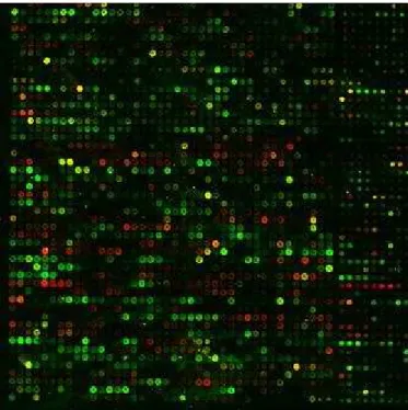
DNA probes of known sequence. The probes, which are either individually synthesized on the array surface or pre-synthesized by a procedure such as PCR, are attached to the array platform. The cDNA microarray aim to detect the abundance of various mRNA molecules of a cell by using hybridization of the fluorescent labeled samples to the DNA probes already existed on the array [Schena et al., 1995]. This abundance can provide information about the related protein or the expressed gene [Gygi et al., 1999]. The end product of the cDNA microarray experiment is a scanned array image, see Figure 2.1, [Moore, 2001; Orengo et al., 2003]. These images must then be analyzed to identify the arrayed spots and measure the relative fluorescence intensities for each feature.
Figure 2.1: cDNA Microarray Image
2.2
Molecular Biology
2.2.1
The Structure of The DNA
By the early beginning of the 20th century, Mendel’s works have become widely known [Klug & Cummings, 2003] and got fully credited by Bateson [Bateson, 2007]. A couple of years later, Sutton [1903] suggested the applicability of the Mendelian laws of inheritance to chromosomes. Sutton suggested that chromosomes contain units (“genes”) which affect the heredity and the development. Furthermore, he showed that meiosis, the process by which the genetic material of eukaryotic cells is duplicated and distributed during cell division,
Chapter 2. 13 Background
gives a mechanism for Mendelian inheritance. Two decades later, the experiments of T.H. Morgan [Allen, 1978] on the fruit fly verified Sutton’s hypothesis. Yet, the genes, their roles or how they produce physical features in organisms, were still to be discovered years later.
The discovery of the nucleic acid in the 19thcentury by the biologist Friedrich Miescher [Allen, 1978] marked an important step toward a more advanced understanding of the heredity in the last century. By the late 1920s, chemists had discovered both ribonucleic acid (RNA) and deoxyribonucleic acid (DNA). Levene [1919] investigated the structure and the function of the nucleic acids and highlighted different forms of them, namely the DNA and RNA. However, the connection of nucleic acids with genes was yet to be established a decade later [Lorenz & Wackernagel, 1994]. The studies, back then, showed that the chromosomes contain DNA, which is suspected to be the genes’ material. By the end of 1940s, DNA is proven to be the right answer, and this was finally determined experimentally.
Figure 2.2: DNA structure.
Zygote Media Group.
The biggest breakthrough came when Watson & Crick [1953] proposed a model of double helix as the structure of the DNA, see Figure 2.2. This model is accepted now
Chapter 2. 14 Background
as the first correct structure of DNA. The model of DNA was based on a single X-ray diffraction image, which was called “Photo 51” and introduced in [Franklin & Gosling, 1953], see Figure 2.3. Those findings led to the proposal of the Central Dogma of the molecule biology, which describes the relation between DNA, RNA and proteins [Crick, 1955]. Soon later, Meselson & Stahl [1958] confirmed the replication mechanism that was implied by the double helix model.
Figure 2.3: This image is a faithful digitalization of the famous historic photograph Photo 51, the name is given to an X-ray diffraction image of DNA introduced in [Franklin & Gosling, 1953]. http://en.wikipedia.org/wiki/File:Photo_51.jpg
Figure 2.4: Chemical structure of DNA. Hydrogen bonds shown as dotted lines.
Madeleine Price Ball.
DNA is the basic hereditary material in all cells and contains all the necessary infor-mation to make proteins. DNA is a linear polymer made up of nucleotide units. The
Chapter 2. 15 Background
nucleotide unit consists of a base, a deoxyribose sugar and a phosphate, see Figure 2.4. There are four types of bases: adenine (A), thymine (T), guanine (G), and cytosine (C). In DNA, the bases are perpendicular to the helix axis and form pairs: A to T and G to C. This relation is called a complementarity and contributes to the determination of the whole DNA shape, which gives a high robust reproduction of the basis sequence in the DNA chain. This invariant relation is used in the cell to duplicate the DNA during cellular reproduction and in protein synthesis. The double helix of DNA can be divided into two helices and then recomposed with a process called hybridization. Each specific protein is built starting from a specific DNA sequence within the whole DNA chain, called a gene. RNA chemicals are very similar to the DNA ones. However, there are some differences, RNA contains uracil (U) instead of thymine (T), RNA is a single stranded and finally RNA contains ribose sugar instead of deoxyribose sugar, see Figure 2.5.
Figure 2.5: Ribonucleic Acid (RNA).National Institute of Health
2.2.2
Central Dogma
The genetic information is stored in the DNA strands. Segments of these strands encode genes. Generally, each gene produces a particular protein by coding each of the amino acids that make up the protein. Every amino acid is encoded by three nucleotide bases, for instance, the nucleotides “AAG” correspond to the amino acid phenylalanine. This three-letter code is called a codon, see Figure2.6. In order to understand the process of producing proteins from genes, central dogma of molecular biology should be considered. Briefly, genes are transcribed into messenger RNA (mRNA) and mRNA, and then translated to form
Chapter 2. 16 Background
proteins, which are the building blocks and functional elements of any living cell. Gene’s expression is the indication of the presence of this mRNA.
Figure 2.6: The codon. National Institute of Health
Figure 2.7 shows the genetic information flow inside the cell. The first step is the transcription which happens in the cell nucleus. From a single strand of the DNA, a protein, also called enzyme, sets the strands apart in a small section of the DNA. This enzyme then uses one of the DNA strands to create the mRNA molecule by a letter-for-letter copy of this section; i.e., in every place where the gene has (C), the mRNA has (G), and in every place where the gene has (A), the mRNA has (U). Therefore, the RNA molecule transcribed from the gene is complementary to the coding strand of that gene.
The stability is a main character of DNA. The same copy of genomic DNA exists almost in all the cells of an organism. Yet, cells are different in shape and function. These differences between them are due to the different subsets of expressed genes in each of the different cell types. In addition, different stimuli provoke different subsets of genes to be expressed. Thus, the pattern of gene expression levels reflects both the cell type and its condition. Microarrays allow researchers to detect the abundance of various mRNA molecules or transcripts in a cell at a given moment. Although the relation between the abundance of mRNA and the corresponding protein is not necessarily straightforward [Gygi
et al., 1999], it is accepted that the quantity of each mRNA detected in the cell can provide
information on the corresponding protein.
One example that reflects how important it is to characterize protein construction is that many human diseases are due to the failed synthesis of a particular protein; for
ex-Chapter 2. 17 Background DNA mRNA (abundance can be detected using microarrays) Protein Cell structure Replication Repair Metabolism . . . . . . Transcription Translation Regulation of gene expression
Figure 2.7: The information transfer between DNA, mRNA and protein (the ”central dogma”). Segments of DNA are used as a code to make mRNA, which is used as a code to make protein. Microarray experiments exploit the relation between mRNAs and the genes that encode them.
ample, insulin. The target here is to induce specific micro-organisms such as bacteria to synthesize that specific protein. Here, the first step is to know which gene is responsible for the production of the desired protein. After that, the selected gene is inserted into the micro-organism obtaining a kind of protein factory. Another example is the impor-tant exploration field that involves the study of the so-called oncogenes; i.e. genes that when mutated or expressed at abnormally high levels contribute to the conversion of a normal cell into a cancer cell. Furthermore, in [Evans, 1999], mutations in genes are used as important determinants of drug effects, which represents a key issue in the emerging pharmacogenomics discipline. These are only few examples of the huge possibilities that can be derived from the discovery, characterization and recognition of genes.
Every protein is formed from a specific sequence of the 20 amino acids. Their dis-placement information is transferred from the DNA through a translation code formed by a subsequence of three bases of nucleotides. So, each amino acid relates to a specific sequence of three bases, the codon. Therefore, in the classification of proteins, the major issue to be unraveled is to discover, for each protein, the sequence of bases that generated it. When a particular gene codifies a protein, it is said to be expressed into the protein. Since even the most powerful microscope is unable to distinguish among genes, new methodolo-gies are required to gain the global gene expression profile. Many laboratories are working to make a database of gene structures as soon as they are discovered.
Chapter 2. 18 Background
2.3
Microarrays Technology
2.3.1
Introduction
Microarray technology came on time to cover the need to monitor in parallel all the DNA sequences and to have the adequate sensibility to detect the variation of gene expression. Furthermore, this technology affects the data volume that can be acquired during a limited time. The crucial impact of facilitating this technology was the boost of our understanding of organisms and various biological processes. During 1990s, some parallel methods have been introduced, allowing the possibility to detect the expression level of a huge number of genes simultaneously. The first method, devised in the laboratory of Pat Brown at Stanford [Schena et al., 1995], is based on the robotic micro-deposition and the fixing of DNA single-stranded fragments in microarrays mounted on microscope slides with a size of 2 cm×2 cm. The second method depends on the high density spatial synthesis of oligonucleotides [Lipshutz et al., 1999]. Other methods depend on the development of in situ synthesis with reagents delivered by ink-jet printer devices [Hugheset al., 2001].
The development of microarray technology and its success are sparked by the intro-duction of many innovations in recent decades. The highly specific preferential binding of complementary single-stranded nucleic acid sequences was first exploited experimentally in the mid 1960s. This method achieved a remarkable success in the form of a technique which is called the Southern blot [Gillespie & Spiegelman, 1965; Southern, 1975]. Some other innovations are the progress in the genome sequencing, the advances in miniatur-ization and the high density synthesis of nucleic acids on non-porous solid supports, such as glass, nylon or silicon. Microarrays were first used to study global gene expression in [DeRisiet al., 1997].
Remarkably, the microarray technique represents a real breakthrough in biological and medical fields, since all traditional gene expression detection methods provide gene in-formation in a sequential way. The availability of genes’ data-bases enables researchers to study all the genes belonging to a given organism simultaneously. Therefore, the researcher will obtain a quantitative information about cellular pathways and will observe the effect of different physiological conditions on such pathways by direct comparison between the expression levels of the genes. Microarray has already been facilitated in a wide range of applications; notably, for novel gene discovery, expression profile analysis, drug discovery and development, investigating biochemical pathways, diagnostics, therapeutics and pro-teomics [Holloway et al., 2002; Leung & Cavalieri, 2003; Samartzidou et al., 2001; Schena
Chapter 2. 19 Background
2.3.2
Gene Expression
Gene expression is highly valuable for exploring genetic regulations such as investigating metabolism. In addition, investigation of gene expression forms a very effective method-ology in the molecular medicine such as classification of disease, diagnosis, prognostic prediction and in a number of industrial and pharmaceutical applications [Cohen, 2005].
Maybe it is a common observation that biologists have found many genes to be co-regulated [Eisen & Brown, 1999; Eisen et al., 1998] in an extremely efficient way. Co-regulation under various biological conditions means that there is a relative similarity among the corresponding expression profiles [Chou et al., 2007]. These genes include the genes of nutrition, stress responses and metabolic pathways. Some other co-expressed genes are the genes encoding the ribosome, the proteosome and the nucleosome [Alon, 1999; Brown & Botstein, 1999; Caustonet al., 2001; Eisenet al., 1998; Hugheset al., 2000; Lashkari et al., 1997].
The gene expression profile is the measurements of gene expression of the genes under study. Therefore, it can be considered as a representation of the molecular definition of a cell in a specific state [Young & Center, 2000]. Obtaining adequate information about the transcriptional profile of biological sample is very important. Expression profile is a way for describing a phenotype, which can be a complete set of observable inherited characteristics of an organism [Cantor & Smith, 1999]. Furthermore, the ability to profile and match patterns for a large number of biological samples has been used to infer the function of un-characterized genes or some supposed drug targets [Gray et al., 1998; Hughes et al., 2000; Marton et al., 1998]. For that reason, the National Cancer Institute offers access to databases integrating gene expression profiles data from 60 human cancer cell lines in order to be used for cancer research and drug design research [Ross et al., 2000; Scherf
et al., 2000; Staunton et al., 2001; Weinstein et al., 1997].
The necessity for gene expression data in fields such as oncology has been highlighted by the crucial application of gene expression for accurate and early diagnosis and treatment. In addition, gene expression data has been used to specify a tumor type in clinical samples, define a new subtype, identify misclassified cell lines and predict prognostic outcomes [Alizadeh et al., 2000; Bittner et al., 2000; Golub et al., 1999; Perou et al., 1999; Shipp
et al., 2002]. With such a powerful technology, the personalized medicine, in which the
specific underlying problem can be identified and the prognosis can be predicted, has a high potential in the near future. Thus, the treatment can be altered based on the genetic information of the patient and the specific characteristics of the tumor in order to reduce the likelihood of unwanted side effects.
Chapter 2. 20 Background
drug design starting with a high throughput screening of small molecules, then identifying possible drugs, drug target identification and assessment of toxicity. This situation has been sparked by the robustness of gene expression as a representative of biological characteristics for a wide range of samples under numerous conditions.
2.4
Microarray Experiment and Data Analysis
In general, a microarray is a chemically-treated microscope slide of glass, nylon membranes or other specialized substrates. Onto this slide, an orderly arrangement of nucleic acid samples, each representing a particular gene, is typically placed at fixed locations called spots. There may be tens of thousands of spots on an array. Each spot contains tens of millions of identical DNA molecules with lengths from tens to hundreds of nucleotides. Afterwards, the microarray slide is exposed to a set of labeled cDNA samples, which are derived from tissue of interest. With the completion of hybridization reaction, the amount of the target that bounds to each sample is measured with the aid of image capturing devices and computer technology. The measurement is based on the intensity of the spot. Theoretically, in order to carry out gene expression studies, each molecule should represent a single cDNA molecule or transcript for a specific gene. In practice, however, it is not always possible to identity sequences that monitor the expression of a specific transcript unambiguously due to the presence of families of similar genes. The spots are either printed on the microarray by a robot or ink-jet printing, or synthesized in situ by photolithography.
2.4.1
Process Summary
There are many ways by which researchers can use microarrays to measure gene expression levels. One of the most popular microarray applications is to compare the gene expression levels in two different samples. The basic idea is to label the extracted mRNA from each of the samples using two different dyes, for instance, a green label for the sample from the first condition and a red one for the sample from the second condition.
In a nutshell, the hybridized microarray is excited by a laser and scanned at wavelengths suitable for the detection of the applied dyes. The amount of fluorescence emitted relates to the amount of nucleic acid hybridized to each Spot. Assuming that the nucleic acid from the first sample is emitting green light, while the nucleic acid from the second sample is emitting red light, then, if both are equal, the spot will be: yellow, and if neither is present it will not fluoresce and so appears black. Thus, from the fluorescence intensities and colors for each spot, the relative expression levels of the genes in both samples can be
Chapter 2. 21 Background
estimated. Therefore, information about expression of thousands of genes can be obtained from a single experiment. On the other hand, the same principles have been facilitated in the other platforms for obtaining gene expression profiles.
Experimental Design
Data Generation
Preliminary Data Analysis (Image Processing)
Higher level data analysis (supervised and unsupervised
methods) No Hypothesis Hypothesis Choice of the Appropriate Sample Type Chip Fabrication Sample Preparation Biochemical Reaction
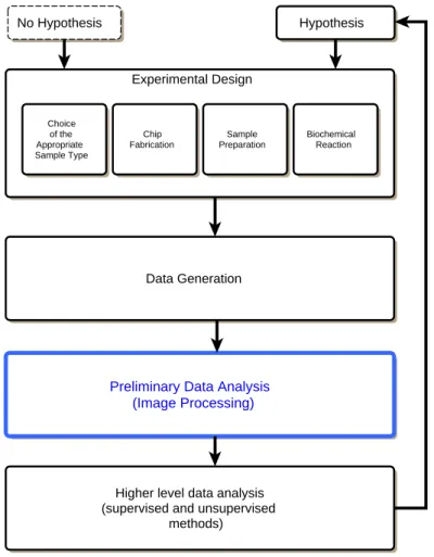
Figure 2.8: An overview of a microarray experiment and data analysis. After designing the experiment, the data should be acquired. These data must undergo a preliminary analysis basically by image processing step and quality assessment. The higher level analysis may involve various methods in order to carry out normalization and clustering. Usually, these analyses are relevant to the biological samples, the information required and the original hypothesis to be tested.
A microarray experiment generally consists of four distinct steps, see Figure 2.8. They are, 1) the design of the experiment which includes the choice of the appropriate sample type, chip fabrication, sample preparation and biochemical reaction; 2) data generation; 3) image processing; and 4) high level data analysis [Schena, 2000; Yang et al., 2002].
Chapter 2. 22 Background
2.4.2
Experiment Design
2.4.2.1 Choice of Sample Type
The first decision the researcher has to make when they design a specific experiment is to determine the type of the immobilized probes and the type of the sample. Since the gene expression profile is the most common application for microarray, cDNA is the most appropriate type while oligonucleotides is accounted as a second choice [Debouck & Good-fellow, 1999; Guo et al., 1994; Leung & Cavalieri, 2003; Li et al., 2004; Nuwaysir et al., 2002]. On the other hand, when the target of the study is genes that share a large sequence identity such as genes that belong to the same family, oligonucleotides are a better choice because of their fine ability to distinguish between similar sequences [Baggerlyet al., 2004]. However, other probe types such as proteins and antibodies are becoming popular as re-searchers start realizing the potential applications of the microarray technology, which will allow proteome-wide screening of protein function in parallel [Gl¨okler & Angenendt, 2003; Lueking et al., 1999].
2.4.2.2 Chip Fabrication
To produce a microarray, pre-synthesized probes, usually PCR products, are immobilized on the array slide at a pre-defined grid location. The product of this approach is usually called “spotted microarray”. Another method to produce the microarray is by using in situ, where each probe is individually synthesized on the surface of the slide [Debouck & Goodfellow, 1999; Yang et al., 2002]. The product of this approach is usually called “Oligonucleotide microarray”.
Common PCR primers can be used for the amplification of random sequences, which is very useful when there is no knowledge about the genome of the organism under study. Furthermore, microarrays can be used to perform a massive parallel sequencing [Diamandis, 2000; Zhouet al., 2006]. For this purpose, the target to be sequenced is immobilized, then a very large set of short and labeled probes has to be hybridized with this target. Then, the examination of the pattern of hybridization and the computation of the original DNA sequence have to be done [Drmanac et al., 1998]. Either that, or one should immobilize a very large set of short probes on a substrate and then hybridize these short probes with the labeled target of interest. Finally, biologists can infer the DNA sequence of interest by the analysis of the results [Pease et al., 1994].
Other materials that can be used as probes are Oligonucleotides, which are prepared by conventional phosphoramidite pre-synthesis [Pon & Yu, 2005]. By following this ap-proach, these oligonucleotides with their small size can minimize cross-hybridization that
Chapter 2. 23 Background
can possibly occur between distinct nucleic acids with sharing homology, from the same family. Given the existence of genes that share large sequence similarities in the genomes under study, oligonucleotides are often used in order to identify unique genes with greater specificity.
In the oligonucleotide microarray, in situ synthesis is merely a sequential addition of separate single nucleotides to a linker molecule directly onto the grid. This addition results in the synthesis of oligonucleotides, mostly with 20 nucleotides long.
Figure 2.9: Nylon-slide Microarray.
I) Substrate: The substrates that might be used for sample spotting can be of vari-ous types such as glass (Figure2.1), nylon membranes (Figure 2.9) or silicon chips (Figure
2.10). However, the glass slides are the most common ones because of their low cost, avail-ability, resistant to high temperatures, low fluorescence and generally favorable chemical characteristics [Cheung et al., 1999; Guo et al., 1994; Moore et al., 2002]
The attachment of the probes to the slide surface is based on the binding property of some chemicals. Generally, two substances are used to achieve this goal. The first material is the amine rich chemicals that give positive charges to the chip and interacts with the negatively charged probes. The second one is aldehyde chemistry where the 5’ primer, which is used for generation of probes through PCR amplification of the desired sequence, carries an aliphatic-amine group which attaches it to the aldehyde coated slide [Lemieux
et al., 1998].
II) Types of microarray chips fabrication technologies: Three main types of advanced technologies are commonly used to prepare the microarray slide: in situ, me-chanical spotting and the so-called ink-jet approach [Xiang & Chen, 2000; Yang et al., 2002]. Each one has some advantages and some disadvantages. Thus, researchers have to
Chapter 2. 24 Background
choose the most suitable one of these technologies based on their own needs.
* In Situ: In this method, oligonucleotides are built up base by base on the surface of the slide. The binding mechanism is based on the aldehyde chemistry. Usually, each nucleotide added to the oligonucleotide on the glass has a protective group to prevent the addition of more than one base at a time. The oligonucleotides in selected areas will be de-protected using chemicals or light in order to be ready before the next round of synthesis. This technology is very precise and highly automated since it allows direct fabrication of the chip using a sequence database without the need to add DNA clones, PCR products or other materials. Therefore, the risk of human error will be minimized.
Three main technologies are used for the de-protection in ”in-situ” synthesized array. Two are based on Photolithography, and the other is based on chemical de-protection:
1) Photodeprotection using masks: this is the basis of Affymetrixr technology [Brown & Botstein, 1999; Southern & Mir, 1999]. In this technology, specific masks are used in order to allow light to pass to some areas on the array but not to others. Each step of synthesis requires a different mask, and each mask is expensive to produce. This property makes this method expensive and time-consuming, and therefore limits the wider labora-tory usage of photolithography. In fact, in situ synthesized microarray chips are currently produced only in commercial settings [Guoet al., 1994]. However, once a mask set has been designed and made, it is straightforward to produce a large number of identical arrays.
2) Photodeprotection without masks: this method has been used by Nimblegen and Febit [Nuwaysir et al., 2002]. In this method, the light is directed via micro-mirror arrays to affect the specific area which is needed to be de-protected, instead of using masks.
3)Chemical protection with synthesis via inkjet technology: in this method, the de-protection is based on a chemistry similar to the standard DNA synthesizer. The printing device works in a similar method to the conventional color printers but with the 4 DNA bases instead of the color [Allain et al., 2001; Gershon, 2002; Singh-Gasson et al., 1999]. Because of its flexibility, this technology has been adapted to produce microarrays with cDNA probes [Epstein et al., 2002] in addition to oligonucleotides microarrays [Blanchard
et al., 1996].
* Spotted microarray: In this methodology, a robotic spotting device deposits the pre-made probes on a specific location on the surface of the chip. In order to accomplish the printing task, the spotting robot contains a set of pins, which need to come close enough to the substrate to spot the probes. Those pins have to reload new samples after each deposit from a microtiter well plates.
Besides the low density of this type of microarrays, the high risk of the wrong ma-nipulation of the pre-made probes is its main drawback. However, the low cost of the
Chapter 2. 25 Background
method makes it suitable for a wider range of laboratories, with limited budgets, and it is probably the predominantly used method for microarray chips’ fabrication in the academic community.
* Ink jets: In a way it is similar to the spotted array methodology. The probes should be pre-prepared and then loaded into the miniature nozzle, which is controlled by a robotic system to ensure that the printing is at specific co-ordinates of all spots. After the printing of each spot, the nozzle is washed and loaded with the next sample of interest. One of the advantages of this technology is the un-necessity of the physical contact between the nozzle and the slide surface.
Figure 2.10: Oligonucleotides Microarray.
2.4.2.3 Target Preparation and Labeling
Many biological methods have been developed in order to prepare and label samples for microarray experiments. Basically, these methods depend on the biological query and the type of probes used in the experiment. Generally, the first step is to extract mRNA forming the cells or tissues of interest. These extracted mRNA will be used to synthesize cDNA. Most laboratories use fluorescent labeling with dyes of choice, usually Cyanine-3 (Cy3, green) and Cyanine-5 (Cy5, red). In the most common experiments, two samples
are hybridized to the arrays. Molecules derived from the reference sample are labeled with one type of dye, say Cy3, while the nucleic acid derived from the examined sample are
labeled with a second type of dye, sayCy5, and then the samples are mixed together. This
allows the simultaneous measurement of both samples. When the resulted chip is scanned, up-regulated genes appear red (because of the high ratio Cy5/Cy3) while down-regulated
genes appear green. Therefore, genes whose expression levels have not been affected appear yellow, as the red and green dyes are present in equal amounts.
Chapter 2. 26 Background
There are generally three labeling approaches. The first is direct incorporation by reverse transcriptase; the fluorescent tags are immediately attached to the sample nucleic acid in a covalent manner. The second method is indirect labeling that also uses a reverse transcription reaction; a second molecule, commonly biotin, serves as an intermediate between the fluorescent tag and the probe. The third and the least common method for labeling is by random primed labeling using the Klenow fragment of DNA polymerase I. Many approaches have been developed to reduce the sufficient amount of RNA, which is required for an experiment to get a better quality labeling and, therefore, to improve the sensitivity of the detection process [Baggerlyet al., 2004].
2.4.2.4 Biochemical Reaction (Hybridization)
When the mixture of labeled samples (reference and testing) is ready, the next step is to expose the slide with the specified probes to these resulted materials. Biological bonding, which is called hybridization, is the stage in which the probes on the slide and the labeled samples form heteroduplexes bind together. Hybridization is a very complex mechanism, which is affected by many factors. The non-porous slides would increase the chance of two complementary molecules to come in physical contact in a certain amount of time. Furthermore, this type of substrate reduces the amount of samples needed for the experi-ment. In addition to the slide substrate properties, these conditions include temperature, humidity, salt concentrations, formamide concentration, volume of target solution and op-erator. The hybridization could be performed manually or, alternatively, robotic-ally by a hybridization station.
For instance, with the reference sample labeled with Cy3 (green) and the tested sample
labeled with Cy5 (red), the exposure of the chip to the mixture of both labeled samples will cause hybridization. The amount of red and green dyes present at any specific spot (corresponding to a particular gene) will depend on the way by which the applied treatment affects the expression level of this specific gene in the tested tissue [Brazma et al., 2000].
For the genes that are not affected by the treatment, the amount of the corresponding mRNA is the same in both samples. Therefore, the red and green labeled molecules are of equal abundance and will present equal amount at these genes’ assigned spots; the reflected color will be yellow. Besides, the genes that are over-expressed in the tested tissue would lead to a mixture which contains more red-labeled molecules representing those particular genes. Furthermore, the genes that are under-expressed in the tested tissue would produce a mixture with more green labeled molecules [Sherlock & Hernandez-Boussard, 2001].
Chapter 2. 27 Background
to: 1) remove any excess hybridization solution from the array and ensure that the only labeled molecules on the array are the molecules that have specifically bound to the features on the array. 2) increase the stringency of the experiment by reducing cross-hybridization. After washing, the slide will be ready to be scanned.
2.4.3
Image Acquisition and Data Readout
At the end of the laboratory process, the image of the surface of the hybridized chip should be acquired. The heteroduplexes on the slide, where the target has hybridized to the probe, contain dye that fluoresces when excited by light of an appropriate wavelength. These dyes allow us to detect the amount of targets bound to each spot using several technologies. The most common one is the high resolution confocal laser scanners. The scanner contains one or more lasers that are focused onto the array; most scanners for two-color arrays use two lasers.
The software integrated with every scanner type extracts intensity signals from the chip and converts them into a numerical value; i.e., monochrome image. With the two-channel microarray, the output of the scanner is usually two monochrome images: one for each of the two lasers in the scanner. These images are combined to create the red (green) color images of microarrays. The images are usually stored as 16 bits Tagged Image File Format (TIFF) [Schermer, 1999]. This means that the intensity of each pixel in each channel is quantified as a 16-bit number, which takes values between 0 and 65535. Usually, background is approximately 100 and saturation can occur when the average pixel intensity is larger than 50,000. The microarray can detect intensities over