DISCUSSION PAPER SERIES
Forschungsinstitut zur Zukunft der Arbeit Institute for the Study of Labor
Gender Differences in Competition
Emerge Early in Life
IZA DP No. 5015
June 2010 Matthias Sutter Daniela Rützler
Gender Differences in Competition
Emerge Early in Life
Matthias Sutter
University of Innsbruck University of Gothenburg and IZA
Daniela Rützler
University of Innsbruck
Discussion Paper No. 5015 June 2010 IZA P.O. Box 7240 53072 Bonn Germany Phone: +49-228-3894-0 Fax: +49-228-3894-180 E-mail: iza@iza.org
Any opinions expressed here are those of the author(s) and not those of IZA. Research published in
this series may include views on policy, but the institute itself takes no institutional policy positions. The Institute for the Study of Labor (IZA) in Bonn is a local and virtual international research center and a place of communication between science, politics and business. IZA is an independent nonprofit organization supported by Deutsche Post Foundation. The center is associated with the University of Bonn and offers a stimulating research environment through its international network, workshops and conferences, data service, project support, research visits and doctoral program. IZA engages in (i) original and internationally competitive research in all fields of labor economics, (ii) development of
IZA Discussion Paper No. 5015 June 2010
ABSTRACT
Gender Differences in Competition Emerge Early in Life
*We study gender differences in the willingness to compete in a large-scale experiment with 1,035 children and teenagers, aged three to eighteen years. Using an easy math task for children older than eight years and a running task for the younger ones we find that boys are much more likely to enter a tournament than girls across the whole age spectrum considered here. This gender gap is observed already with three-year olds, indicating that gender differences in competitiveness emerge very early in life. The gap is robust to controlling for gender differences in risk attitudes and overconfidence.
JEL Classification: C91, D03
Keywords: competition, gender gap, experiment, children, teenagers
Corresponding author: Matthias Sutter
Department of Public Finance University of Innsbruck Universitaetsstrasse 15 A-6020 Innsbruck Austria E-mail: matthias.sutter@uibk.ac.at *
We would like to thank Loukas Balafoutas, Gary Charness, Uri Gneezy, Magnus Johannesson, Martin Kocher, John List, Pedro Rey-Biel, Daniel Schunk and seminar participants at the University of Arizona in Tucson, University of California at Santa Barbara, University of Erfurt, University of Gothenburg, Stockholm School of Economics, Max Planck Institute of Economics in Jena and Economic Science Association European Meeting in Innsbruck for helpful comments. Financial support from the Austrian National Bank (Jubilaeumsfondsprojekt 12588) and the University of Innsbruck is gratefully acknowledged. We are particularly grateful to Thomas Plankensteiner from the Central School Administration Board of Tyrol, Michaela Hutz, Barbara Raithmayr and Martina Zabernig from the Board of Tyrolean Kindergartens, and the headmasters of the involved schools and Kindergartens, Hildegard Flöck, Max Gnigler, Siegmund Heel, Gottfried Heiss, Eva Nora Hosp, Ulrike Künstle, Hermann Lergetporer, Claudia Pertl, Bernhard Schretter, Peter-Paul Steinringer and Birgit
1
Introduction
In order to be successful on labor markets with respect to getting more attractive and better paid jobs it is not only important to acquire human and social capital, but it is also essential to feel comfortable in competitive environments and accept the challenge of competition instead of shying away from it. Recent research has documented strong differences between men and women as far as the willingness to compete and the performance in competitive situations is concerned. Many studies have shown that men often react more strongly to competitive pressure than women, and that women are more likely to shy away from competition, even when they are equally qualified (e.g., Gneezy, Niederle and Rustichini, 2003; Gneezy and Rustichini, 2004; Datta Gupta, Poulsen and Villeval, 2005; Niederle and Vesterlund, 2007, 2010; Booth and Nolen, 2009; Croson and Gneezy, 2009; Gneezy, Leonard and List, 2009; Cason, Masters and Sheremeta, 2010; Dohmen and Falk, 2010; Niederle, Segal and Vesterlund, 2010; Wozniak, Harbaugh and Mayr, 2010). These gender differences in competitiveness may at least partly contribute to the persistent gender gap in wages and top-level positions on the labor market (see, for instance, Altonji and Blank, 1999; Blau and Kahn, 2000; Bertrand and Hallock, 2001; Weichselbaumer and Winter-Ebmer, 2007; Blau, Ferber and Winkler, 2010).
Hence, in order to deal with differences in competitiveness as one source for gender gaps on the labor market it is important to examine where these differences come from and how they might evolve over time. Recent work – that will be discussed in more detail below – provides first evidence on the influence of culture (Gneezy et al., 2009), social learning (Booth and Nolen, 2009) or hormones (Wozniak et al., 2010). No study has investigated gender differences in competitiveness from early childhood to the late teenage years, though. Nothing is known so far as to whether the gender gap in competitiveness emerges relatively early or late in the course of life. Gaining knowledge about the periods in life in which a gender gap in competitiveness exists is a precondition, however, to tailor the timing and type of suitable policy interventions to narrow down or even close this gap, with the aim of providing women with better chances on labor markets later on in life.
running) task under a competitive or non-competitive payment scheme. We find already in our youngest age group of three-year old children that boys are significantly more likely than girls to choose the competitive scheme. In fact, this gender gap persists in all age groups covered in our sample, and it is robust to controlling for gender differences in risk attitudes and overconfidence. This main result indicates that the gender gap in competitiveness exists already very early in life, and does not change notably after the age of three years. Given the young age of three years from which on we find persistent gender differences, our findings are consistent both with an explanation that favors the impact of nurture – in the form of infants’ education as well as social and cultural learning – and an explanation that draws on the power of nature – in the form of biological factors. Recent papers have found support both for nature and nurture in studies with adults.
Gneezy et al. (2009) have shown that gender differences in competitive behavior and the willingness to compete are strongly affected by cultural conditions. They conducted experiments with adult members of a patriarchal tribe in Tanzania and a matrilineal tribe in India. In the matrilineal tribe of the Khasi, the youngest daughter in a household is always heir to the parents’ fortune and, in practice, the husband always moves into the wife’s household. The Gneezy et al. (2009) experiment consisted of a single stage, where subjects had to toss tennis balls into a bucket. Before performing the task subjects had to choose one of two possible payment schemes, either a piece rate per successful shot or a tournament scheme with higher incentives, but the possibility of earning nothing in case of losing the tournament. Subjects were not informed about their competitor’s identity and gender. Gneezy et al. (2009) found that in the matrilineal culture more women than men chose the tournament, while in the patriarchal culture more men than women chose the competitive payment scheme (similar to what is known from experiments in highly industrialized states; see, e.g., Niederle and Vesterlund, 2007). While these results do not rule out the possibility that nature (such as genetic predispositions and physiological factors) have a strong impact on gender differences in competition, they show that the social framework prevalent in a specific culture plays an important role for the behavior of adults in competitive environments.
The first contribution on the influence of biological factors on the gender gap in competition is a very recent paper by Wozniak et al. (2010). They investigate biological explanations for the observed gender differences by examining how (adult) women’s competitive choices change with hormonal fluctuations. While Wozniak et al. (2010) can
replicate the finding that men are more likely to choose competitive compensation schemes1, they also find that hormonal fluctuations during the menstrual cycle have a significant impact on the choices of women. During their low-hormone phase women are less likely to enter competitive environments than women in a non-low-hormone phase of the menstrual cycle. This shows that biological factors can influence the size of the gender gap in the willingness to compete.
Compared to both Gneezy et al. (2009) and Wozniak et al. (2010) our paper is different through its use of a subject pool of children and teenagers who are three to eighteen years old. Despite this fact, our paper should be considered as complementary to their approaches. In the life-span from three to eighteen years important social and biological changes take place (see, e.g., Kail and Cavanaugh, 2010). Children have to enter the (public) education system and get exposed to socialization and social learning from outside of the own family. The body changes rapidly and faces many biological and cognitive challenges (such as puberty) in the transition to adolescence and adulthood. We are interested in whether we can detect changes in the behavior of boys and girls in competitive environments in this important period of life, in particular whether the gender gap reported for adults is persistent also in young children and teenagers.
Of course, we are not the first ones to present an experiment on the behavior of children and teenagers in competition. Gneezy and Rustichini (2004) have shown for a sample of 240 nine- to ten-year old Israeli children that boys increase their performance in a 40 meters sprint more when competing against another child – instead of running alone – than girls do. Recently, Dreber, von Essen and Ranehill (2010) have not been able to replicate this gender difference in response to competition (in running, skipping rope or dancing) in a sample of 438 eight- to ten-year old Swedish children. Dreber et al. (2010) argue that one reason for the lack of a gender difference might be the very egalitarian treatment of men and women in the Swedish society, lending support to the general finding in Gneezy et al. (2009) that culture (and thus social norms) are important for the size and direction of the gender gap in competition. Whereas Gneezy and Rustichini (2004) and Dreber et al. (2010) have studied how girls and boys change their behavior when they are actually exposed to competition, a previous step in this process is whether girls and boys are equally likely to enter competition.
Booth and Nolen (2009) have examined this issue by letting 260 fifteen-year old British teenagers choose whether they want to be paid in a maze-solving task according to a tournament or piece rate scheme. The twist in their study is that these children attended either a single-sex or coeducational school. In general, Booth and Nolen (2009) replicate a gender gap in competition entry decisions by observing that girls choose the tournament scheme less often than boys (except when girls compete only against other girls). However, they report a behavioral difference between girls from coeducational schools and from single-sex schools. Girls from single-sex schools are more likely to enter competition than coeducational girls. Although there are subtle issues of self-selection (of different types of girls into different school types) that make this latter result vulnerable to criticism (see, e.g., Niederle and Vesterlund, 2010), the results of Booth and Nolen seem to support the conclusion that social learning is important.
Compared to these earlier studies that have run experiments with children, our paper is the first one to cover an age range of fifteen years from early childhood to the late teenage years, while earlier studies have had at most two years of age difference in their sample. Our sample is also at least twice as large as the samples used in previous studies, thus increasing the validity of results. Most importantly, no previous study has examined the behavior of children younger than eight years old, although the main development of a human subject’s character traits – that might well include one’s attitude towards competition – takes place in the first few years of life (Kail and Cavanaugh, 2010). Hence, it seems particularly important to examine the existence of a gender gap in young children’s willingness to compete.
The rest of the paper is structured as follows. In Section 2 we explain the experimental design of the math task that was used for nine- to eighteen-year old children and teenagers. The results for this task are presented in Section 3. In Section 4 we introduce the design and procedure of the running task for our three- to eight-year old participants. Since competing in math tasks is not feasible for the youngest participants, we chose running as a more natural and familiar task for this second experiment. The results for the running task are reported in Section 5. Section 6 discusses our overall findings from both experiments and concludes the paper.
2
Design of Experiment I: Competition in a Math Task (9- to 18-Year
Old Children)
The experimental design of our first experiment builds on Niederle and Vesterlund (2007). Like them we used a simple math task of adding up two-digit numbers as the experimental task. The reason for choosing a math task was not only that we follow the literature (Niederle and Vesterlund, 2007) to make comparisons to earlier studies with adults easier, but also because math test scores serve as a good predictor of future income (see, e.g., Murnane et al., 2000; Weinberger, 2001). Moreover, there are typically no gender differences
in such easy math tasks (Hyde et al., 2008), making it a priori less likely to find gender
differences in the willingness to compete.
At the beginning of the experiment, subjects were randomly assigned to groups of four
persons. The group assignment was fixed for all four stages of the experiment.2 Each stage
was only explained after the previous one had been finished. The instructions were explained verbally, following a fixed written script (see Appendix A1). Questions were answered privately. Participants had to perform the task by entering their solutions on a keyboard (using zTree; Fischbacher, 2007). Hence, before the experiment started, all participants were given enough time to acquaint themselves with the keyboard and the mouse, and before Stage 1 there was also a one-minute training sequence. There was no feedback (concerning the tournament outcome) given until the very end of the experiment in order to avoid past experiences influencing future choices. At the end of each stage participants were only informed about the number of calculations they had worked on and how many of them had been correct. The sequence of stages was as follows:
Stage 1 – Piece rate: Each participant received €0.50 for each calculation that was
correctly solved within the limit of two minutes.3 There was no competition involved in this
stage.
Stage 2 – Tournament: Here participants had to compete in the same task against the three other group members. The group member who solved the most calculations correctly in Stage 2 was paid €2.00 for each of them. The other three group members received nothing. Ties were broken randomly (also in the subsequent stages).
Stage 3 – Choice of compensation scheme for future performance: Every group member could choose whether (s)he wanted to solve the calculations under a piece rate scheme (as in Stage 1, receiving €0.50 per correct solution) or a tournament scheme (as in Stage 2). If the tournament was chosen, then a subject’s performance in Stage 3 was
compared to the other group members’ performance in Stage 2.4 Winners received again
€2.00 per correct solution, losers nothing.
Stage 4 – Choice of compensation scheme for past performance: Subjects did not have to perform the math task in this stage, but had to choose between a piece rate and tournament scheme for their past performance in Stage 1. The piece rate scheme paid €0.50 per correct solution that was achieved in Stage 1. The tournament scheme paid €2.00 per correct solution if a subject’s Stage 1 performance was the best in his/her group. Otherwise he/she received nothing. This stage is a control condition that allows us to investigate whether the gender gap in tournament entrance persists even when no real performance is required.
Elicitation of expected ranks: After the completion of Stage 4 participants were asked about their expected rank in their group of four members both for their performance in Stage 1 and in Stage 2. An expectation of rank 1 would indicate that a participant expected to be the best performer in his/her group in a particular stage. Each correct expectation was paid €0.50. Note that the question on expectations was only introduced at the very end. Hence, hedging (for instance by performing particularly poorly in Stage 2 in order to win for sure €0.50 by expecting rank 4 for this stage) was not possible.
At the end of the experiment one stage was randomly selected for payment by letting one student draw one of four numbered cards. By paying only one stage we wanted to avoid income effects. The expectations were paid in any case. In addition to their performance-related payoff each participant received a show-up fee of €1.00. The overall payoff was distributed several days after the experiment by a school’s secretary (who was not involved in the experiment) in sealed envelopes marked with a six digit code only known to students in order to preserve anonymity.
The experiment was run in three elementary and four grammar schools in Innsbruck, Schwaz and Völs, three close-by cities in the federal state of Tyrol in the Western part of
4
Using the other group members’ past performance has several advantages. First, tournament entry decisions do not depend on a subject’s expectation about the other members’ entry decisions, but only on the subject’s beliefs about her/his own ability and the ability of the other group members in Stage 2. Second, Stage 2 performances are competitive performances, and thus a subject competes against others when they were also exposed to a competitive payment scheme. Third, entering competition does not impose externalities on others. In principle, this means that Stage 3 is an individual decision making problem. Note that this scheme also implies that it is possible that all group members entering the competition in Stage 3 may win or all lose since they are competing against the others’ performance in Stage 2.
Austria. Sessions were conducted between January and March 2009. This experiment was part of a larger project with a series of experiments in which we visited the involved schools several times in a period of two years, exposing children to different experimental tasks (in order to study, e.g., their social preferences – see Sutter et al., 2010a – or their risk and time preferences – see Sutter et al., 2010b). The whole project was approved by the central school administration board of Tyrol and the headmasters of the selected schools. All parents of involved children and teenagers were informed in a letter about the project and its aim to study economic decision making of children, without revealing any specific details or experimental tasks, though. Parents were given the option to opt out their child from the project, and five out of more than 700 did so. All other parents consented. Children and teenagers were also instructed that participation was completely voluntary. Since they were told that they could earn some money in the experiments, no single student refused to participate in any of the experiments.
Table 1 about here
In total, we had 717 participants from 37 different classes from 5 different grades
(grades 4, 6, 8, 10, and 12). The youngest participants were nine to ten years old (4th grade),
and the oldest ones seventeen to eighteen years (12th grade). We used a between-subjects
design with two treatments. In the MIXED treatment they were told that each group of four members would have exactly two boys and two girls. In the SINGLE-SEX treatment they were told that each group consisted of four members of their own gender. Within a given class, all students faced the same treatment. In both treatments students were informed that their other three group members would be randomly drawn from the pool of students in any of the participating schools who were in the same grade as they were in. Table 1 summarizes the distribution of participants by age, gender and treatment. Overall, an experimental session lasted about 50 minutes, and participants earned on average €6.58 (including the €1 show-up fee).
3
Results of Experiment I (9- to 18-Year Old Children)
3.1
Performance and Expected Ranks in Stages 1 and 2
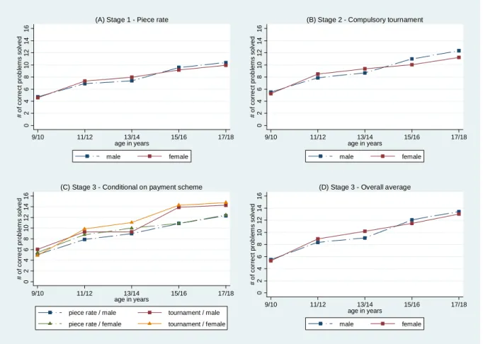
Panels (A) and (B) of Figure 1 show the average performance of boys and girls in Stage 1 (piece rate) and Stage 2 (compulsory tournament). Generally we see an almost linear increase in the number of problems solved correctly with age. As expected, participants get more efficient in adding two-digit numbers when they get older. Comparing panels (A) and (B) also reveals that the average performance is higher under the tournament scheme (Stage
2) than the piece rate (Stage 1), and the increase in performance is significant (p < 0.02 for
each gender within each age group; Wilcoxon signed rank tests). The increase from Stage 1 to Stage 2 is perhaps not only due to the higher incentives under the tournament scheme, but also to some learning going on.
Figure 1 and Table 2 about here
Panels (A) and (B) of Figure 1 reveal that there are only very small differences between girls and boys. In Table 2 we present OLS-regressions with the number of correct answers in Stage 1 (models 1a and 1b) and in Stage 2 (models 2a and 2b) as dependent
variables.5 We see from Table 2 that there are no significant differences in the performance of
girls and boys, neither in Stage 1 nor in Stage 2, even when accounting for the treatment
(dummy for the Single-Sex treatment) and an interaction term of Single-Sex and Female.
Running a series of Mann-Whitney U-tests shows that there are also no significant gender differences concerning the quality of effort, measured as the relative frequency of correct
answers in each stage of the experiment.6 On average, the relative frequency of correct
answers is 87%.7 Hence, differences in the ability to perform in the math task can be ruled out
to explain possible gender differences in the willingness to choose the tournament in Stage 3.
Figure 2 about here
5
We have also run all models in Table 2 as Poisson regressions in order to account for the fact that the dependent variable can only have integer values. All main results stay the same. The same holds true also for Table 4 below.
6
There is a single exception for Stage 2 in the group of thirteen-/fourteen-year olds, where males have a significantly higher frequency of correct answers.
7
We have also checked whether the increase in performance from Stage 1 to Stage 2 differs across gender (as the results of Gneezy and Rustichini, 2004, for a running task might suggest). However, we find no gender differences in the increase of performance either, nor do we find any influence of age or treatment on the change in performance across the first two stages (see the regressions in Table B.1 in Appendix B).
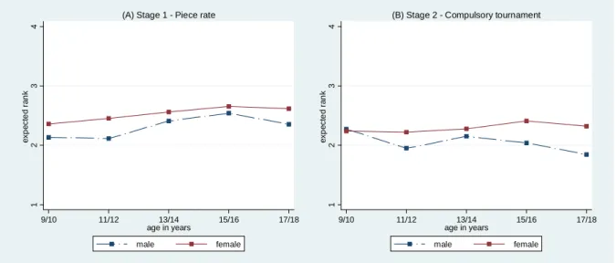
Recall that at the end of this experiment we asked subjects about their expected ranks in Stages 1 and 2. A rank of 1 indicates an expectation to be the best performer in the group, while a rank of 4 means to be the worst one. Figure 2 shows the average expectations of girls and boys in each age group. Except for a single case, girls have on average more pessimistic expectations than boys, both in the non-competitive Stage 1 and the competitive Stage 2.
Of course, if subjects had well-calibrated expectations, then the average expected rank would have to be 2.5. However, Figure 2 reveals that subjects are on average overconfident and boys are even more so than girls. The gender difference in overconfidence is clearly confirmed in ordered probit regressions (shown in Appendix B, Tables B.2 and B.3). Both for the expected rank in Stage 1 and in Stage 2 we find that girls’ estimated expectation is on average roughly 0.4 ranks worse than that of boys. This significant effect is robust to controlling for the actual performance (that did not differ between girls and boys) and age (with younger children being more overconfident).
3.2
Entry into the Tournament and Subsequent Performance
Figure 3 shows the entry rates of girls and boys into the tournament payment scheme in Stage 3 of the experiment. Although performance in Stages 1 and 2 was practically identical, the gender differences in tournament entry are striking. Across all age groups, 19% of girls, but 40% of boys, choose to enter the tournament (p < 0.001; χ²-test).
Figure 3 and Table 3 about here
Table 3 reports the results of a series of probit regressions where the dependent variable is coded 1 if a subject chooses to enter the competition in Stage 3, and 0 otherwise. The baseline specification controls for gender and age effects (1a) as well as treatment effects
by including a dummy for the single-sex treatment (Single-Sex) and an interaction term of
gender and treatment (Single-Sex*female) (1b). We find a strong gender effect, with a roughly
treatment and gender do not have a significant effect, though.8 Age seems to have some
influence, but often insignificantly, as becomes also clear from the following regressions.9
Specifications (2a) and (2b) add as further controls a subject’s actual performance in
Stage 2 (Correct 2) and the absolute increase in performance from Stage 1 to Stage 2 (Correct
2 – Correct 1). The latter shall capture a subject’s potential of increasing performance under competition. Not surprisingly, the actual performance has a positive impact on tournament entry. For each additional problem solved the likelihood of entering the tournament increases by roughly three percentage points. The increase in performance from Stage 1 to Stage 2 has no predictive power. The gender gap, however, remains significant and of equal size even after the inclusion of these additional controls.
In specifications (3a) and (3b) we also consider the expected rank for Stage 2 as explanatory variable, as this shall capture a subject’s expected relative performance under a competitive payment scheme. Since in the tournament it’s only crucial to win (or expect to
win), we include a dummy for an expected rank of 1 (Rank 2 = 1) in order to see how an
expectation to win affects behavior. We see that subjects who expect to win are about 33 percentage points more likely to enter the tournament. The number of correct answers in Stage 2 is still significantly positive, and, most importantly, the gender gap persists even after controlling for expectations. Recall from the previous subsection that there are significant gender differences in the expected rank. Including the expectation to win reduces the marginal
effect of the Female-dummy slightly by about four percentage points. Hence, different
expectations can explain some part of the observed gender gap, but a substantial gap remains.
In the final specifications (4a) and (4b) we add a subject’s math grade (Math) and
his/her risk preference (Risk aversion) as independent variables. In the Austrian school system
grades range from 1 (best) to 5 (worst). The risk preferences of subjects were determined in a different experiment (about six to ten months earlier) by letting them choose between a lottery and an increasing sure amount of money. From that we have constructed a variable that
ranges from zero (strong risk loving) to one (strong risk aversion).10 The results in columns
(4a) and (4b) show that risk-averse subjects are significantly less likely to enter the
8
We have also run all regressions reported in Table 3 with an additional dummy for one girls-only school that is included in our sample. The dummy is never significantly different from zero, and its inclusion does not change our main results.
9
Including a quadratic age term in the various specifications to capture the U-shape in Figure 3 does not change our main results either.
10 More precisely, the lottery yielded a prize π > 0 or zero with a 50:50 chance and children had to indicate in a
choice list whether they preferred the lottery or a safe amount that increased from π/20 to π in 20 steps of width π/20. From this we determined the interval including the certainty equivalent, took the midpoint of this interval and then calculated our measure of risk aversion as 1 – (certainty equivalent/prize π). See Sutter et al. (2010b) for more details.
tournament, and that subjects with better (i.e., lower) math grades are more likely to enter it. Most importantly, though, adding these further controls does not change our main result of a
persistent and significant gender gap in the likelihood to enter the tournament.11
After having analyzed the decision to enter the tournament in Stage 3 we have a brief look at the performance in Stage 3. Panels (C) and (D) of Figure 1 show the average performance in Stage 3, once conditional on entering the tournament, and once overall. In general, those who enter the tournament have a better performance than those who don’t. This becomes also clear in columns (2a) and (2b) of Table 4 in which we regress the number of correct answers in Stage 3 on age, gender, treatment, and the decision to enter the tournament (Tournament 3). Those who choose the tournament solve about 1.5 problems more than those opting for the piece rate. Again we see an increase in performance with age, and it is noteworthy that in Stage 3 we even find significantly better performance for girls.
Table 4 and Figure 4 about here
Finally, we show in Figure 4 the decision in Stage 4 of the experiment. In this stage subjects had to decide whether to submit their performance in Stage 1 to a piece rate scheme or a tournament (against the other three team members). Figure 4 shows the relative frequency of choosing the tournament. Again, we see that boys enter the tournament much more often than girls, which largely replicates the findings of Stage 3. Thus we find female antipathy toward competitive environments not only in situations where subjects have to compete subsequently (as in Stage 3), but also when subjects have to decide on whether to compare
their own past performance to someone else’s (as in Stage 4).12
As an intermediate summary of our first experiment we conclude that the gender gap in the willingness to enter competition in a tournament prevails already by the age of nine years and persists throughout the teenage-years. Given this persistent gap already at this young age we devised an experiment that could be run with even younger children to examine whether the gap would persist even at a younger age.
11
4
Design of Experiment II: Competition in a Running Task (3- to
8-Year Old Children)
The second experiment modifies the original design of Gneezy and Rustichini (2004). We let children aged three to eight years run a distance of 30 meters in their Kindergarten’s or school’s gym. Research has shown that there are no systematic gender differences in short sprints at the age level of our participants (see, e.g., Papaiakovou et al., 2009). Hence, like our
math task, this task does not imply an a priori advantage of boys over girls with respect to
objective performance.
The experiment consisted of two stages, with an intermediate elicitation of expectations. In both stages participants could earn points depending on their performance. After the experiment, these points could be exchanged for small presents, such as sweets, stickers, balloons, or pencils. These presents were shown to the children at the beginning of the experiment. Each item “cost” one point in the experiment, and we chose the items such
that they were roughly of equal monetary value.13 The two stages of the experiment were as
follows:
Stage 1 – Running on your own: Children were asked to run 30 meters in their gym as fast as possible. Children received no feedback on their own time and their relative position to the other children in their cohort until the end of the experiment, but were told that all children who were relatively quick (all with a below-median runtime) would earn two points,
while the others (with an above-median runtime) would earn one point.14
Stage 2 – Choice of compensation scheme for future performance: In Stage 2 children could choose whether to repeat the running task by either running again on their own, or by competing against another child in their group (of same age). Children were told that in case of competition they would be matched with a child whose runtime in Stage 1 was approximately the same as his/her own and who also wanted to run against another child. The payment scheme was as follows: If running on his/her own, a child could earn two experimental points if his/her time was better than the median of Stage 1, and one point otherwise. In the competition, these points would be doubled for the winner, while the loser
13
Harbaugh, Krause and Berry (2001) study the rational choice behavior of children and teenagers and show that even young children make rational consumption choices. Hence, we can be confident that the children in our experiment can make rational choices in exchanging their points into goods.
14
In fact, although it’s an individual task in Stage 1, the reward depends also on others’ performance. Given that the groups of children were relatively large (15 to 20 children) it was next to impossible for children to know their relative standing exactly. We had considered using a fixed, and pre-announced, time instead of a median-split, but – after consulting with Kindergarten teachers – it became clear that children in Kindergarten have difficulties with the measurement of time in seconds, while they can perfectly understand to be relatively faster or slower. Hence, we opted for using a median-split.
would not earn any points. This means that a winner earned four points if his/her time was below the median of Stage 1, but two points otherwise.
Asking for expected ranks: After having explained the rules for Stage 2, but before performing the task, children were asked about their beliefs concerning their performance in Stage 1, i.e., whether they were in the relatively faster or slower group. We also asked them about their expectation for Stage 2, i.e., whether they expected to win the competition or not. Note that we also asked those children who opted out of the competition in Stage 2 about their (hypothetical) expectation whether or not they would have won the competition if they had had to compete against another child. This was done in order to keep the conditions identical
for all children. Note that in this experiment we asked about expectations before the actual
competition. Since the competition in a running task is immediately resolved and obvious for the involved children it was impossible to ask about their expectations on relative
performance after the fact. We did not pay any points for these expectations, though, in order
to avoid that someone can hedge by stating an expectation to lose and then run slowly to lose the competition and earn some points from a correct expectation.
The instructions for Stage 1 were carefully explained to all children in public, following a fixed script (see Appendix A2). The second stage was explained to each child individually and the experimenter checked for proper understanding of the task and the rules by letting each child repeat the rules. Only after repeating the rules the child had to make the decision about whether to run on his/her own or compete against another child and then state his/her expectations.
This experiment was run in three Kindergartens and two elementary schools in Innsbruck and Schwaz. Sessions were conducted in May and June 2009 and May 2010 and took place in the regular gym classes (lasting 100 minutes). Upon approval of the central school administration board of Tyrol and the headmasters of the respective institutions, parents were informed in a letter that some members of the local university would attend gym classes to measure athletic performance.
them are excluded from the following analysis because they were not able to correctly repeat the rules for Stage 2. This leaves us with data from 227 children in Kindergarten. In order to bridge the age gap to the youngest participants in our math task (nine- to ten-year olds in experiment I) we also ran the second experiment in the second grade of two elementary schools. We had 91 participants in these schools. None of them had problems in repeating the rules for Stage 2. Therefore, we have a total of 318 children from three to eight years for our analysis of the running task. Table 5 summarizes the number of girls and boys in the different cohorts.
5
Results of Experiment II (3- to 8-Year Old Children)
5.1
Actual and Expected Relative Performance
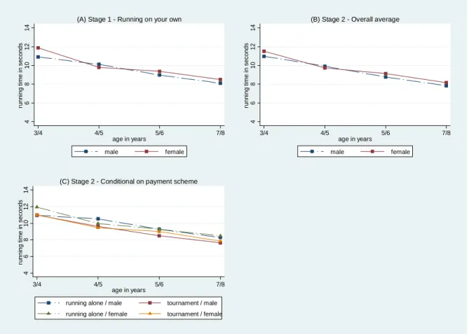
Figure 5 shows the average running times for girls and boys in the different age groups. In all panels of Figure 5 we note an almost linear increase in speed across the four age groups. In Stage 1, i.e. panel (A), girls are slightly slower than boys, in particular in the youngest age group of three- to four-year olds. Panel (C) provides the running times contingent on gender and a subject’s decision to enter competition or not. Those running against another child (see the straight lines) are always faster than those running on their own.
Figure 5 and Table 6 about here
These observations are confirmed in the OLS-regressions reported in Table 6. Column
(1) regresses the running time in Stage 1 on age and a gender dummy (Female). The
coefficient for age shows that getting one year older reduces the time by roughly 0.8 seconds. The gender dummy is significant, meaning that girls are slower. However, this effect is only driven by the youngest age group of three- to four-year olds. Adding a dummy for this group
would make Female insignificant. Columns (2) and (3) consider the running times in Stage 2.
When controlling for the decision to enter the tournament, gender is no longer significant.
Figure 6 about here
Before turning to the children’s decision whether or not to compete in Stage 2 we display in Figure 6 the average expectations about relative performance. Panel (A) shows the relative frequency with which children expect to be in the faster (instead of the slower) group in their session. We see a remarkable degree of overconfidence, with an average of 91% of
children in Kindergarten (age three to six) expecting to be in the faster group. While boys are on average slightly more overconfident, the gender difference is not significant (in a regression not reported here). Panel (B) of Figure 6 shows the relative frequency with which children expect to win the competition in Stage 2, conditional on whether subjects have actually chosen to compete (straight lines) or not (broken lines). The general pattern emerging from Panel (B) is that those who compete are clearly more confident to win.
5.2
Entering Competition in Stage 2
Despite the small differences in performance, we note from Figure 7 significant gender differences in the willingness to enter competition also in this experiment. Across all age groups, we find a difference of 15 percentage points in the relative frequency of boys and girls entering the competition (p < 0.01; χ²-test).
Figure 7 and Table 7 about here
Table 7 reports the results from several probit regressions that confirm the insights from Figure 7. The dependent variable is a child’s decision to compete against another child
in Stage 2. In column (1) we control for gender and age effects. The Female-dummy is
significantly negative, and girls are estimated to be roughly 15 percentage points less likely to compete. In column (2) we add the running time in Stage 1 as a control that takes into account physical ability in this task. As expected, slower children are less likely to compete (by about 6 percentage points). However, the gender gap remains significant and of similar size as in column (1). In column (3) we add children’s expectations as control. The expectation about winning has a strongly positive influence (raising the likelihood of entering by about 50
percentage points). The Female-dummy, however, is still significant.15
We conclude from our second experiment that the gender gap in the willingness to compete can already be found in three- to four-year old children in Kindergarten. From this age on the gender gap is persistent.
6
Conclusion
In this paper we have studied the competitive behavior of 1,035 children and teenagers, aged three to eighteen years. In particular, we have studied whether the willingness
to compete differs between boys and girls in the period of life covered in our sample.16 A
gender gap in the willingness to compete is well-documented for adults (e.g., Gneezy et al., 2003, 2009; Niederle and Vesterlund, 2007; Niederle et al., 2010), and it has received wide attention as a possible explanation for persistent gender gaps on labor markets, for instance with respect to wages or opportunities for promotion. While recent research has examined the role of culture (Gneezy et al., 2009) or hormones (Wozniak et al., 2010) – thereby addressing the issue of nature versus nurture – we have presented a large-scale experiment on the influence of age on competitiveness, covering the range from early childhood to the late teenage years. In this pre-adulthood period of life humans undergo important physiological changes in their body and are increasingly exposed to social institutions outside of their family, including the need to find one’s position in social networks (Kail and Cavanaugh, 2010). Obviously, humans experience competitive situations not only on labor markets when they are adults, but also in childhood and adolescence (competing, for example, for friends to play with, for prizes in sports and arts contests, for attention of parents or teachers, and so on). Hence, competition is something that children and teenagers are familiar with. The question addressed in this paper is how likely girls and boys are to compete when there is an opportunity to opt out.
We have used a simple math task (based on Niederle and Vesterlund, 2007) for the nine- to eighteen-year olds and a running task (based on Gneezy and Rustichini, 2004) for the three- to eight-year olds. Like in the literature for adults, we find a persistent and large gender gap in the willingness to compete. Men are much more willing to enter a competition than women. This gender gap materializes already at the age of three- to four-year old Kindergarten children, and it continues to exist in all groups up to eighteen-year old teenagers. Both in the running task and in the math task the gender gap is approximately 15 to 20 percentage points large. The size of the gap is largely robust to controlling for risk attitudes, treatment effects (whether competition is against members of the own or the
16
While working on this project we have become aware of a study by Andersen et al. (2010) who have examined the gender gap in a competitive task with children and teenagers of a patriarchal tribe in Tanzania (the Maasai) and a matrilineal tribe in India (the Khasi). They find that the gender gap only emerges around the age of twelve years in the tribal communities that they consider. In our study we find the gap to exist already at the age of three years. The very different background of the subject pools considered in both studies – a sample of children in Austria, one of the richest countries in the European Union, versus two tribes in what we would consider developing countries – might explain the slightly different findings.
opposite gender), performance in the task or different levels of overconfidence (with boys being, in general, more overconfident than girls).
Given our findings of a persistent gender gap already from the age of three to four years on, one interesting route for future research is to devise tasks that can be performed with even younger children to see whether the gender gap in the willingness to compete emerges in the first three years of life or whether it seems to be kind of innate. The answer to these questions will shape the possible policy interventions – and the timing of interventions – that one might pursue in order to promote women in competitive situations. Recent studies of Niederle et al. (2010) and Balafoutas and Sutter (2010) have already shown for adults that different forms of affirmative action programs (like introducing quotas for female winners or by giving women a headstart in competition) induce women to compete more and that such programs do not seem to have noticeable efficiency costs – of passing by better qualified men – because they encourage in particular highly-qualified women to enter competition. While such programs are obviously successful in bridging an existing gap, it would perhaps be more desirable to close the gap right from the start, i.e. from early on in life. Which policies work best to achieve this aim is certainly an important task for future (interdisciplinary) research.
References
Altonji, Joseph G., and Rebecca M. Blank, “Race and Gender in the Labor Market,” in
Handbook of Labor Economics, Vol. 3c, Orley C. Ashenfelter and David Card, eds.
(Dordrecht: Elsevier, 1999), 3143-3259.
Andersen, Steffen, Seda Ertac, Uri Gneezy, John A. List, and Sandra Maximiano, “Age, Socialization and Gender Differences At a Young Age: Evidence from a Matrilineal and a Patriarchal Society,” Working Paper, University of California at San Diego, 2010. Balafoutas, Loukas, and Matthias Sutter, “Gender, Competition and the Efficiency of Policy
Interventions,” IZA Discussion Paper 4955, 2010.
Bertrand, Marianne, and Kevin F. Hallock, “The Gender Gap in Top Corporate Jobs,”
Industrial and Labor Relations Review, 55 (2001), 3-21.
Blau, Francine D., Marianne A. Ferber, and Anne E. Winkler, The Economics of Women,
Men, and Work, 6th Edition (Englewood Cliffs, NJ: Prentice Hall, 2010).
Blau, Francine D., and Lawrence M. Kahn, “Gender Differences in Pay,” Journal of
Economic Perspectives, 14 (2000), 75-99.
Booth, Alison L., and Patrick J. Nolen, “Choosing to Compete: How Different are Girls and Boys?” CEPR Discussion Paper No. 7214, 2009.
Borkenau, Peter, and Fritz Ostendorf, NEO-Fünf-Faktoren-Inventar nach Costa und McCrae,
2nd Edition (Göttingen: Hogrefe, 2008).
Cason, Timothy. N., William A. Masters, and Roman M. Sheremeta, “Entry into
Winner-Take-All and Proportional-Prize Contests: An Experimental Study,” Journal of Public
Economics, forthcoming, 2010.
Croson, Rachel, and Uri Gneezy, “Gender Differences in Preferences,” Journal of Economic
Literature, 47 (2009), 448-474.
Datta Gupta, Nabanita, Anders Poulsen, and Marie-Claire Villeval, “Male and Female Competitive Behavior: Experimental Evidence,” IZA Discussion Paper No. 1833, 2005. Dohmen, Thomas, and Armin Falk, “Performance Pay and Multi-dimensional Sorting –
Productivity, Preferences and Gender,” American Economic Review, forthcoming, 2010.
Dreber, Anna, Emma von Essen, and Eva Ranehill, “Outrunning the Gender Gap – Boys and Girls Compete Equally,” SSE/EFI Working Paper Series in Economics and Finance No. 709, 2010.
Fischbacher, Urs, “Z-Tree: Zurich Toolbox for Ready-Made Economic Experiments,”
Gneezy, Uri, Kenneth L. Leonard, and John A. List, “Gender Differences in Competition:
Evidence from a Matrilineal and a Patriarchal Society,” Econometrica, 77 (2009),
1637-1664.
Gneezy, Uri, Muriel Niederle, and Aldo Rustichini, “Performance in Competitive
Environments: Gender Differences,” Quarterly Journal of Economics, 118 (2003),
1049-1074.
Gneezy, Uri, and Aldo Rustichini, “Gender and Competition at a Young Age,” American
Economic Review, Papers and Proceedings, 94 (2004), 377-381.
Günther, Christina, Neslihan Arslan Ekinci, Christiane Schwieren, and Martin Strobel, “Women Can't Jump? – An Experiment on Competitive Attitudes and Stereotype Threat,” mimeo, University of Heidelberg, 2009.
Harbaugh, William T., Kate Krause, and Timothy R. Berry, “GARP for Kids: On the
Development of Rational Choice Behavior,” American Economic Review, 91 (2001),
1539-1545.
Hyde, Janet S., Sara M. Lindberg, Marcia C. Linn, Amy B. Ellis, and Caroline C. Williams,
“Gender Similarities Characterize Math Performance,” Science, 321 (2008), 494-495.
Kail, Robert V., and John C. Cavanaugh, Human Development: A Life-Span View, 5th Edition
(Belmont, CA: Wadsworth Publishing, 2010).
Murnane, Richard J., John B. Willett, Yves Duhaldeborde, and John H. Tyler, “How Important are the Cognitive Skills of Teenagers in Predicting Subsequent Earnings?”
Journal of Policy Analysis and Management, 19 (2000), 547-568.
Niederle, Muriel, Carmit Segal, and Lise Vesterlund, “How Costly is Diversity? Affirmative Action in Light of Gender Differences in Competitiveness,” Working Paper, University of Pittsburgh, 2010.
Niederle, Muriel, and Lise Vesterlund, “Do Women Shy Away from Competition? Do Men
Compete Too Much?” Quarterly Journal of Economics, 122 (2007), 1067-1101.
---, “Explaining the Gender Gap in Math Test Scores: The Role of Competition,” Journal of
Economic Perspectives, forthcoming, 2010.
Papaiakovou, Georgios, Athanasios Giannakos, Charalampos Michailidis, Dimitrios Patikas, Eleni Bassa, Vassilios Kalopisis, Nikolaos Anthrakidis, and Christos Kotzamanidis,
Sutter, Matthias, Francesco Feri, Martin G. Kocher, Peter Martinsson, Katarina Nordblom, and Daniela Rützler, “Social Preferences in Childhood and Adolescence – A Large-Scale Experiment,” Working Papers in Economics and Statistics 2010-13, University of Innsbruck, 2010a.
Sutter, Matthias, Martin G. Kocher, Daniela Rützler, and Stefan T. Trautmann, “Delay and Uncertainty in Childhood and Youth – Experiments and their Relation to Real-World Behavior,” Working Paper, University of Innsbruck, 2010b.
Weichselbaumer, Doris, and Rudolf Winter-Ebmer, “The Effects of Competition and Equal
Treatment Laws on Gender Wage Differentials,“ Economic Policy, 22 (2007), 236-287.
Weinberger, Catherine J., “Is Teaching More Girls More Math the Key to Higher Wages?” in
Squaring Up: Policy Strategies to Raise Women’s Income in the U.S., Mary C. King, ed. (University of Michigan Press, 2001).
Wozniak, David, William T. Harbaugh, and Ulrich Mayr, “Choices About Competition: Differences by Gender and Hormonal Fluctuations, and the Role of Relative Performance Feedback,” Working Paper, University of Oregon, 2010.
Tables and Figures
Table 1: Distribution of participants by age, gender and treatment in Experiment I (Math task)
Elementary school Grammar school+
Age in years Grade 9/10 4th 11/12 6th 13/14 8th 15/16 10th 17/18 12th MIXED Female 42 47 42 25 29 Male 51 56 33 25 23 SINGLE-SEX Female 82 58 53 42 Male 23 33 25 28 ALL (N=717) 93 208 166 128 122
Notes: + One of the four grammar schools is a girls only school. 88 subjects attend this school.
Table 2: OLS-regressions on performance in Stages 1 and 2 Dependent variable Explanatory
variables Correct Stage 1 Correct Stage 2
(1a) (1b) (2a) (2b) Age+ 0.601 ** 0.591 ** 0.683 ** 0.670 ** (0.045) (0.046) (0.051) (0.052) Female 0.188 0.404 0.053 0.287 (0.223) (0.288) (0.257) (0.326) Single-Sex 0.418 0.517 (0.353) (0.417) Single-Sex*female -0.525 -0.591 (0.466) (0.538) # Observations 717 717 717 717 R-squared 0.22 0.22 0.21 0.22
Notes: **, * denote significance at the 1%, 5% level, robust standard errors in parentheses. +
Table 3: Probit regressions on the choice of compensation scheme in Stage 3 Dependent variable
Explanatory
variables Competition in Stage 3
(1a) (1b) (2a) (2b) Age 0.013 * 0.017 * -0.005 -0.002 (0.006) (0.007) (0.007) (0.008) Female -0.216 ** -0.175 ** -0.223 ** -0.186 ** (0.034) (0.046) (0.035) (0.047) Single-Sex -0.067 -0.079 (0.051) (0.051) Single-Sex*female -0.053 -0.041 (0.066) (0.067) Correct 2 0.026 ** 0.027 ** (0.006) (0.006) Correct 2 – Correct 1 -0.006 -0.006 (0.008) (0.008) # Observations 717 717 717 717
Notes: **, * denote significance at the 1%, 5% level, robust standard errors in parentheses. The table presents marginal effects of the coefficient.
Table 3 - continued Explanatory variables Dependent variable Competition in Stage 3 (3a) (3b) (4a) (4b) Age 0.005 0.010 0.014 0.017 * (0.008) (0.008) (0.008) (0.009) Female -0.183 ** -0.148 ** -0.167 ** -0.135 ** (0.035) (0.048) (0.036) (0.048) Single-Sex -0.092 -0.068 (0.051) (0.052) Single-Sex*female -0.035 -0.038 (0.068) (0.068) Correct 2 0.014 * 0.014 * 0.012 0.012 (0.006) (0.006) (0.006) (0.006) Correct 2 – Correct 1 -0.013 -0.013 -0.010 -0.010 (0.008) (0.008) (0.008) (0.009) Rank 2 = 1† 0.335 ** 0.340 ** 0.321 ** 0.326 ** (0.047) (0.047) (0.048) (0.048) Math -0.042 * -0.037 * (0.018) (0.018) Risk aversion -0.237 ** -0.216 ** (0.071) (0.071) # Observations 717 717 717 717
Notes. **, * denote significance at the 1%, 5% level, robust standard errors in parentheses. †
This variable takes on the value 1 if a subject expects to win the tournament in Stage 2 (the expected rank is equal to one), and 0 otherwise.
Table 4: OLS-regressions on performance in Stage 3 Dependent variable Explanatory
variables Correct Stage 3
(1a) (1b) (2a) (2b) Age 0.865 ** 0.846 ** 0.846 ** 0.820 ** (0.051) (0.053) (0.050) (0.052) Female 0.341 0.647 * 0.664 * 0.929 ** (0.258) (0.317) (0.266) (0.316) Single-Sex 0.731 0.843 * (0.434) (0.426) Single-Sex*female -0.791 -0.742 (0.550) (0.540) Tournament 3 1.499 ** 1.535 ** (0.318) (0.321) # Observations 717 717 717 717 R-squared 0.30 0.31 0.33 0.33
Notes: **, * denote significance at the 1%, 5% level, robust standard errors in parentheses.
Table 5: Distribution of participants by age and gender in Experiment II (Running task)
Kindergarten Elementary school
Age (in years) 3/4 4/5 5/6 7/8 (2nd grade)
Female 38 38 45 44
Male 42 28 36 47
ALL (N=318) 80 66 81 91
Table 6: OLS-regressions on performance in Stages 1 and 2 of Experiment II
Explanatory Dependent variable
Variables Running time 1 Running time 2 Running time 2
(1) (2) (3) Age -0.798 ** -0.832 ** -0.814 ** (0.044) (0.037) (0.036) Female 0.353 * 0.232 * 0.149 (0.138) (0.114) (0.113) Tournament -0.562 ** (0.116) # Observations 318 318 318 R-squared 0.48 0.60 0.63
Table 7: Probit regressions on the choice of compensation scheme in Stage 2 of Experiment II Explanatory Variables Dependent variable Competition Stage 2 (1) (2) (3) Age 0.032 -0.012 0.016 (0.019) (0.027) (0.029) Female -0.150 ** -0.132 * -0.118 * (0.055) (0.056) (0.059) Time 1 -0.056 * -0.059 * (0.024) (0.025) Expectation on winning 0.496 ** the tournament (0.057) # Observations 318 318 318
Notes. **, * denote significance at the 1%, 5% level, robust standard errors in parentheses. The table presents marginal effects of the coefficient.
†
Figure 1: Performance in the math task (Experiment I) 0 2 4 6 8 10 12 14 16 # of c o rr ec t p ro b le m s s o lv e d 9/10 11/12 13/14 15/16 17/18 age in years male female (A) Stage 1 - Piece rate
0 2 4 6 8 10 12 14 16 # of c o rr ec t p ro b le m s s o lv e d 9/10 11/12 13/14 15/16 17/18 age in years male female (B) Stage 2 - Compulsory tournament
0 2 4 6 8 10 12 14 16 # o f c o rr e c t pr ob le m s s o lv e d 9/10 11/12 13/14 15/16 17/18 age in years
piece rate / male tournament / male piece rate / female tournament / female (C) Stage 3 - Conditional on payment scheme
0 2 4 6 8 10 12 14 16 # o f c o rr e c t pr ob le m s s o lv e d 9/10 11/12 13/14 15/16 17/18 age in years male female (D) Stage 3 - Overall average
Figure 2: Expected ranks in the math task (Stages 1 and 2) 1 2 3 4 e x pe c ted r a nk 9/10 11/12 13/14 15/16 17/18 age in years male female
(A) Stage 1 - Piece rate
1 2 3 4 e x pe c ted r a nk 9/10 11/12 13/14 15/16 17/18 age in years male female
(B) Stage 2 - Compulsory tournament
Figure 3: Tournament entry in Stage 3
0 .1 .2 .3 .4 .5 .6 .7 .8 re la ti ve f re q u e n cy of ch o o si n g compe ti ti o n 9/10 11/12 13/14 15/16 17/18 age in years male female
Figure 4: Tournament entry in Stage 4
0 .1 .2 .3 .4 .5 .6 .7 .8 re la ti ve f re q u e n cy of ch o o si n g compe ti ti o n 9/10 11/12 13/14 15/16 17/18 age in years male female
Figure 5: Performance in the running task (Experiment II) 4 6 8 10 12 14 ru nni ng ti me i n s e c onds 3/4 4/5 5/6 7/8 age in years male female
(A) Stage 1 - Running on your own
4 6 8 10 12 14 ru nni ng ti me i n s e c onds 3/4 4/5 5/6 7/8 age in years male female
(B) Stage 2 - Overall average
4 6 8 10 12 14 runn ing ti me i n s e c o n d s 3/4 4/5 5/6 7/8 age in years
running alone / male tournament / male
running alone / female tournament / female
(C) Stage 2 - Conditional on payment scheme
Figure 6: Expectations in the running task
0 .2 .4 .6 .8 1 ex pec tati on on b e in g i n t h e fas t gr o u p 3/4 4/5 5/6 7/8 age in years male female (A) Stage 1 - Running on your own
0 .2 .4 .6 .8 1 ex pec tati o n o n w inning the t o ur nam ent 3/4 4/5 5/6 7/8 age in years
running alone / male tournament / male running alone / female tournament / female (B) Stage 2 - Conditional on payment scheme
Figure 7: Tournament entry in Stage 2 of the running task 0 .1 .2 .3 .4 .5 .6 .7 .8 re la ti v e f req ue n c y o f c h oo s ing c o mp et it io n 3/4 4/5 5/6 7/8 age in years male female
Appendix A – Experimental instructions
A1. Instructions for the math task (script for verbal explanation)
Welcome to our game. Before we start, we will explain the rules of our game to you. From now on, please don’t speak to your neighbors and listen carefully. You can earn money in this game. The game consists of four different stages. At the end of the game we will randomly select one stage, which will be paid out by drawing one of these four numbered cards. You will receive the money in a sealed envelope labelled with your six digit personal code from the school’s secretary within the next days. For participating you will get an extra euro, which will also be included in the sealed envelope. It is important that you listen carefully now, in order that you understand the rules of our game. If you have any questions, we will answer them after we have explained the rules. Therefore, please raise your hand and we will come to you to answer your questions privately.
In this game we will randomly form groups of four people. Each group will consist
of two girls and two boys (four girls or four boys; depending on the treatment) from the same
year. Furthermore, each group will consist of students from the four (three; in elementary
schools) schools in Innsbruck and Schwaz (and Völs; in elementary schools) who are also participating in this research project.
I will now explain the rules of the first stage: In the first stage you will have to add up two-digit numbers as fast as you can within a limit of two minutes. The numbers are randomly picked by the computer. All numbers between 10 and 99 are possible. Each problem consists of three two-digit numbers. Each of you will be provided with scratch paper, which you can use to assist you in your calculations. The use of a calculator is not allowed. As soon as you have typed in your solution to a problem, the computer will give you a new problem. At the end of the two minutes you will be able to see how many problems you have worked on and how many of them you have solved correctly. If Stage 1 is randomly selected for payment, each of you will receive €0.5 per correct problem solved. Before we start we will run an example-round. This round lasts for one minute and will not count for payment.
I will now explain the rules for the second stage: This stage is similar to the first stage, except that the rules for the payment change. If the second stage is randomly selected
I will now explain the rules of the third stage: Again, you have to solve the same kind of problems as in Stage 1 and 2 within a limit of two minutes. However, before you do that you have to choose one of two payment options. You can either choose a payment scheme as in Stage 1, which we call a piece rate scheme, or a payment scheme as in Stage 2, which we call a tournament scheme. If Stage 3 is randomly selected for payment and you have chosen the piece rate scheme, you will receive €0.5 per correct problem solved. If you have chosen the tournament scheme you will receive €2 per correct problem solved, however only in the case that you are the winner in your group. To determine whether you are a winner or not, we will compare the number of correct problems you solved in Stage 3 with the number of correct problems solved by the other people in your group in Stage 2. This ensures that we are again comparing the performance of four people.
I will now explain the rules of the fourth stage: In this stage you do not have to add up your numbers again. You only have to choose a payment scheme (either piece rate or tournament) for your performance in Stage 1. If Stage 4 is randomly selected for payment and you have chosen the piece rate scheme you will get €0.5 per correct problem solved in Stage 1. If you have chosen instead the tournament scheme you receive €2 per correct problem solved in Stage 1, however only in the case that you are the winner in your group in Stage 1. Before you have to make your decision you will be shown again the number of correct problems solved in Stage 1.
Finally we kindly ask you to answer two assessment questions. For each correct assessment you will receive another €0.5.
Question 1: In your opinion, how did you rank in your group in Stage 1?
Question 2: In your opinion, how did you rank in your group in Stage 2?
A2. Instructions for the running task (script for verbal explanation)
(Explanation in front of the whole group.) Welcome to our game. You will have the chance to participate today in a kind of “children’s Olympic game” in which you can earn all sorts of prizes. The game consists of two stages. In each stage you can gather points which you can then exchange for prizes at the end of the game. For each point you will get one prize. Let’s have a look at the prizes and see whether you like them. We have stickers, marbles,
I will now explain the rules of the first stage: You have to run as fast as you can
from here (point to the start) to the end (show the goal). We will measure your time with this
stopwatch and make a note. Each child will run once on his/her own and we will note the running time of the child. After each child has run once we will form two equally sized groups. All the children who ran very, very fast will end up in the first group. All those who ran a little bit slower will end up in the second group. If you end up in the very, very fast group, you will earn two points. If you end up in the slower group, you will earn one point. The starting signal is: “Ready, steady, go!”
(Individual explanation after the first stage.)
Question 1: In your opinion, in which group will you end up (in the very, very fast group or in the slower group)?
Question 2: Do you like the prizes?
I will now explain the rules of the second stage: In this stage you will have to run again from the start to the end. If you want you can run again on your own. If you choose to run on your own you will receive two points if you are very, very fast (like the children in the very, very fast group). If you are a little bit slower (like the children in the slower group) you will earn one point. You also can choose to run against a child from your group (a child who is approximately as fast as you). You will earn four points, if you are the first to cross the finish line and your running time is very, very fast (as fast as the running time of the children in the very, very fast group). You will earn two points, if you are the first to cross the finish line but your running time is a little bit slower (as fast as the running time of the children in the slower group). However, if you are the second person to cross the finish line you will receive no
points. Could you please repeat the rules of the game? (Child has to repeat the rules.)
Question 3: Do you want to run on your own in Stage 2 or in competition against another
child?
Question 4: (After the child has made the decision): In your opinion, will you be the first or
the second person to cross the finish line? (If the child chose to run on his/her own: In your
opinion, if you had to compete against another child, would you have been the first or the second person to cross the finish line?)
Appendix B – Additional Analyses of Behavior in Experiment I
Table B.1: OLS-regressions on the increase of performance from Stage 1 to Stage 2 in Experiment I (Math task)
Explanatory variables
Dependent variable Correct Stage 2/Correct Stage 1
(1a) (1b) Age -0.011 -0.012 (0.007) (0.007) Female 0.023 -0.008 (0.041) (0.053) Single-Sex -0.009 (0.050) Single-Sex*female 0.060 (0.078) # Observations 712 712 R-squared 0.00 0.00
Notes. **, * denote significance at the 1%, 5% level, robust standard errors in parentheses.
Table B.2: Ordered probit regressions on expected rank in Stage 1 of Experiment I
Explanatory Dependent variable
Variables Expected rank Stage 1
Female 0.376 ** 0.450 ** 0.382 ** 0.455 ** (0.084) (0.114) (0.085) (0.113) Correct 1 -0.207 ** -0.207 ** -0.207 ** -0.207 ** (0.016) (0.016) (0.016) (0.016) Age 0.179 ** 0.177 ** 0.179 ** 0.177 ** (0.020) (0.020) (0.020) (0.020) Single-Sex 0.108 0.112 (0.134) (0.134) Single-Sex*female -0.169 -0.168 (0.171) (0.171) Risk -0.072 -0.072 (0.167) (0.169) # Observations 717 717 717 717
Notes. **, * denote significance at the 1%, 5% level, robust standard errors in parentheses.
Table B.3: Ordered probit regressions on expected rank in Stage 2 of Experiment I
Explanatory Dependent variable
Variables Expected rank Stage 2
Female 0.366 ** 0.426 ** 0.357 ** 0.419 ** (0.086) (0.119) (0.087) (0.120) Correct 2 -0.159 ** -0.160 ** -0.159 ** -0.160 ** (0.016) (0.016) (0.016) (0.016) Correct 2 – Correct 1 -0.086 ** -0.086 ** -0.086 ** -0.086 ** (0.021) (0.021) (0.021) (0.021) Age 0.108 ** 0.107 ** 0.107 ** 0.107 ** (0.020) (0.021) (0.020) (0.021) Single-Sex 0.079 0.073 (0.142) (0.142) Single-Sex*female -0.135 -0.136 (0.177) (0.177) Risk 0.099 0.103 (0.169) (0.170) # Observations 717 717 717 717
Table B.4: Probit regressions on the choice of compensation scheme in Stage 4 of Experiment I
Explanatory Dependent variable
Variables Choosing tournament in Stage 4
Age -0.015 * -0.013 * -0.026 ** -0.025 ** (0.006) (0.006) (0.007) (0.007) Female -0.145 ** -0.153 ** -0.149 ** -0.162 ** (0.033) (0.045) (0.033) (0.046) Single-Sex -0.036 -0.045 (0.051) (0.050) Single-Sex*female 0.029 0.038 (0.068) (0.069) Correct 1 0.019 ** 0.019 ** (0.006) (0.006) # Observations 717 717 717 717
Notes. **, * denote significance at the 1%, 5% level, robust standard errors in parentheses. The table presents marginal effects of the coefficient.
Table B.4 - continued
Explanatory Dependent variable
Variables Choosing tournament in Stage 4
Age -0.015 * -0.013 (0.007) (0.007) Female -0.116 ** -0.123 ** (0.034) (0.047) Single-Sex -0.049 (0.051) Single-Sex*female 0.031 (0.069) Correct 1 0.002 0.002 (0.006) (0.006) Rank 1 = 1† 0.444 ** 0.445 ** (0.054) (0.055) # Observations 717 717
Notes. **, * denote significance at the 1%, 5% level, robust standard errors in parentheses. †
This variable takes on the value 1 if a subject expects to be ranked first in Stage 1 (the expected rank is equal to one), and 0 otherwise.