A branch-and-price
algorithm for parallel
machine scheduling using
ZDDs and generic
branching
Kowalczyk D, Leus R.
KBI_1631A branch-and-price algorithm for parallel machine
scheduling using ZDDs and generic branching
Daniel Kowalczyk, Roel Leus
ORSTAT, Faculty of Economics and Business, KU Leuven, Naamsestraat 69, 3000 Leuven, Belgium [email protected], [email protected]
We study the parallel machine scheduling problem to minimize the sum of the weighted completion times of the jobs to be scheduled (problem P m||P
wjCj in the standard three-field notation). We use the set covering formulation that was introduced by van den Akker et al. (1999) for this problem, and we improve the computational performance of their branch-and-price (B&P) algorithm by a number of techniques, including a different generic branching scheme, zero-suppressed binary decision diagrams (ZDDs) to solve the pricing problem, dual-price smoothing as a stabilization method, and Farkas pricing to handle infeasibilities. We report computational results that show the effectiveness of the algorithmic enhancements, which depends on the characteristics of the instances. To the best of our knowledge, we are also the first to use ZDDs to solve the pricing problem in a B&P algorithm for a scheduling problem.
Key words: parallel machine scheduling, weighted completion times, branch and price, ZDD, stabilization
1.
Introduction
In this paper we report on our improvements to the branch-and-price (B&P) algorithm of van den Akker et al. (1999) for the parallel machine scheduling problem with weighted completion-time objective on identical machines, which is written as P m||P
wjCj in the
standard three-field notation. For brevity we refer to the problem as WCT. A B&P algo-rithm is a branch-and-bound (B&B) algoalgo-rithm in which at every node of the B&B tree a lower bound is computed via a linear-programming (LP) relaxation with an exponential number of variables. The LP relaxation, called themaster problem, is solved using column generation (CG). B&P algorithms are used in many areas of operations research, such as vehicle routing, vertex coloring, bin packing, etc. In a given node of the search tree, the master problem only contains a restricted number of promising variables and is called the
restricted master problem (RMP). The RMP is solved with standard LP techniques. It can, but need not, yield an optimal solution to the full master problem with all columns included. The search for a new column with negative reduced cost to be included in RMP is called thepricing problem, which is an optimization problem that depends on the definition
of the variables, and which has a non-linear objective function in our case. In van den Akker et al. (1999) the authors solve the pricing problem using a general dynamic-programming (DP) recursion. In our work, we use a zero-suppressed binary decision diagram (ZDD) to do this, which is a data structure that represents a family of sets. Concretely, a ZDD is con-structed as a directed acyclic graph (DAG) such that each machine schedule corresponds with a path from the root node of the DAG to one particular leaf node, which will allow to find a schedule with minimum (negative) reduced cost. Solving pricing problems with the help of ZDDs was first done in Morrison et al. (2016b), who show how to adjust the ZDD when a standard integer branching scheme is applied for vertex coloring (when fractional variable λ equals α, then two children are created with additional constraintsλ≤ bαcand
λ≥ dαe). With standard integer branching, the structure of the pricing problem is typically destroyed, and so van den Akker et al. (1999) devise a specialized branching scheme that allows to re-use the same pricing algorithm in every node of the B&B tree. In this paper we explain how to adapt the ZDD when the generic branching scheme of Ryan and Foster (1981) is used, which will have a clear impact on the convergence of the B&P algorithm, meaning that the algorithm will explore less nodes in the search tree.
Another improvement that we include in the B&P algorithm is the use of stabilization techniques for CG. It is well known that CG methods for machine scheduling suffer from poor convergence because of extreme primal degeneracy and alternative dual solutions. These phenomena have a large impact especially when the number of jobs per machine is high. One of these techniques is dual-price smoothing, which was introduced in Wentges (1997). This technique corrects the optimal solution of the dual problem of the restricted LP relaxation based on past information before it is plugged into the pricing algorithm. This stabilization is very important for calculating the lower bound, but identifying upper bounds is obviously also of vital importance. In our computational experiments we will see that the branching scheme of van den Akker et al. (1999) performs rather poorly on some instance classes, even when stabilization is applied, and then the choice of the branching scheme matters. As pointed out by Morrison et al. (2016b), using ZDDs for pricing gives the possibility to implement a generic B&P algorithm.
The remainder of this paper is structured as follows. In Section 2 we first provide a formal problem statement and a number of pointers to the existing literature. Subsequently, in Section 3 we describe some characteristics of optimal solutions and give an integer linear
formulation. The formulation is solved by means of B&P, the main aspects of which are explained in Section 4. Section 5 then provides more information on ZDDs in general, and on the way in which we use ZDDs to solve the pricing problem. More details on Farkas pricing as a way to handle infeasibilities, on stabilization and on the branching strategy are given in Sections 6, 7 and 8, respectively. The main findings of our computational experiments are discussed in Section 9, and we conclude the paper in Section 10.
2.
Problem definition and literature overview
We consider a set J ={1, . . . , n} of n independent jobs with associated processing times
pj∈N0 for j ∈J, which need to be processed on a set M ={1, . . . , m} of m identical
machines. Each machine can process at most one job at a time and preemption is not allowed. The objective of problem WCT is to find an assignment of the jobs to the machines and to decide the sequencing of the jobs on the machines such that the objective function
Pn
j=1wjCj is minimized, where wj ∈N0 is the weight of job j ∈J and Cj the completion
time. This problem is N P-hard for m≥2, see for instance Bruno et al. (1974) or Lenstra et al. (1977). We assume that n > m in order to avoid trivialities. Case m= 1 (only one machine) is known to be solvable in polynomial time, because one can show that there exists an optimal schedule with the following two properties:
Property 1. The jobs are sequenced following Smith’s shortest weighted processing-time
(SWPT) rule (Smith, 1956), which orders the jobsj in non-increasing order of the ratio wj
pj. Property 2. The jobs are processed contiguously from time zero onward.
Since the machines can be considered independently of each other after the assignment of the jobs to machines, an optimal solution exists for WCT that has the same properties; the difficulty of the problem therefore resides in the job-machine assignment. Several DP approaches have been proposed for WCT that exploit this idea. These algorithms run in
O(n(P
j∈Jpj) m−1
) time (Rothkopf, 1966; Lawler and Moore, 1969), or inO(n(P
j∈Jwj) m−1
) time (Lee and Uzsoy, 1992). Consequently, these algorithms become unmanageable when the number of machines, the processing times or the weights increase.
In the literature, B&P methods have been proposed that exploit Properties 1 and 2. Chen and Powell (1999) and van den Akker et al. (1999) devise an algorithm with CG-based lower bound resulting from a partition formulation of WCT, where a variable corresponds
to a single machine schedule with a specific structure (see Section 3). The algorithms differ in their branching scheme, as well as in the pricing algorithm (although both are DP-based). It should be noted that the lower bounds are very tight.
B&P approaches for parallel machine scheduling do not always exploit Property 1, or another optimal ordering rule. Dyer and Wolsey (1990) introduce a time-indexed formu-lation for a problem with a general time-dependent objective function. The number of variables is O(nT), whereT depends on the processing times. This type of formulation has very good bounds but cannot be applied directly because of the pseudo-polynomial number of variables and constraints. This problem is partially mitigated in van den Akker et al. (2000) by applying Dantzig-Wolfe decomposition, and then CG is used for computing the lower bound. The pricing problem is a shortest path problem on a network of size O(nT). Branching can be applied on the original variables of the time-indexed formulation without much effort, i.e., the pricing algorithm stays the same, only the network in which a shortest path is calculated changes.
Another model is the arc-time-indexed formulation proposed by Pessoa et al. (2010), where a binary variable zijt is defined for every pair of jobs (i, j) and every period t such
that zijt = 1 if job i finishes and job j starts at t. The resulting formulation is huge,
but also has some advantages over the time-indexed model. Dantzig-Wolfe decomposition is then applied to obtain a reformulation with an exponential number of variables, each corresponding to a path in a suitable network. The running time of the pricing algorithm is O(n2T). Pessoa et al. (2010) recognize that stabilization techniques are important to
quickly compute the lower bound and overcome the convergence issue for this type of formulation.
Other techniques to resolve the slow convergence of B&P for time-indexed formula-tions have been proposed by Bigras et al. (2008), who use temporal decomposition, and by Sadykov and Vanderbeck (2013), who put forward the technique of column-and-row generation together with stabilization. Note that, depending on the instance, the duality gap for these formulations may be difficult to close, and so the B&B tree can still be very large.
3.
Structure of optimal solutions and linear formulation
We assume that the jobs are indexed in non-increasing order of the ratio wj
pj, i.e.,
w1
p1 ≥ · · · ≥
wn
by p[i] the [i]-th smallest processing time among the jobs in J, and let pmax=p[n] be the
largest value among all pj. We can now state some further properties of optimal solutions
to WCT, with Sj the starting time of job j:
Property 3 (Belouadah and Potts, 1994). There exists an optimal solution for
which the latest completion time on any machine is not greater than Hmax= P
j∈Jpj
m + m−1
m pmax.
Property 4 (Azizoglu and Kirca, 1999). There exists an optimal solution for
which the latest completion time on any machine is not less than Hmin = 1 m P j∈Jpj− Pm−1 h=1 p[n−h+1] .
Property 5 (Elmaghraby and Park, 1974). Sj1 ≤Sj2 in an optimal solution if one
of the following conditions holds:
• pj1< pj2 and wj1 ≥wj2, or • pj1≤pj2 and wj1 > wj2.
Property 6 (Azizoglu and Kirca, 1999). Sj1 ≤Sj2 in an optimal solution if
j1−1 X h=1 ph≤ 1 m X j∈J pj− m−1 X h=1 p[n−h+1] ! − n X h=j2 ph.
These properties have consequences for the execution intervals of the jobs. The execution interval of jobj is described by a release daterj, before which the job cannot be started, and
a deadlinedj, by which the job has to be completed. By Property 3 we can set rj= 0 and
dj=Hmax for every j∈J. In van den Akker et al. (1999) the authors use only Property 5
to deduce tighter release dates and deadlines for every job. In this text we will also use Property 6; this can have a great influence on the tightness of the time windows.
Define the following subsets of jobs for each j∈J:
Pj1={k∈J|(wk> wj∧pk≤pj)∨(wk≥wj∧pk< pj)} (1) and P2 j = ( k∈J k < j and k−1 X h=1 ph≤ 1 m n X h=1 ph+ m−1 X h=1 p[n−h+1] ! − n X h=j ph ) . (2)
LetPj be the union ofPj1 andPj2. Because of Properties 5 and 6 we know that there exists
then we know that there are at least |Pj| −m+ 1 jobs that should be completed before
job j is started. Denote by ρj the sum of the durations of the |Pj| −m+ 1 jobs inPj with
smallest processing time, then we can setrj=
ρj
m
. The derivation of tighter deadlines can proceed similarly: define
Q1 j={k∈J|k > j, wk≤wj and pk≥pj} (3) and Q2j = ( k∈J k > j and j−1 X h=1 ph≤ 1 m n X h=1 ph+ m−1 X h=1 p[n−h+1] ! − n X h=k ph ) . (4)
Let Qj be the union of Q1j and Q2j. Similarly as before, there exists an optimal solution
for which Sj ≤Sj0 for every j0 ∈ Qj, so the amount of work that has to be done between
Sj and Hmax is equal to
P
j0∈Q
jpj0+pj. Consequently, job j cannot start later than δj=
Hmax− l P j0∈Q jpj 0+pj
/mm, and if δj+pj< dj then we updatedj to value δj+pj.
Below we describe an integer linear formulation for WCT. Every binary variable λs
corresponds to an assignment of a subset s⊂J of jobs to one machine, with which we can associate a unique schedule viaCj(s) =Pi∈s:i≤jpi for each j∈s. We only consider job
sets s that respect the execution intervals corresponding to the ready times and deadlines that where established above. Concretely, let S be the set of all sets s⊂J that lead to a
feasible schedule, meaning that rj+pj≤Cj(s)≤dj for all j∈s, and that the completion
time of the last job included ins is betweenHmin andHmax. We should note that van den
Akker et al. (1999) use a weaker form of Property 4 for computingHmin. In the formulation
below we represent such schedules by binary vectors of dimension n. Every schedule s has an associated cost cs= X j∈s wj X k∈s:k≤j pk ! . (5)
We now need to find m schedules of S such that every job j∈J is chosen and the total weighted completion time is minimized. This can be cast into the following set covering formulation: minimize X s∈S csλs (6a) subject to X s∈S:j∈s λs≥1 for each j∈J (6b)
X
s∈S
λs≤m (6c)
λs∈ {0,1} for each s∈ S (6d)
This formulation has n covering (assignment) constraints and one capacity constraint. Condition (6b) ensures that every jobj is assigned to one machine, constraints (6c) impose that we use only mmachines, and constraints (6d) state that the variables are all binary. Although it might be more intuitive to write equality in (6b) and (6c), resulting in a partition formulation, our experimental results indicate that the covering formulation performs better than the partition formulation in the LP relaxation phase. The reason is that the dual variables corresponding to the equality sign in the constraints (6b) and (6c) of the LP relaxation of the partition formulation are less constrained. The LP relaxation of the set covering formulation has faster convergence and is more stable than the relaxation of the partition formulation. Similar observations are reported in Lopes and de Carvalho (2007).
4.
A B&P algorithm for WCT
Formulation (6) has an exponential number of variables. Listing all the schedules of S
would be impractical and we will therefore devise a B&P algorithm. The main differences between the algorithm of van den Akker et al. (1999) and our implementation are the following:
1. We use a generic branching scheme that was introduced by Ryan and Foster (1981) for partitioning formulations. In van den Akker et al. (1999) the authors develop a problem-specific branching scheme that does not destroy the structure of the pricing problem.
2. Since our branching scheme does affect the structure of the pricing problem in the root node, we develop a different pricing algorithm that is based on ZDDs. The details of this pricing routine are described in Section 5. To the best of our knowledge, we are the first to use ZDDs to solve the pricing problem in a B&P algorithm for a scheduling problem.
3. When a new branching decision is made in the search tree, it is possible that the RMPs in the newly created child nodes are infeasible. We handle such infeasibility by applying Farkas pricing; we refer to Section 6 for more details.
4. We also use a stabilization technique in order to manage several drawbacks inherent in the use of CG; see Section 7. This will be very important for calculating the lower bound in the root node, in particular for instances with many jobs per machine. We first seek to solve the LP relaxation of (6), which corresponds with the objective function (6a), the constraints (6b) and (6c), and
λs≥0 for eachs∈ S (7)
The dual of this LP relaxation is given by:
maximize X j∈J πj−mσ (8a) subject to X j∈s πj−σ≤cs for each s∈ S (8b) πj≥0 for each j∈J (8c) σ≥0 (8d)
where values πj for j∈J are the dual variables associated to constraints (6b) andσ is the
dual variable associated to constraint (6c). The constraints (8b) derive from the primal variablesλ. The LP relaxation is solved by CG, so we iteratively solve a RMP instead of the full relaxation and check whether there exists a column that can be added to improve the current optimal solution, which is done in the pricing problem. The columns are schedules from a restricted setSr⊂ S. At each iteration we check whether constraint (8b) is violated,
and if so then we add the corresponding primal variable. The termination conditions for this CG procedure depend on the stabilization technique, and will be explained in Section 7.
The pricing problem is the following: ifπj∗ forj∈J andσ∗ represent the current optimal solution of the dual of the RMP, then does there exist a schedules∈ S for whichP
j∈sπ
∗
j−
σ∗> cs? The LP relaxation is typically solved faster if we first add constraints that are
strongly violated, and we will search for schedules with most negative reduced cost. This can be modeled as follows:
minimizecs−
X
j∈s
πj∗ (9a)
becauseσ∗ is independent ofS. Note thatcs in the objective function (9a) is quadratic (see
Equation (5)). This pricing problem is solved by DP in van den Akker et al. (1999). Their forward recursion uses the insight from Property 1 that each machine schedule can follow the SWPT rule. The DP-based algorithm runs in O(nHmax) time. In the next section, we
will show how ZDDs can be used in a pricing algorithm.
5.
Zero-suppressed binary decision diagrams for the pricing problem
5.1. General introduction to ZDDs
Zero-suppressed binary decision diagrams (ZDDs) are data structures that allow to repre-sent and manipulate families of sets that can be linearly ordered in a useful manner. They were proposed by Minato (1993) as extensions of binary decision diagrams (BDDs). BDDs were introduced by Lee (1959) and Akers (1978) as DAGs that can be obtained by reducing binary decision trees that represent the decision process through a set of binary variables of a Boolean function. A ZDDZ is a DAG that has two terminal nodes, which are called the
1-node and0-node. Every nonterminal node i is associated to an elementv(i) (the “label” of nodei) of a set and has two outgoing edges. One edge is called the high edge and points to a node hi(i), which is called the high child of the node. The other edge is called the low edge and points to the low child node lo(i). The label associated to any nonterminal node is strictly smaller than the labels of its children, i.e. for every node i of Z we have that
v(i)< v(hi(i)) and v(i)< v(lo(i)). There is also exactly one node that is not a child of any other node in the DAG; this node is the “highest” node in the topological ordering of the DAG and is called the root node. For both types of decision diagrams (DDs) the size can be reduced by merging nodes with the same label (so associated to the same element of the set) and the same low and high child, but ZDDs entail an extra reduction process. In a ZDD, every node with a high edge pointing to the terminal node 0 is deleted.
Let us describe how a subsetA of a ground set N induces a path PA from the root node
to 1 and 0 in a ZDD Z. We start at the root node of Z and iteratively choose the next node in the path as follows: ifa is the current node on the path, then the next node on the path is hi(a) if v(a)∈A and lo(a) otherwise. We call the last node along the path PA the
output of A onZ, which is denoted byZ(A); clearly Z(A) is equal to 1 or 0. We say that
Z accepts A if Z(A) = 1, otherwise we say that Z rejects A. We say that Z characterizes a family F ⊂2N if Z accepts all the sets in the familyF and rejects all the sets not in F.
Constructing a ZDD ZF associated to a family F of subsets of ground set N can be done in different ways. One way is to construct a BDD for the indicator function of the familyF, and delete all the nodes with a high edge pointing to0. There also exist recursive algorithms; see for example Knuth (2009) for a recursive procedure that constructs a ZDD associated to a set of paths between two nodes of an undirected graph fulfilling specific properties. Iwashita and Minato (2013) propose an efficient framework for constructing a ZDD with recursive specification for the family of sets, and in this paper we use their framework to construct the solution space of the pricing problem; the generic method of building a ZDD with a recursive specification proceeds as follows.
Let N ={1, . . . , n}. A configuration is a pair (j, t) that serves as a node label, where
j is an element of N that is associated with the node and t describes the state of the node. Configurations (n+ 1,0) and (n+ 1,1) represent the 0- and 1-node of ZF, respec-tively. A recursive specification S of ZF is defined as pair of functions ROOTS() and
CHILDS((j, t), b) that return configurations: ROOTS() is a function without arguments
that returns the configuration of the root node ofZF, andCHILDS((j, t), b) takes as input
a configuration (j, t) of a node and b∈ {0,1} and outputs the configuration of the b-child of (j, t), where 0 and 1 refer to the low and high edge, respectively.
A generic approach to constructing the ZDD then follows Algorithm 1. This algorithm finds all the reachable configurations of recursive specificationS from the root node to the terminal nodes. Using hash tables, one can establish a one-to-one correspondence between the nodes of the DD before the reduction and the configurations. If we assume the hash table operations and the recursive operations to run in constant time, then the runtime of Algorithm 1 is linear in the number of reachable configurations.
Bergman et al. (2016) describe a general B&B algorithm for discrete optimization where computations in BDDs replace the traditional LP relaxation. They construct relaxed BDDs that provide bounds and guidance for branching, and restricted BDDs that lead to a primal heuristic. The construction of the BDDs of the different problems studied in Bergman et al. (2016) is based on a DP model for the given problem. The construction of an exact BDD for a given problem as defined in Bergman et al. (2016) is equivalent to the construction of BDDs as described in Iwashita and Minato (2013). The authors of these two papers have different goals, however. Bergman et al. (2016) aim to solve a discrete optimization problem, while Iwashita and Minato (2013) wish to develop a convenient framework for manipulating
Algorithm 1: Generic top-down/breadth-first ZDD construction
Data: Recursive specification S for F
Result: ZDD ZF
(j0, s0) =ROOTS();
Create a new node with configuration (j0, s0);
for j=j0 to n
for all nodes r with configuration (j, s) for some s
for b∈ {0,1}
(j0, s0) =CHILDS((j, s), b);
if (j0, s0) corresponds to one of the terminal nodesthen
Set the terminal node to be the b-child of r;
else
Find or create a node r0 with configuration (j0, s0); Set r0 to be the b-child of r;
Apply the reduction algorithms for ZDDs to the constructed DD;
a family of sets. Moreover, the BDDs in Bergman et al. (2016) are built in such a way that the optimization problem is solved as a shortest or longest path problem. This restriction has an influence on the size of the DDs. In this paper we apply the reduction rules for ZDDs on the constructed DD and solve the pricing problem with a DP algorithm. The reason for this is that we manipulate the family of sets that form a solution to the pricing problem upon branching, and ZDDs are more suitable for such manipulation, see Minato (1993).
5.2. Solving the pricing problem with ZDDs
The pricing problem will be solved using a ZDD that represents the set of all feasible schedulesS, for which we will define a recursive specification (see the building phase below). Subsequently, we will explain how to find a schedule with most negative reduced cost given values for the dual variables (the solving phase).
Building phase Remember that the jobs ofJ are indexed following Property 1. The time windows of the jobs (ready time rj and deadline dj for every j∈J) were also calculated
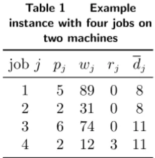
Table 1 Example instance with four jobs on
two machines jobj pj wj rj dj 1 5 89 0 8 2 2 31 0 8 3 6 74 0 11 4 2 12 3 11
under this ordering. The ZDD will follow the same ordering. Define sumj=
Pn
i=jpj and
mj= min{pi|j ≤i≤n}. A configuration (j, t) of a nonterminal node is a pair consisting
of a job index j and the total processing time t of all the processed jobs i with i < j, in other words t is the starting time of jobj. The 1- and 0-node are represented respectively by (n+ 1,1) and (n+ 1,0). FunctionROOTS() returns configuration (1,0), and procedure
CHILDS((j, t), b) is described in Algorithm 2. Each node (j, t) in the DD apart from the
terminal nodes has two child nodes. The high edge representing inclusion of jobj leads to (j0, t+pj), where j0 is the job with the smallest index greater than j for whichrj0 ≤t+pj
and t+pj+pj0≤dj0. The low edge (exclusion of job j) leads to configuration (j0, t), where
j0 is a job with similar properties. If no such job j0 exists, the high edge points to the
1-node if t+pj ∈[Hmin;Hmax] and to the 0-node otherwise. For the low edge, the same
holds but based on the value of t instead of t+pj.
In Section 5.1 we mentioned that nodes in the DD associated with the same job can be merged if they have the same low and high child. We also implement this reduction process, but we note that different configurations (j, t) and (j, t0) might be merged in this way, pointing to different possible starting times t and t0 for the job j. These starting times are important for the determination of the cost of the schedules (and also constitute sufficient information). Therefore, with every node p of ZS we associate the set Tp as the
set of all possible starting times of job v(p). These sets can be easily calculated with a top-down/breadth-first method starting at the root node of ZS.
We illustrate the foregoing by means of a small example withn= 4 and m= 2, for which
Hmin= 7 andHmax= 11; further data are shown in Table 1. Figure 1 visualizes the different
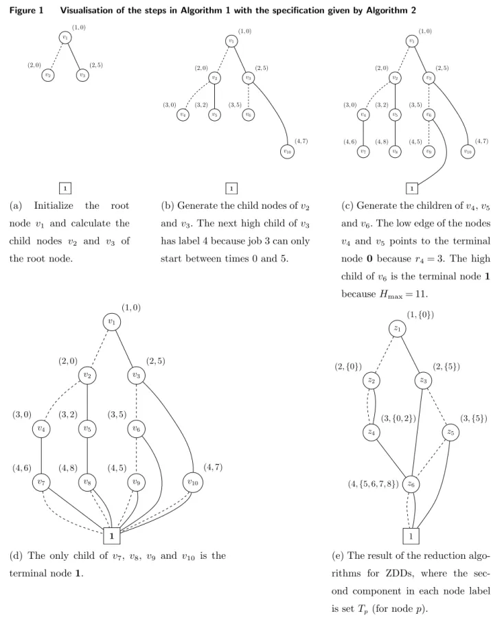
steps of Algorithm 1 for the recursive specification in Algorithm 2. The number of nodes in the ZDD in Figure 1(e) is clearly lower than the DD in Figure 1(d), before the reduction. Solving phase In each iteration of the CG procedure we will be searching for a variable with negative reduced cost. Hence we must associate to each 1-path of ZS, i.e. to each
Figure 1 Visualisation of the steps in Algorithm 1 with the specification given by Algorithm 2 v1 v2 v3 v10 1 (1,0) (2,0) (2,5)
(a) Initialize the root node v1 and calculate the
child nodes v2 and v3 of
the root node.
v1 v2 v3 v4 v5 v6 v10 1 (1,0) (2,0) (2,5) (3,0) (3,2) (3,5) (4,7)
(b) Generate the child nodes ofv2
andv3. The next high child of v3
has label 4 because job 3 can only start between times 0 and 5.
v1 v2 v3 v4 v5 v6 v7 v8 v9 v10 1 (1,0) (2,0) (2,5) (3,0) (3,2) (3,5) (4,6) (4,8) (4,5) (4,7)
(c) Generate the children ofv4,v5
andv6. The low edge of the nodes v4 and v5 points to the terminal
node 0 because r4= 3. The high
child of v6 is the terminal node1
because Hmax= 11. v1 v2 v3 v4 v5 v6 v7 v8 v9 v10 1 (1,0) (2,0) (2,5) (3,0) (3,2) (3,5) (4,6) (4,8) (4,5) (4,7)
(d) The only child of v7, v8, v9 and v10 is the
terminal node1. z1 z6 1 z4 z5 z2 z3 (1,{0}) (2,{0}) (2,{5}) (3,{0,2}) (3,{5}) (4,{5,6,7,8})
(e) The result of the reduction algo-rithms for ZDDs, where the sec-ond component in each node label is set Tp (for nodep).
Algorithm 2: Calculation of all reachable configurations of S Function CHILDS((j, t), b) if b= 1 then t0←t+pj; else t0←t; j0←M IN J OB(j, t0); if j0≤n then
if t0+sumj0< Hmin then
return (n+ 1,0);
if t0∈[Hmin, Hmax] and t0+mj0 > Hmax then
return (n+ 1,1);
else
if t0∈[Hmin, Hmax] then
return (n+ 1,1);
return (n+ 1,0)
return (j0, t0);
Function M IN J OB(j, t)
if min{i > j|t∈[ri, di−pi]} exists then
return min{i > j|t∈[ri, di−pi]};
return n+ 1;
path from the root node to the 1-node, a value that is equal to the reduced cost of the associated schedule. We implicitly find a path with lowest reduced cost by means of a DP algorithm, which is different from the one presented in Morrison et al. (2016b) because the cost associated to each column (schedule) is nonlinear in function of the job selection. The pricing problem in Morrison et al. (2016b) was a binary combinatorial optimization problem with a linear function, because the cost associated to every variable of the RMP was equal to 1, and then the pricing problem was equivalent to finding a shortest path. In
our case, the nonlinearity is removed by explicitly considering each possible starting time for each job in the definition of a configuration.
Let (π, σ) be an optimal dual vector of the RMP at some iteration of the CG, and letZS be a ZDD that represents the family of sets S. Let |ZS| be the size of ZS (the number of nodes) andz1, . . . , z|ZS|its nodes, wherez1 is the root node, andz|ZS|−1 andz|ZS|correspond
to the 1- and 0-node, respectively. We also assume that each parent node zi has a lower
index i than its child nodes. In the DP algorithm we fill (only the relevant entries of) two tables O and B of size |ZS| ×Hmax. ValueO[k][t] represents the minimal reduced cost
of a partial schedule that starts with job v(k) (the job associated to node k) at time t, minimized over all partial schedules that can execute jobs in{v(k), v(k) + 1, . . . , n}, where a partial schedule contiguously executes a set of jobs from a time instant greater than or equal to zero onwards. The reduced cost of a partial schedule is its contribution to the reduced cost of a schedules∈ S that contains the partial schedule. This value is associated with a path from configuration (v(k), t) to the 1-node before the reduction of the DD. Thus, we seek to determine O[z1][0].
Stepwise, we fill the tables by traversing ZS from the terminal nodes to the root node; Algorithm 3 illustrates this process. For each nodek and starting timet, we store the best choice (selection or not of job v(k), corresponding to values 1 and 0) in B[k][t]. We do not examine all values for t ranging from rv(k) to dv(k)−pv(k), but we only consider values
in set Tk. We compare O[hi(zi)][t+pv(zi)]−πv(zi)+wv(zi)(t+pv(zi)) and O[lo(zi)][t] for all
t∈Tzi, and we set O[zi][t] to be the minimum of the two.
6.
Farkas pricing
The Farkas lemma is an important result of LP that implies, with the column set S0⊂ S in the RMP, that exactly one of the following two statements is true:
1. ∃λ∈R|S0|
such that Equations (6b) and (6c) hold, or 2. ∃π∈Rn
+ and σ∈R+ such that ∀s∈ S0:
P
j∈sπj−σ≤0 and
P
j∈Jπj−mσ >0.
Therefore, if our RMP is infeasible then there exists a vector (π, σ), which can be inter-preted as a ray in the dual, proving the infeasibility of the RMP. With CG we can now try to render the formulation feasible by adding a variable λs such that
P
j∈sπj−σ >0,
i.e., we destroy the proof of infeasibility by the inclusion of this λs. Such a variable can
Algorithm 3: DP algorithm based on ZS for the pricing problem
Data: ZDD ZS, optimal solution (π, σ) of the dual
Result: Schedule s of S with most negative reduced cost
O[z|ZS|−1][t]←σ for all t∈Tz|ZS |−1;
O[z|ZS|][t]←+∞ for all t∈Tz|ZS |;
for i=|ZS| −2 to 1 do
for t∈Tzi do
if O[hi(zi)][t+pv(zi)]−πv(zi)+wv(zi)(t+pv(zi))≥O[lo(zi)][t] then
O[zi][t]←O[lo(zi)][t]; B[zi][t]←0; else O[zi][t]←O[hi(zi)][t+pv(zi)]−πv(zi)+wv(zi)(t+pv(zi)); B[zi][t]←1; z←z1, t←0 and s← ∅; while z6=z|ZS|−1 do if B[z][t] = 0 then s←s∪ {v(z)}, t←t+pv(z), z←hi(z); else z←lo(z);
pricing problem (9) but without the cost function cs. If the optimal objective value of this
pricing problem is positive, then we iteratively add the new variable to the restricted LP and solve it again, until we have shown that the LP relaxation is either feasible or infeasi-ble. Otherwise, if the optimal objective value of this new pricing problem is negative then we conclude that we cannot remove the infeasibility. This so-called Farkas pricing problem can again be solved using ZDDs. Since the schedule cost is not part of the objective, the problem equates to finding a longest path from the root node to the 1-node ofZS.
Our foregoing approach for resolving infeasibilities is different from the one in van den Akker et al. (1999). The latter authors add infeasible variables with a “big-M”-type penalty cost to the restricted LP relaxation, and thus at least one feasible solution always exists.
Selecting the value of these big-M penalties is difficult, however. LowerM leads to tighter upper bounds on the respective dual variables and may reduce the so-called “heading-in” effect of initially produced irrelevant columns (due to the lack of compatibility of the initial column pool with the newly added columns). Additionally, van den Akker et al. (1999) also use a number of heuristics in order to test whether or not there exists a feasible solution.
7.
Stabilization techniques
It is well known that the convergence of a CG algorithm for scheduling problems can be slow due to primal degeneracy; this situation can be improved by using stabilization techniques. One of these techniques is dual-price smoothing, which was introduced in Wentges (1997). This technique corrects the optimal solution of the dual problem of the restricted LP relaxation based on past information before it is plugged into the pricing algorithm. We first introduce a number of concepts before the stabilization technique itself can be explained. We first describe a dual bound for the LP relaxation of (6), in which we relax the covering constraints (6b). This leads to the following Lagrangian subproblem for any Lagrangian penalty vector π∈Rn +: minimize X s∈S (cs− X j∈s πj)λs+ X j∈J πj (10a) subject to X s∈S λs≤m (10b) λs≥0 for each s∈ S (10c)
Using equations (10b) and (10c) we obtain that the Lagrangian dual function L:Rn→R
of the Lagrangian relaxation is given by:
L(π) = min ( 0,min s∈S{cs− X j∈s πj}m ) +X j∈J πj (11)
for every Lagrangian penalty vectorπ∈Rn
+. From (11) we deduce that each time the pricing
problem (9) is solved for a dual vector π, we immediately also obtain the dual boundL(π) associated to that dual vector. Maximizing the Lagrangian dual function overπ∈Rn
+ gives
the best possible dual bound that can be derived from the Lagrangian relaxation; this is called the Lagrangian dual bound. We define the Lagrangian dual problem as:
max
π∈Rn+
which is a max-min problem. Formulating this max-min problem as a linear program will give us a relation between the Lagrangian dual bound and the lower bound obtained from the LP relaxation of (6): max π∈Rn + L(π) = max π∈Rn + ( X j∈J πj+ min ( 0, mmin s∈S{cs− X j∈s πj} )) = max ( X j∈J πj−mσ π∈Rn +,−σ≤0 and −σ≤cs− X j∈s πj,∀s∈ S ) = min ( X s∈S csλs X s∈S:j∈s λs≥1,∀j∈J, X s∈S λs≤m and λs≥0,∀s∈ S ) .
In this way we see that the Lagrangian dual bound is equal to the bound obtained by the LP relaxation of (6).
Wentges (1997) proposes not to simply use the last-obtained vector ¯π∈Rn
+of dual prices
associated to the covering constraints (6b) of the restricted master in every iteration of the CG, but rather to smoothen these dual prices into the direction of the stability center, which is the dual solution ˆπ that has generated the best dual bound ˆL=L(ˆπ) so far (over the different iterations of the CG). Wentges (1997) uses the following dual-price smoothing rule:
e
π:=απˆ+ (1−α)¯π= ˆπ+ (1−α)(¯π−πˆ). (13) This vector is plugged into the pricing problem, with α∈[0,1). Define by es an optimal solution of problem (9) with respect toπeand let ¯σbe the last-obtained dual price associated to constraint (6c) in the restricted master. If es has negative reduced cost with respect to ¯π (i.e., ces−
P
j∈es
¯
πj+ ¯σ <0), then the corresponding column λse can be added to the
RMP. Moreover, the stability center ˆπ is updated each time the Lagrangian bound L(eπ) = min{0, m(c
e
s−Pj∈ese
πj)}+Pj∈Jeπj is improved: ifL(eπ)>Lˆ then we update ˆπ:=eπ. This is
repeated untilP
j∈Jπ¯j−mσ¯−L < ˆ with >0 and sufficiently small. We call this stabilized
column generation.
Remark that the pricing problem with smoothed dual vector πe might not yield a new variable with negative reduced cost, i.e., c
e
s−Pj∈es
¯
π+ ¯σ≥0 even if such a variable can be found with the optimal dual vector (¯π,σ¯). We call such a situation misspricing. With the following lemma one can show that the number of missprices is polynomially bounded:
Lemma 1 (Pessoa et al., 2010). If misspricing occurs for eπ, then P
j∈J¯π−mσ¯−L(eπ)≤
α(P
j∈Jπ¯−mσ¯−Lˆ).
Hence we have that each missprice guarantees that the gap between the primal bound
P
j∈J¯πj−mσ¯ and the dual bound ˆL is reduced by at least a factor
1
α. Using Lemma 1
one can show now that stabilized CG is correct, meaning that the number of iterations in stabilized GCG is finite and that the procedure finishes with an optimal solution of the LP relaxation of (6) ifis sufficiently small. This establishes that stabilized CG using Wentges (1997) smoothing is asymptotically convergent. For a complete proof we refer to Pessoa et al. (2015), where a link is made between dual-price smoothing and in-out separation (see also Ben-Ameur and Neto, 2007), and where it is shown that other dual-price smoothing schemes in the literature also lead to asymptotically convergent stabilized CG algorithms.
8.
Branching rules
At each node of the B&P tree we solve the LP relaxation of formulation (6) and obtain an optimal solutionλ∗. One of the following two cases will occur at every node: either the LP relaxation has an integral solution and the new solution can be stored, or the LP solution is fractional. In the second case, we apply a branching strategy to close the integrality gap and find an integer solution.
8.1. General
In van den Akker et al. (1999) it is shown that some fractional solutions can be transformed into an integral solution without much effort, using the following result:
Theorem 1. If for every job j∈J it holds that Cj(s) :=Cj is the same for every s∈ S
withλ∗s>0, then the schedule obtained by processingj in the execution interval[Cj−pj, Cj]
is feasible and has minimum cost.
The branching strategy of van den Akker et al. (1999) is also based on Theorem 1, and is applied if the LP solutionλ∗does not satisfy the conditions of the theorem. In that case, one can deduce from Theorem 1 that there exists at least one job j for which P
s∈SCj(s)λ∗s>
min{Cj(s)|λ∗s>0}; this job is called the fractional job. Using the previous property, the
authors design a binary B&B tree for which in every node the fractional job j is first identified and, if any, then two child nodes are created. The first child has the condition that the deadline dj = min{Cj(s)|λ∗s >0}, in the second child the release date of this
job becomes rj = min{Cj(s)|λ∗s>0} +1−pj. A convenient consequence of this partition
strategy is that the pricing algorithm proposed in van den Akker et al. (1999) can stay the same also in the child nodes. It may occur, however, that the newly constructed instance does not have feasible solutions, i.e., that there exists no solution for whichrj+pj≤Cj≤dj
for every job j∈J.
For set covering formulations such as (6), however, a more generic branching scheme can also be applied, which is based on the following observation: if the solution λ∗ of (6) is fractional, then there exists a job pair (j, j0) for which 0<P
s∈S:j,j0∈sλ∗s<1 (see Ryan
and Foster, 1981). One can now separate the fractional solution λ∗ using the disjunction
P
s∈S:j,j0∈sλ∗s≤0 or P
s∈S:j,j0∈sλ∗s ≥1. We call the first branch the DIFF child, in which
the jobsj and j0 cannot be scheduled on the same machine. The second branch is referred to as the SAME child, where the jobs j andj0 have to be scheduled on the same machine. Obviously, these constraints have implications for the pricing problem in the child nodes. 8.2. Constructing ZDDs for the child nodes
We showed in Section 5.2 how the pricing problem in the root node of the search tree can be solved with ZDDs that hold all the feasible schedules. Below we explain how to manipulate a ZDD after imposing branching constraints. First define for each s∈ S an
n-dimensional binary vector as with asj= 1 if j∈s, otherwiseasj= 0.
A ZDD for a child node in the B&B tree can be conceived as an intersection of two ZDDs, and so we can construct this ZDD by using the generic binary intersection operation ∩on ZDDs (see Minato, 1993). Suppose for example that we have ZS in the root node of the search tree, and we wish to constrain this family of sets by considering only schedules s
with asj =asj0. We first define the family FSAM E
j,j0 ={s⊂J|asj=asj0}, represented by the
ZDDZFSAM E
j,j0 . The ZDDZS∩ZF SAM E
j,j0 is then the ZDD of the SAME child of the root node. A similar construction can be set up for the ZDD of the DIFF child, where the family
FDIF F
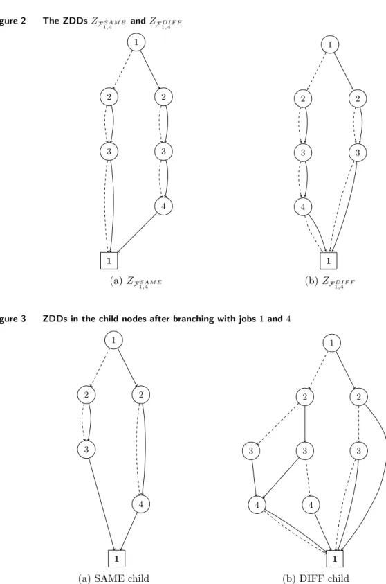
j,j0 ={s⊂J |asj+asj0≤1} can be used. In Figure 2 we depict the ZDDs ZFSAM E
1,4 and
ZFDIF F
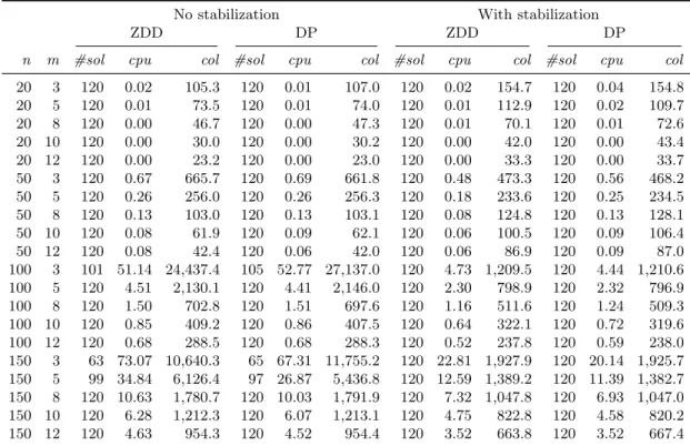
1,4 when |J|= 4. Figure 3 visualizes the ZDDs ZS∩ZF1SAM E,4 and ZS∩ZF1DIF F,4 for the instance of Table 1 (with ZS in Figure 1(e)).
In our implementation we deviate slightly from the foregoing description, in that we first compute the intersection of the recursive specifications and then construct the ZDD with Algorithm 1 given this specification; with this approach we follow Iwashita and Minato (2013). We first note that in a given node of the B&B tree we only know the ZDD Z and
Figure 2 The ZDDsZFSAM E 1,4 andZF1DIF F,4 1 4 1 3 3 2 2 (a)ZFSAM E 1,4 1 4 1 3 3 2 2 (b)ZFDIF F 1,4
Figure 3 ZDDs in the child nodes after branching with jobs 1and 4
1
4
1 3
2 2
(a) SAME child
1 4 4 1 3 3 2 2 3 (b) DIFF child
not its recursive specification, but Iwashita and Minato (2013) describe how to re-construct a recursive specification S for Z. The configuration in this case is a pair (i, p), where p
is a node of ZDD Z and i is the label of p. Clearly, the ROOTS function of S returns
function CHILDS of recursive specificationS with arguments (i, p) andb∈ {0,1} returns
(i0, p0), wherep0 is theb-child ofpandi0 is the label ofp0. These two functions are such that when one applies Algorithm 1 with recursive specification S, then this algorithm returns a ZDD that is equivalent to the original ZDD Z.
We now need to construct ZDDs for the child nodes of the B&B tree. For this we present a rather general recursive specification. Let (J, ESAM E) be an undirected graph that joins
two nodesj andj0 if they have to be scheduled on the same machine, and (J, EDIF F) is an
undirected graph that joins two nodes j and j0 if they have to be scheduled on different machines. Let
FSAM E={s⊂J|asj=asj0,∀{j, j0} ∈ESAM E}
and
FDIF F ={s⊂J|asj+asj0 ≤1,∀{j, j0} ∈EDIF F}.
We derive a recursive specification SFSAM E∩FDIF F for FSAM E ∩ FDIF F. For every j∈J, define Aj as the set {j0∈J | {j, j0} ∈ESAM E} and Bj as the set {j0∈J| {j, j0} ∈EDIF F}.
The configurations for recursive specificationSFSAM E∩FDIF F are pairs (j,(SADD, SREM OV E)) wherej∈J,SADD⊂J is a job set that contains all the jobs have that to be added based on
the choices made higher in the ZDD, and SREM OV E⊂J contains all the jobs that cannot
be added based on the previous choices. The configurations of the 1-node and the 0-node are defined as before. The function ROOTSFSAM E∩FDIF F returns a pair for which the first
component is 1 and the second component is (∅,∅). The function CHILDSFSAM E∩FDIF F is
summarized as Algorithm 4.
The ZDD of the child nodes in the B&B algorithm can now be set up as follows. Suppose that we apply the generic branching scheme on the jobs j and j0. Let Z be the ZDD at the parent node andS its recursive configuration. The ZDD of the SAME child is the out-put of Algorithm 1 with recursive specification S∩SSAM E, where SSAM E=SFSAM E∩FDIF F with FSAM E ={s⊂J |asj =asj0} and FDIF F = 2J. The ZDD of the DIFF child can be
obtained similarly with recursive specification S∩SSAM E, where SSAM E=SFSAM E∩FDIF F with FDIF F ={s⊂J|asj+asj0≤1} and FSAM E= 2J.
8.3. Branching choice
It is very important to make a good choice for the branching jobsj andj0. This choice has a great influence on the computation time of the algorithm, partly because it decides how
Algorithm 4: Calculation of all reachable configurations of FSAM E∩ FDIF F
Function CHILDS((j,(SADD, SREM OV E)), b)
if Aj∩Bj6=∅ then return (n+ 1,0) if b= 1 then if j∈SREM OV E then return (n+ 1,0); SADD0 ←SADD∪Aj; SREM OV E0 ←SREM OV E∪Bj; else if j∈SADD then return (n+ 1,0); SREM OV E0 ←SREM OV E∪Aj; j0←min({i > j|i∈SREM OV E0 } ∪ {n+ 1}); if j0=n+ 1 and b then if j /∈SREM OV E then return (n+ 1,1); return (n+ 1,0) else if j /∈SADD then return (n+ 1,1); return (n+ 1,0)
return (j0,(SADD0 , SREM OV E0 ))
the B&B algorithm traverses the search tree, but also because it has an impact on the size of the ZDD in the pricing problem.
In our first experiments we used a selection criterion that was introduced by Held et al. (2012) for the vertex coloring problem, but which can be applied to every set covering formulation. For each job pair{j, j0} define
p(j, j0) = P s∈S:j,j0∈sλs 1 2( P s∈S:j∈sλs+ P s∈S:j0∈sλs) . (14)
For all pairs j, j0 we have that p(j, j0)∈[0,1] and the value is well defined. When p(j, j0) is close to 0 then jobs j and j0 tend to be assigned to different machines in the fractional solution, whereas if p(j, j0) is close to 1, then j and j0 are mostly assigned to the same machines. Therefore, it is preferable to choose a pair j, j0 for which the value p(j, j0) is (the) close(st) to 0.5, because otherwise the lower bound of child nodes will probably not radically change.
We noticed that the size of the ZDDs of the child nodes typically grows quite fast when this selection criterion is applied. This is not very surprising because the imposed constraints severely change the structure of the pricing problem in the child nodes. This growth in size can be controlled, however, by choosing a branching pair j, j0 such that the difference between j and j0 is small, and this is an extra aspect that we would like to take along in the branching choice. Assume thatj < j0. Based on some preliminary experiments, we have come up with the following heuristic priority value:
s(j, j0) =|p(j, j0)−q(j, j0) + (j0−j)r(j, j0)|, (15) and we choose a job pair {j, j0} such that s(j, j0) is minimal. In this expression,
q(j, j0) = X s∈S:j,j0∈s 0.5− |λs− bλsc −0.5| |{s∈ S|j, j0∈s}| (16) and r(j, j0) = |p(j, j 0)−q(j, j0)|+ n×r(j, j0) . (17)
The underlying reasoning is that we wish to give priority to job pairs for which (1) the difference betweenj andj0 is small, which is achieved by adding the term (j0−j)r(j, j0) to
p(j, j0); and (2) the distance betweenp(j, j0) andq(j, j0) is small, which means that the jobs
j and j0 do not frequently appear on the same machine in the pool of generated columns that have a non-zero λ–value.
9.
Computational experiments
9.1. Experimental setup
We have implemented two B&P algorithms, referred to as VHV and RF below, which mainly differ in their branching strategy. VHV uses the branching strategy of van den Akker et al. (1999), but contrary to the original reference our implementation applies Farkas pricing to solve infeasibilities (see Section 6). The pricing problem is solved either
with the DP algorithm presented in van den Akker et al. (1999) or with a ZDD, leading to the variants VHV-DP and VHV-ZDD, respectively. In VHV-ZDD we build a new ZDD that represents the set of feasible schedules with the new time windows at every node of the B&B tree. RF applies the generic branching scheme of Ryan and Foster (1981); the pricing problem is solved with ZDDs as explained in Sections 5.2 and 8.2.
The algorithms have been implemented in the C++ programming language and compiled with gcc version 5.4.0 with full optimization pack -O5. We have used and adjusted the implementation of Iwashita and Minato (2013) that can be found on Github1 to construct the ZDDs. The computational experiments have been performed on one core of a system with Intel Core i7–3770 processor at 3.4 GHz and 8 GB of RAM under a Linux OS. All LPs are solved with Gurobi 6.5.2 using default settings and only one core.
We test the algorithms on six classes of randomly generated instances, as follows: class 1: pj∼U[1,10] and wj∼U[10,100]; class 2: pj∼U[1,100] and wj∼U[1,100]; class 3: pj∼U[10,20] and wj∼U[10,20]; class 4: pj∼U[90,100] andwj∼U[90,100]; class 5: pj∼U[90,100] and wj∼U[pj−5, pj+ 5]; class 6: pj∼U[10,100] and wj∼U[pj−5, pj+ 5].
With these settings we follow van den Akker et al. (1999, 2002). We generate instances withn= 20,50,100 and 150 jobs andm= 3,5,8,10 and 12 machines. For each combination of n, m and instance class we construct 20 instances.
9.2. Comparison of pricing algorithms and effect of stabilization
We first compare the different pricing algorithms only in the root node of the B&B tree. Each run is interrupted after 200 seconds. Note that the pricing algorithms in RF and VHV-ZDD are identical in the root node. Table 2 contains a summary of our findings. In this table,#sol is the number of instances out of 120 for which an optimal solution for the LP relaxation is found within 200 seconds, col is the average number of generated columns over these solved instances and cpu is the average CPU time (in seconds) over the solved instances.
From Table 2 we conclude that both for the case with and the case without stabilization, the runtimes for the DP solver and for the ZDD solver are more less comparable in the 1
Table 2 Computation of lower bound in the root node
No stabilization With stabilization
ZDD DP ZDD DP
n m #sol cpu col #sol cpu col #sol cpu col #sol cpu col
20 3 120 0.02 105.3 120 0.01 107.0 120 0.02 154.7 120 0.04 154.8 20 5 120 0.01 73.5 120 0.01 74.0 120 0.01 112.9 120 0.02 109.7 20 8 120 0.00 46.7 120 0.00 47.3 120 0.01 70.1 120 0.01 72.6 20 10 120 0.00 30.0 120 0.00 30.2 120 0.00 42.0 120 0.00 43.4 20 12 120 0.00 23.2 120 0.00 23.0 120 0.00 33.3 120 0.00 33.7 50 3 120 0.67 665.7 120 0.69 661.8 120 0.48 473.3 120 0.56 468.2 50 5 120 0.26 256.0 120 0.26 256.3 120 0.18 233.6 120 0.25 234.5 50 8 120 0.13 103.0 120 0.13 103.1 120 0.08 124.8 120 0.13 128.1 50 10 120 0.08 61.9 120 0.09 62.1 120 0.06 100.5 120 0.09 106.4 50 12 120 0.08 42.4 120 0.06 42.0 120 0.06 86.9 120 0.09 87.0 100 3 101 51.14 24,437.4 105 52.77 27,137.0 120 4.73 1,209.5 120 4.44 1,210.6 100 5 120 4.51 2,130.1 120 4.41 2,146.0 120 2.30 798.9 120 2.32 796.9 100 8 120 1.50 702.8 120 1.51 697.6 120 1.16 511.6 120 1.24 509.3 100 10 120 0.85 409.2 120 0.86 407.5 120 0.64 322.1 120 0.72 319.6 100 12 120 0.68 288.5 120 0.68 288.3 120 0.52 237.8 120 0.59 238.0 150 3 63 73.07 10,640.3 65 67.31 11,755.2 120 22.81 1,927.9 120 20.14 1,925.7 150 5 99 34.84 6,126.4 97 26.87 5,436.8 120 12.59 1,389.2 120 11.39 1,382.7 150 8 120 10.63 1,780.7 120 10.03 1,791.9 120 7.32 1,047.8 120 6.93 1,047.0 150 10 120 6.28 1,212.3 120 6.07 1,213.1 120 4.75 822.8 120 4.58 820.2 150 12 120 4.63 954.3 120 4.52 954.4 120 3.52 663.8 120 3.52 667.4
root node. In the next section we will see that the ZDD solver will nevertheless usually be preferable, by the fact that the RF branching strategy requires less nodes for finding an optimal solution.
The stabilization itself has a beneficial effect especially when the number of jobs per machine is high, so for high ratio n/m. The number of generated columns is also much lower for instances with high n/m. This will also have an important effect for identifying integral solutions at lower levels of the B&B tree.
9.3. Computational results
We will compare the three algorithms VHV-ZDD, VHV-DP and RF. Each run of the algorithm (for one instance) is interrupted after 3600 seconds. We first report the results aggregated over the six instances classes, and subsequently we discuss the detailed perfor-mance per class.
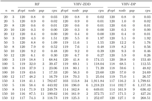
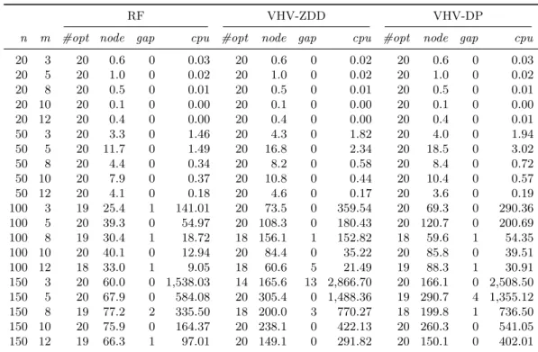
Overall computational results Table 3 shows the overall performance of the three algo-rithms. The columns labeled#opt contain the number of solved instances out of 120 within one hour, node is the average number of explored nodes of the B&B tree over the solved instances, cpu is the average CPU time over the solved instances (in seconds), and gap is the maximum absolute gap over the unsolved instances.
Table 3 Comparison of the B&P algorithms aggregated over the six instance classes
RF VHV-ZDD VHV-DP
n m #opt node gap cpu #opt node gap cpu #opt node gap cpu
20 3 120 0.8 0 0.03 120 0.8 0 0.02 120 0.8 0 0.03 20 5 120 0.9 0 0.02 120 0.9 0 0.01 120 1.0 0 0.02 20 8 120 0.6 0 0.01 120 0.6 0 0.01 120 0.6 0 0.01 20 10 120 0.3 0 0.00 120 0.3 0 0.00 120 0.3 0 0.00 20 12 120 0.4 0 0.00 120 0.4 0 0.00 120 0.4 0 0.01 50 3 120 4.3 0 1.51 120 5.5 0 1.97 120 5.1 0 1.92 50 5 120 8.8 0 1.09 119 11.6 1 1.55 120 12.2 0 1.76 50 8 120 7.9 0 0.52 119 7.6 1 0.48 119 8.2 1 0.56 50 10 120 9.2 0 0.48 120 9.2 0 0.39 120 9.3 0 0.46 50 12 120 6.1 0 0.30 120 6.7 0 0.27 120 5.9 0 0.26 100 3 119 18.8 1 68.84 120 41.8 0 174.15 120 39.8 0 153.40 100 5 119 32.0 3 39.47 119 69.1 1 118.04 118 68.5 1 112.55 100 8 118 37.9 1 23.06 118 80.1 1 71.39 118 59.6 1 48.82 100 10 119 43.6 1 17.33 120 56.3 0 23.60 120 57.0 0 24.69 100 12 117 48.2 1 16.79 118 70.3 5 25.04 119 75.0 1 26.57 150 3 118 41.1 1 782.67 103 113.8 34 1,911.84 117 116.2 3 1,799.61 150 5 116 58.4 6 443.92 116 196.0 6 1,218.23 114 192.7 6 1,157.16 150 8 114 71.9 13 249.78 114 162.8 6 649.01 114 161.9 9 636.42 150 10 116 87.5 11 199.62 116 161.9 2 372.75 117 171.5 2 427.24 150 12 117 74.3 3 116.73 119 125.3 1 252.07 120 127.1 0 268.51
We first notice that the branching scheme RF needs to explore less nodes on average to find an optimal solution. This has a great impact on the total runtime, and leads to better results especially when the number of jobs per machine is high. Consequently, not only stabilization contributes to the efficiency of the algorithm, but also the branching scheme is of vital importance. We also see that algorithm VHV-DP solves slightly more instances to optimality. The reason why algorithm RF sometimes fails to find optimal solutions is probably a bad exploration of the B&B tree: we use a hybrid depth-first approach and one of the problems associated with depth-first exploration is trashing, which occurs when different regions of the search fail for the same or similar reason, see for instance Morrison et al. (2016a). For example a single constraint can lead to infeasibility, but this infeasibility is only detected after exploration of subproblems deeper in the B&B tree.
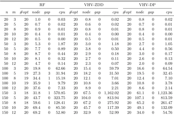
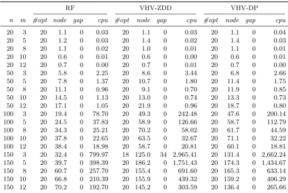
Computational results for class 1 Table 4 pertains to 20 instances instead of 120. The table shows that the algorithms perform well on the first class of instances. Algorithms VHV-ZDD and VHV-DP solve all the instances to optimality and the average CPU time tends to be smaller than for RF, unless the ratio mn is at least 18. For instances with the latter property, it becomes more difficult for algorithms VHV-ZDD and VHD-DP to find an optimal solution, the search requires more nodes for these instances and algorithm RF
Table 4 Comparison of the B&P algorithms: Class 1
RF VHV-ZDD VHV-DP
n m #opt node gap cpu #opt node gap cpu #opt node gap cpu
20 3 20 1.0 0 0.03 20 0.8 0 0.02 20 0.8 0 0.02 20 5 20 0.7 0 0.02 20 0.6 0 0.02 20 0.7 0 0.01 20 8 20 0.9 0 0.01 20 0.8 0 0.01 20 0.8 0 0.01 20 10 20 0.4 0 0.01 20 0.4 0 0.00 20 0.4 0 0.00 20 12 20 0.5 0 0.00 20 0.5 0 0.01 20 0.5 0 0.01 50 3 20 5.3 0 1.87 20 3.0 0 1.18 20 2.7 0 1.05 50 5 20 7.7 0 0.89 20 3.8 0 0.50 20 4.4 0 0.56 50 8 20 8.7 0 0.44 20 2.9 0 0.18 20 3.0 0 0.17 50 10 20 8.1 0 0.32 20 2.7 0 0.11 20 2.6 0 0.13 50 12 20 4.7 0 0.14 20 2.3 0 0.07 20 2.0 0 0.09 100 3 20 19.8 0 62.66 20 15.4 0 59.79 20 16.6 0 64.54 100 5 19 27.3 3 31.94 20 18.2 0 31.50 20 19.5 0 32.45 100 8 19 34.4 1 15.18 20 12.1 0 7.01 20 12.4 0 7.10 100 10 19 35.9 1 9.79 20 10.8 0 3.66 20 10.8 0 3.78 100 12 20 37.6 0 7.33 20 8.9 0 2.21 20 8.6 0 2.14 150 3 18 31.8 1 570.85 20 67.5 0 1,162.02 20 61.1 0 1,123.36 150 5 20 43.7 0 323.75 20 104.0 0 813.94 20 107.1 0 813.59 150 8 18 59.6 1 128.41 20 67.2 0 275.92 20 65.2 0 261.47 150 10 20 69.4 0 85.50 20 45.7 0 117.39 20 49.1 0 132.09 150 12 20 69.2 0 52.80 20 32.9 0 52.99 20 34.0 0 54.76
finds optimal solutions more quickly. When the ratio mn becomes bigger we have to set tighter time windows for more jobs.
Computational results for class 2 The first major difference with class 1 is that the lower bound at the root node for class 2 is not tight when the number of machines and jobs increases, because we obtain more fractional solutions. The number of explored nodes also grows, and thus the average runtime also goes up. Clearly, the values of wj
pj for every
j∈J are often different from each other and the final position of every job on its assigned machine is very clear. Consequently, the assignment of the jobs becomes very important for these instances. We have chosen the weights and the processing times from the uniform distribution U[1,100]. Because of this the number of fractional solutions grows and hence the set covering formulation is less tight. Moreover, the average size of the ZDDs for this class of instances is significantly larger than for class 1 (see Section 9.4). Overall, all three the algorithms solve the problem very well and the average CPU time is small. Algorithm RF performs best especially on instances with 150 jobs.
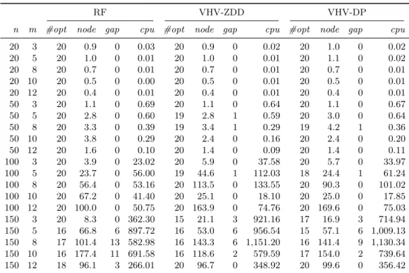
Computational results for class3 For instances in this class the processing timepj and
weight wj for everyj∈J are close to each other, and so the ratio between the weight and
Table 5 Comparison of the B&P algorithms: Class 2
RF VHV-ZDD VHV-DP
n m #opt node gap cpu #opt node gap cpu #opt node gap cpu
20 3 20 0.9 0 0.03 20 0.9 0 0.02 20 1.0 0 0.02 20 5 20 1.0 0 0.01 20 1.0 0 0.01 20 1.1 0 0.02 20 8 20 0.7 0 0.01 20 0.7 0 0.01 20 0.7 0 0.01 20 10 20 0.5 0 0.00 20 0.5 0 0.01 20 0.5 0 0.01 20 12 20 0.4 0 0.01 20 0.4 0 0.01 20 0.4 0 0.01 50 3 20 1.1 0 0.69 20 1.1 0 0.64 20 1.1 0 0.67 50 5 20 2.8 0 0.60 19 2.8 1 0.59 20 3.0 0 0.64 50 8 20 3.3 0 0.39 19 3.4 1 0.29 19 4.2 1 0.36 50 10 20 3.8 0 0.29 20 2.4 0 0.16 20 2.4 0 0.20 50 12 20 1.6 0 0.10 20 1.4 0 0.09 20 1.4 0 0.11 100 3 20 3.9 0 23.02 20 5.9 0 37.58 20 5.7 0 33.97 100 5 20 23.7 0 56.00 19 44.6 1 112.03 18 24.4 1 61.24 100 8 20 56.4 0 53.16 20 113.5 0 133.55 20 90.3 0 101.02 100 10 20 67.2 0 41.40 20 25.1 0 18.10 20 25.0 0 17.85 100 12 20 100.0 0 50.75 20 163.9 0 74.76 20 169.6 0 75.03 150 3 20 8.3 0 362.30 15 21.1 3 921.16 17 16.9 3 714.94 150 5 16 66.8 6 897.72 16 53.0 6 956.54 15 57.1 6 1,009.13 150 8 17 101.4 13 582.98 16 143.3 6 1,151.20 16 141.4 9 1,130.34 150 10 16 177.4 11 691.58 16 118.6 2 579.59 17 154.0 2 739.64 150 12 18 96.1 3 266.01 20 96.7 0 348.92 20 99.6 0 356.42
will be many relevant feasible schedules. The algorithms VHV-DP and VHV-ZDD perform quite weakly on these instances; this was already observed in van den Akker et al. (1999). It is nevertheless surprising that the algorithms require a long time for finding a feasible solution, because the formulation is very tight. This can be explained by the fact that the set covering formulation often returns a fractional solution. The branching strategy of RF clearly needs less nodes to find an optimal solution and hence the average runtime over the solved instances is lower. We conjecture that in general, the positions of the jobs in the final solution are more predetermined by assigning two jobs to the same machine, rather than by tightening the time window of one job.
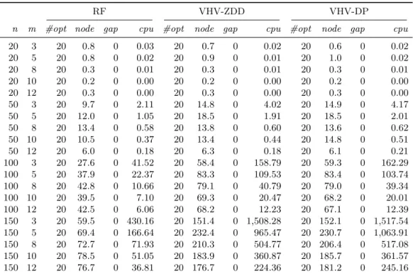
Computational results for class 4 These instances have the same properties as the previous class, only the processing times and the weights are larger. Table 7 shows that this class requires higher average runtime than class 3 for algorithms RF and VHV-ZDD. The same number of nodes is explored to find an integer solution, so the higher average computation time can only be explained by the size of the ZDDs, which determines the running time of the pricing problem; see our discussion in Section 9.4.
Computational results for class 5 These instances have the same properties as the previous class, but the different values wj
Table 6 Comparison of the B&P algorithms: Class 3
RF VHV-ZDD VHV-DP
n m #opt node gap cpu #opt node gap cpu #opt node gap cpu
20 3 20 0.8 0 0.03 20 0.7 0 0.02 20 0.6 0 0.02 20 5 20 0.8 0 0.02 20 0.9 0 0.01 20 1.0 0 0.02 20 8 20 0.3 0 0.01 20 0.3 0 0.01 20 0.3 0 0.01 20 10 20 0.2 0 0.00 20 0.2 0 0.00 20 0.2 0 0.00 20 12 20 0.3 0 0.00 20 0.3 0 0.00 20 0.3 0 0.00 50 3 20 9.7 0 2.11 20 14.8 0 4.02 20 14.9 0 4.17 50 5 20 12.0 0 1.05 20 18.5 0 1.91 20 18.5 0 2.01 50 8 20 13.4 0 0.58 20 13.8 0 0.60 20 13.6 0 0.62 50 10 20 10.5 0 0.37 20 13.4 0 0.44 20 14.8 0 0.51 50 12 20 6.0 0 0.18 20 6.3 0 0.18 20 6.1 0 0.21 100 3 20 27.6 0 41.52 20 58.4 0 158.79 20 59.3 0 162.29 100 5 20 37.9 0 22.37 20 83.3 0 109.53 20 83.4 0 103.74 100 8 20 42.8 0 10.66 20 79.1 0 40.79 20 79.0 0 39.34 100 10 20 39.5 0 7.10 20 69.3 0 20.47 20 68.2 0 20.01 100 12 20 42.5 0 6.06 20 68.2 0 12.23 20 67.1 0 12.39 150 3 20 59.5 0 430.16 20 151.4 0 1,508.28 20 152.1 0 1,517.54 150 5 20 69.4 0 166.64 20 232.4 0 965.47 20 230.7 0 1,063.91 150 8 20 72.7 0 71.93 20 210.3 0 504.77 20 206.4 0 517.08 150 10 20 78.5 0 51.05 20 183.9 0 360.87 20 185.7 0 361.57 150 12 20 76.7 0 36.81 20 176.7 0 224.36 20 181.2 0 245.16
Table 7 Comparison of the B&P algorithms: Class 4
RF VHV-ZDD VHV-DP
n m #opt node gap cpu #opt node gap cpu #opt node gap cpu
20 3 20 0.6 0 0.03 20 0.6 0 0.02 20 0.7 0 0.03 20 5 20 0.7 0 0.01 20 0.7 0 0.01 20 0.7 0 0.01 20 8 20 0.5 0 0.01 20 0.5 0 0.01 20 0.5 0 0.01 20 10 20 0.2 0 0.00 20 0.2 0 0.00 20 0.2 0 0.00 20 12 20 0.5 0 0.00 20 0.5 0 0.00 20 0.5 0 0.00 50 3 20 0.9 0 0.70 20 1.0 0 0.69 20 1.5 0 1.01 50 5 20 10.7 0 1.17 20 16.6 0 2.13 20 17.3 0 2.59 50 8 20 6.5 0 0.42 20 8.1 0 0.49 20 7.8 0 0.62 50 10 20 10.3 0 0.39 20 12.9 0 0.45 20 12.6 0 0.62 50 12 20 3.1 0 0.13 20 3.6 0 0.13 20 3.5 0 0.17 100 3 20 17.1 0 69.73 20 48.8 0 186.70 20 40.3 0 169.07 100 5 20 39.1 0 33.34 20 100.3 0 147.82 20 99.8 0 159.27 100 8 20 29.0 0 14.84 20 57.2 0 44.29 20 54.9 0 47.10 100 10 20 40.6 0 9.70 20 85.0 0 31.49 20 80.9 0 34.77 100 12 19 35.5 1 7.29 20 60.6 0 18.41 20 57.4 0 20.36 150 3 20 54.0 0 973.53 16 153.8 8 2,261.55 20 154.8 0 2,108.39 150 5 20 65.0 0 383.71 20 266.8 0 1,281.31 20 267.2 0 1,239.42 150 8 20 63.3 0 164.27 20 200.6 0 612.88 20 193.1 0 648.76 150 10 20 75.1 0 93.25 20 220.7 0 358.59 20 218.2 0 429.64 150 12 20 69.3 0 68.99 19 152.6 1 292.79 20 161.4 0 287.08
in the previous two instance classes. From Table 8 we see that the average CPU time of algorithm RF is lower than for algorithms VHV-ZDD and VHV-DP, but the average CPU time is higher than in the previous class. This can be explained by the fact that we need
Table 8 Comparison of the B&P algorithms: Class 5
RF VHV-ZDD VHV-DP
n m #opt node gap cpu #opt node gap cpu #opt node gap cpu
20 3 20 0.6 0 0.03 20 0.6 0 0.02 20 0.6 0 0.03 20 5 20 1.0 0 0.02 20 1.0 0 0.02 20 1.0 0 0.02 20 8 20 0.5 0 0.01 20 0.5 0 0.01 20 0.5 0 0.01 20 10 20 0.1 0 0.00 20 0.1 0 0.00 20 0.1 0 0.00 20 12 20 0.4 0 0.00 20 0.4 0 0.00 20 0.4 0 0.01 50 3 20 3.3 0 1.46 20 4.3 0 1.82 20 4.0 0 1.94 50 5 20 11.7 0 1.49 20 16.8 0 2.34 20 18.5 0 3.02 50 8 20 4.4 0 0.34 20 8.2 0 0.58 20 8.4 0 0.72 50 10 20 7.9 0 0.37 20 10.8 0 0.44 20 10.4 0 0.57 50 12 20 4.1 0 0.18 20 4.6 0 0.17 20 3.6 0 0.19 100 3 19 25.4 1 141.01 20 73.5 0 359.54 20 69.3 0 290.36 100 5 20 39.3 0 54.97 20 108.3 0 180.43 20 120.7 0 200.69 100 8 19 30.4 1 18.72 18 156.1 1 152.82 18 59.6 1 54.35 100 10 20 40.1 0 12.94 20 84.4 0 35.22 20 85.8 0 39.51 100 12 18 33.0 1 9.05 18 60.6 5 21.49 19 88.3 1 30.91 150 3 20 60.0 0 1,538.03 14 165.6 13 2,866.70 20 166.1 0 2,508.50 150 5 20 67.9 0 584.08 20 305.4 0 1,488.36 19 290.7 4 1,355.12 150 8 19 77.2 2 335.50 18 200.0 3 770.27 18 199.8 1 736.50 150 10 20 75.9 0 164.37 20 238.1 0 422.13 20 260.3 0 541.05 150 12 19 66.3 1 97.01 20 149.1 0 291.82 20 150.1 0 402.01
more nodes in order to find an optimal solution. Remark also that the ratio of the average CPU time of algorithm VHV-ZDD or VHV-DP over the average CPU time of algorithm RF is also smaller than in the previous class of instances. This can be explained by the fact that the size of ZDDs is much larger than in the previous class.
Computational results for class 6 Here the ratios wj
pj are close to each other just as in class 5, but the initial time windows of the different jobs are much tighter (see Section 3). In both cases Algorithm RF has to explore less nodes than algorithms VHV-ZDD and VHV-DP in order to find an optimal solution. The instances become more difficult with higher ratio of n over m. The ratio of cpu of VHV over cpu of RF is clearly lower for instances with smaller mn. Table 9 indicates that algorithm RF performs better overall than algorithms VHV-ZDD and VHV-DP for this class.
Conclusion In general we can conclude from the Tables 4–9 that algorithm RF performs better than algorithms VHV-ZDD and VHV-DP with respect to the number of nodes explored in the B&B tree. This will have consequences for the overall running time. Only for instances of class 1 and 2 the algorithm performs weakly for instances where the ratio
n
m is low. One reason for this is that the bound of the child nodes is often not much better
Table 9 Comparison of the B&P algorithms: Class 6
RF VHV-ZDD VHV-DP
n m #opt node gap cpu #opt node gap cpu #opt node gap cpu
20 3 20 1.1 0 0.03 20 1.1 0 0.03 20 1.1 0 0.04 20 5 20 1.2 0 0.03 20 1.4 0 0.02 20 1.4 0 0.03 20 8 20 1.1 0 0.02 20 1.0 0 0.01 20 1.1 0 0.01 20 10 20 0.6 0 0.01 20 0.6 0 0.00 20 0.6 0 0.01 20 12 20 0.7 0 0.00 20 0.7 0 0.01 20 0.7 0 0.00 50 3 20 5.8 0 2.25 20 8.6 0 3.44 20 6.8 0 2.66 50 5 20 7.8 0 1.37 20 10.7 0 1.80 20 11.4 0 1.75 50 8 20 11.1 0 0.96 20 9.1 0 0.70 20 11.9 0 0.85 50 10 20 14.5 0 1.13 20 13.0 0 0.74 20 13.3 0 0.73 50 12 20 17.1 0 1.05 20 21.9 0 0.96 20 18.7 0 0.80 100 3 20 19.4 0 78.70 20 49.3 0 242.48 20 47.6 0 200.14 100 5 20 24.5 0 37.83 20 58.9 0 126.66 20 58.7 0 112.79 100 8 20 34.3 0 25.21 20 70.2 0 58.02 20 61.7 0 44.59 100 10 20 37.8 0 22.65 20 63.5 0 32.67 20 71.1 0 32.22 100 12 20 38.4 0 18.98 20 58.7 0 20.81 20 60.1 0 18.81 150 3 20 32.4 0 799.97 18 125.0 34 2,965.41 20 131.4 0 2,662.24 150 5 20 39.7 0 398.39 20 186.2 0 1,751.43 20 174.3 0 1,434.67 150 8 20 60.7 0 257.70 20 155.4 0 691.60 20 165.3 0 633.14 150 10 20 66.8 0 210.39 20 155.9 0 439.32 20 159.2 0 406.29 150 12 20 70.2 0 192.70 20 145.2 0 303.59 20 136.4 0 265.66
and Foster (1981). The branching strategy of van den Akker et al. (1999) performs better on instances where the number of jobs per machine is low. This is not surprising because a tighter time window for a job has a larger influence on the space of feasible solutions if there are not many jobs per machine. Moreover, trashing occurs when we apply a depth-first exploration strategy of the B&B tree, and this has an important effect for this type of instances because the lower bound at the root node is not as tight as for the other cases. 9.4. Evolution of the size of the ZDDs
In Table 10 we report the average (avg) and maximum (max) size of the ZDD at the root node for every n, m and instance class. We conclude that the pricing problem is the hardest to solve for the instances with ratio wj
pj close to 1 for every job j. The range of possible processing times and the number of jobs per machine also have a major influence on the size of the ZDDs. For constantn, the size of the ZDDs decreases with increasingm. Overall, the size of the ZDDs is considerable, hence it is important to prevent an additional fast growth upon applying the branching constraints. We also remark that the CPU time for building the ZDD at the root node is very low; on average this is less than 0.06 seconds. This is much lower than the construction times for the maximum independent set problem that are reported in Morrison et al. (2016b).