2 Tools (Geometry and Material) and Tool Wear

Tools (Geometry and Material) and Tool Wear

Viktor P. Astakhov1 _{and J. Paulo Davim}2

1_{General Motors Business Unit of PSMi, 1255 Beach Ct., Saline MI 48176, USA.}

E-mail: astvik@gmail.com

2 _{Department of Mechanical Engineering, University of Aveiro, Campus Santiago}

3810-193 Aveiro, Portugal. E-mail: pdavim@ua.pt

This chapter presents the basic definitions and visualisations of the major compo-nents of the cutting tool geometry important in the consideration of the machining process. The types and properties of modern tool materials are considered as well, as a closely related topic, as these properties define to a great extent the limitations on tool geometry. The basic mechanisms of tool wear are discussed. Criteria and measures of tool life are also considered in terms of Taylor’s tool life models as well as in terms of modern tool life assessments for cutting tools used on computer numerical control (CNC) machines, manufacturing cells and production lines.

2.1 Essentials of Tool Geometry

2.1.1 Importance of the Cutting Tool Geometry

The lack of information on cutting tool geometry and its influence on the outcomes of machining operation can be explained as follows. Many great findings on the tool geometry were published a long time ago when CNC grinding machines capa-ble of reproducing any kind of tool geometry were not availacapa-ble and computers to calculate parameters of such geometry were not common; it was therefore ex-tremely difficult to reproduce proper tool geometries using manual machines. As a result, once-mighty chapters on tool geometry in metal cutting and tool design books were reduced to a few pages, in which no correlation between tool geometry and performance was normally considered. What is left is a general perception that the so-called positivegeometry is somehow better than the negativegeometry. As such, there is no quantitative translation of the word “better” into the language of technical data, although a great number of articles written in many professional magazines discuss the qualitative advantages of positivegeometry.

During recent decades, the metalworking industry underwent several important changes that should bring the cutting tool geometry to the forefront of tool design and implementation:

• For decades, the measurement of the actual tool geometry of real cutting tools was a cumbersome and time-consuming process as no special equip-ment besides toolmakers’ microscopes was available. Today, automated tool geometry inspection systems as the ZOLLER Genius 3, Helicheck®_,

Heli-Toolcheck®_{etc. are available on the market.}

• A modern tool grinder is typically a CNC machine tool, usually with four, five, or six axes. Extremely hard and exotic materials are generally no problem for today's grinding systems and multi-axis machines are capable of generating very complex geometries.

• Advanced cutting-insert manufacturing companies have perfected the technology of insert pressing (for example, spray drying) so practically any desired shape of cutting insert can be produced with a very tight tolerance. • Many manufacturing companied have updated their machines, fixtures and

tool holders. Modern machines used today have powerful rigid high-speed spindles, high-precision feed drives and shrinkfit tool holders.

• Many manufacturing companies have established tight controls and main-tenance of their coolant units. Control of the coolant concentration, tem-perature, chemical composition, pH, particle count, contaminations as tramp oil, bacteria etc. is becoming common.

All this pushed tool design, including primarily tool materials and geometry, to the forefront as none of the traditional excuses for poor performance of cutting tools can be accepted.

The cutting tool geometry is of prime importance because it directly affects: 1. Chip control. The tool geometry defines the direction of chip flow. This

direction is important to control chip breakage and evacuation.

2. Productivity of machining. The cutting feed per revolution is considered the major resource in increasing productivity. This feed can be signifi-cantly increased by adjusting the tool cutting edge angle. For example, the most common use of this feature is found in milling, where increasing the lead angle to 45° allows the feed rate to be increased 1.4-fold. As such, a wiper insert is introduced to reduce the feed marks left on the machined surface due to the increased feed.

3. Tool life. The geometry of the cutting tool directly affects tool life as this geometry defines the magnitude and direction of the cutting force and its components, the sliding velocity at the tool–chip interface, the distribution of the thermal energy released in machining, the temperature distribution in the cutting wedge etc.

4. The direction and magnitude of the cutting force and thus its compo-nents. Four components of the cutting tool geometry, namely, the rake

an-gle, the tool cutting edge anan-gle, the tool minor cutting edge angle and the inclination angle, define the magnitudes of the orthogonal components of the cutting force.

5. Quality (surface integrity and machining residual stress) of machining. The correlation between tool geometry and the theoretical topography of the machined surface is common knowledge. The influence of the cutting geometry on the machining residual stress is easily realized if one recalls that this geometry defines to a great extent the state of stress in the defor-mation zone, i.e., around the tool.

2.1.2 Basic Terms and Definitions

The geometry and nomenclature of cutting tools, even single-point cutting tools, are surprisingly complicated subjects [1–4]. It is difficult, for example, to deter-mine the appropriate planes in which the various angles of a single-point cutting tool should be measured; it is especially difficult to determine the slope of the tool face. The simplest cutting operation is one in which a straight-edged tool moves with constant velocity in a direction perpendicular to the cutting edge of the tool. This is known as the two-dimensional or orthogonal cutting process, illustrated in Figure 2.1. The cutting operation can best be understood in terms of orthogonal cutting parameters. Figure 2.2 shows the application of a single-point cutting tool in a turning operation. It helps to correlate the orthogonal and oblique non-free cutting.

In orthogonal cutting (Figure 2.1), the two basic surfaces of the workpiece are considered:

• The work surface: the surface of the workpiece to be removed by machining. • The machined surface: the surface produced after the cutting tool passes.

Uncut chip thickness

Flank angle, α Rake angle, γ

Chip

Tool

Workpiece

Direction of prime motion (Cutting direction)

w

b t1 Width (depth) of cut

(Uncut chip width) Chip width bw1 t2 Cutting edge Chip thickness Work surface Machined surface

In many practical machining operations an additional surface is considered: • The transient surface: the surface being cut by the major cutting edge

(Fig-ure 2.2). Note that this surface is always located between the work surface and machined surface.

Its presence distinguishes orthogonal cutting and other machining operations from simple shaping, planning and broaching where the cutting edge is perpen-dicular to the cutting speed. One should clearly understand that, in most real machining operations, the cutting edge does not form the machined surface. As clearly seen in Figure 2.2, the machined surface is formed by the tool nose and minor cutting edge. Unfortunately, not much attention is paid to these two im-portant components of tool geometry, although their parameters directly affect the integrity of the machined surface including the surface finish and machining residual stresses.

2.1.3 System of Considerations

As pointed out by Astakhov [4], there are three basic systems in which the tool geometry should be considered depending upon the objectives, namely, the tool-in-hand, tool-in-machine (holder) and tool-in-use systems. One should appreciate the neccessity of such consideration and the need for transformation matrixes if one considers a simple cutting insert used in an indexable turning, milling or drill-ing tool. The insert has its own geometry, assigned by the insert drawdrill-ing and shown in the catalogues of the tool manufacturers. This geometry, however, may be considerebly altered through a wide range depending upon the tool holder used. In turn, the resultant geometry can be considerably altered depending upon the tool location in the machine with respect to the workpiece. Finally, the tool-in-use system becomes relevant when the directions of the cutting speed and cutting

Direction of prime (speed) motion Direction of feed motion Tool Chip Workpiece Machined surface Work surface Transient surface

Major cutting edge Tool nose radius A Minor cutting edge Chip Cutting insert Workpiece SECTION A-A Machined surface ENRARGED A (a) (b)

feed(s) become known. Naturally, the tool geometry in the tool-in-use system should be of prime concern. It should be used in any kind of modelling of the machining operation and in assuring tool-free penetration into the workpiece without interference. Knowing the tool-in-use geometry, the tool geometry in the other two systems can be obtained using transfomation matrices.

2.1.4 Basic Tool Geometry Components

There are two basic standards for utting tool geometry: (a) the American National Standard B94.50–1975 “Basic Nomenclature and Definitions for Single-Point Cutting Tools 1”, reaffirmed date 2003, (b) ISO 3002/1 “Basic quantities in cut-ting and grinding – Part 1: Geometry of the active part of cutcut-ting tools – General terms, reference systems, tool and working angles, chip breakers”, second edition 1982-08-01. Both standards deal with the tool-in-hand tool geometry. Although both standards are outdated and thus do not account for significant changes in the metal machining industries and for the advances of metal cutting theory and prac-tice, they can be used to represent the basic cutting tool geometry.

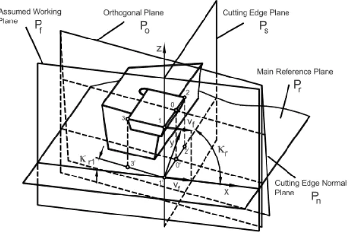
The cutting tool geometry includes a number of angles measured in different planes [3]. Figure 2.3 visualizes the definition of the main reference plane Pr as

perpendicular to the assumed direction of primary motion (the z-direction in Fig-ure 2.3). This figFig-ure also sets the tool-in-hand coordinate system. In this figFig-ure,

f

v is the assumed direction of the cutting feed, line 12 is the major cutting edge and 13 is the minor cutting edge. The tool-in-hand system consists of five basic planes defined relative to the reference plane Pr [4], some of which are illustrated

in Figure 2.3:

• Perpendicular to the reference plane Pr and containing the assumed

direc-tion of feed modirec-tion is the assumed working plane Pf

• The tool cutting edge plane Ps is perpendicular to Pr, and contains the

ma-jor cutting edge (1–2 in Figure 2.3)

v_f v_f x y z κ_r Pr 1 3 2 I I I 3 ₁ 2 κr1

Main Reference Plane

0

0'

Cutting Edge Plane

P_s Orthogonal Plane P_o P Assumed Working Plane f

Cutting Edge Normal Plane _P

n

• The tool back plane Pp (not shown) is conicident with the zy-plane and thus

is perpendicular to Pr and Pf

• Perpendicular to the projection of the cutting edge into the reference plane is the orthogonal plane Po (in Figure 2.3 shown as passing thorugh the

point 0’ selected on the projection of the cutting edge)

• The cutting edge normal plane Pn is perpendicular to the cutting edge

The geometry of the cutting tool is defined by a set of the basic tool angles in the corresponding reference planes shown in Figure 2.3. The definitions of basic tool angles in the tool-in-hand system are as follows:

• Ψis the tool approach angle; it is the acute angle that Ps makes with Pp and

is measured in the reference plane as shown in Figure 2.4;

• The rake angle is the angle between the reference plane (the trace of which in the considered plane of measurement appears as the normal to the direction of primary motion) and the intersection line formed by the considered plane of measurement and the tool rake plane. The rake angle is defined as always being acute and positive when looking across the rake face from the selected point and along the line of intersection of the

αn n β γn SECTION N-N (Plane P ) n λs −λ +λ r P (Plane P ) VIEW S s p α βp p γ P_r SECTION P-P (Plane P )_p N N P_f (Plane P ) αo βo o SECTION O-O γo s P s P r P F O P P F O (Plane P ) SECTION F-F f P_r P_p αf f γ βf S −γ +γ κr ψr κr1 2 0 1 3 O' SECTION O'-O' (Plane O') 1o α O'

face and plane of measurement. The viewed line of intersection lies on the opposite side of the tool reference plane from the direction of primary motion in the measurement plane for γf, γp, γo or a major component of it

appears in the normal plane for γn. The sign of the rake angles is well

de-fined (Figure 2.4).

• The flank angles are defined in a way similar to the rake angles, although here, if the viewed line of intersection lies on the opposite side of the cut-ting edge plane Ps from the direction of feed motion (assumed or actual as

the case may be) then the flank angle is positive. Angles αf, αp, αo, and αn

are clearly defined in the corresponding planes as seen in Figure 2.4. The flank (clearance) angle is the angle between the tool cutting edge plane Ps

and the intersection line formed by the tool flank plane and the considered plane of measurement, as shown in Figure 2.4.

• The wedge angles βf, βp, βo and βn are defined in the planes of

measure-ments. The wedge angle is the angle between the two intersection lines formed as the corresponding plane of measurement intersects with the rake and flank planes.

• The orientation and inclination of the cutting edge are specified in the tool cutting edge plane Ps. In this plane, the cutting edge inclination angle λs is

the angle between the cutting edge and the reference plane.

• The definition of the tool cutting edge angle, κr, is shown in Figure 2.2. It

is defined as the acute angle that the tool cutting edge plane makes with the assumed working plane and is measured in the reference plane Pr.

Simi-larly, the tool minor (end) cutting edge angle, κr1, is the acute angle that the

minor cutting edge plane makes with the assumed working plane and is measured in the reference plane Pr.

2.1.5 Influence of the Tool Angles

Thetoolcuttingedgeangle significantly affects the cutting process because, for a given feed and cutting depth, it defines the uncut chip thickness, width of cut, and thus tool life. The physical background of this phenomenon can be explained as follows: when κr decreases, the chip width increases correspondingly because the

active part of the cutting edge increases. This results in improved heat removal from the tool and hence tool life increases. For example, if the tool life of a high-speed steel (HSS) face milling tool having κr=60° is taken to be 100% then when κr=30°

its tool life is 190%, and when κr=10° its tool life is 650%. An even more profound

effect of κr is observed in the machining with single-point cutting tools. For

exam-ple, in rough turning of carbon steels, the change of κr from 45° to 30° sometimes

leads to a fivefold increase in tool life. The reduction of κr, however, has its

draw-backs. One of these is the corresponding increase of the radial component of the cutting force, which reduces the accuracy and stability of machining particularly when the machine, tool holder and workpiece fixture are not suficiently rigid.

Rake angles come in three varieties: positive, zero (sometimes referred to as neutral) and negative, as indicated in Figure 2.4. It is generally accepted that an

increase in the rake angle reduces horsepower consumption per unit volume of the layer being removed at the rate of 1% per degree starting from γ=–20°. As a result, the cutting force and tool–chip contact temperature change in approxi-mately the same way. So, it seems to be reasonable to select a high positive rake angle for practical cutting operations. Everyday machining practice, however, shows that there are number of drawbacks of increasing the rake angle.

The main drawback is that the strength of the cutting wedge decreases when the rake angle increases. When cutting with a positive rake, the normal force on the tool–chip interfaces causes bending of the tip of the cutting wedge. The pres-ence of the bending significantly reduces the strength of the cutting wedge, caus-ing its chippcaus-ing. Moreover, the tool–chip contact area reduces with the rake an-gle so the point of application of the normal force shifts closer to the cutting edge. On the contrary, when cutting with a tool having a negative rake angle, the mentioned normal force causes the compression of the tool material. Because tool materials have very high compressive strength, the strength of the cutting edge in this case is much higher, although the normal force is greater than that for tools with positive rake angles. Another essential drawback is that the region of the maximum contact temperature at the tool–chip interface shifts toward the cutting edge when the rake angle is increased, which lowers tool life as dis-cussed by Astakhov [5].

Realistically, the rake angle is not an independent variable in the process of tool geometry selection because the effect of the rake angle depends upon other pa-rameters of the cutting tool geometry and the cutting process. Moreover, the ne-cessity of applying chip breakers of different shapes often dictates the resulting rake angle rather than other parameters of the cutting process such as tool life, power consumption and cutting force.

Flank angle. If the flank angle α=0° then the flank surface of the cutting tool is in full contact with the workpiece. As such, due to spring-back of the workpiece material, there is a significant friction force in such a contact that usually leads to tool breakage. The flank angle affects the performance of the cutting tool mainly by decreasing the rubbing on the tool’s flank surfaces. When the uncut chip thick-ness is small (less than 0.02 mm), this angle should be in the range 30–35° to achieve maximum tool life.

The flank angle directly affects tool life. When the angle α increases, the wedge angle β decreases, as seen in Figure 2.4. As such, the strength of the region adjacent to the cutting edge decreases as well as the heat dissipation through the tool. These factors lower tool life. On the other hand, the following advantages may be gained by increasing the flank angle: (a) the cutting edge radius decreases with the flank angle, which leads to corresponding decreases in the frictional and deformation components of the flank force. This effect becomes noticeable in cutting with small feeds. As a result, less heat is generated, which leads to an in-crease in tool life, (b) as the flank angle becomes larger, more tool material has to be removed (worn out) to reach the same flank wear VB, increasing tool life. As a result of such contrary effects, the influence of the flank angle on tool life al-ways has a well-defined maximum. In other word, there is alal-ways an optimal flank angle that should be found for a given machining operation.

Inclination angle. The sense and sign of the inclination angle λs is clearly

shown in Figure 2.4 and is defined earlier as the angle between the cutting edge and the reference plane; experience shows that there are certain difficulties and confusions in understanding this angle. When the angle λs is positive, the chip

flows to the right and when it is negative the chip flows to the left. The direction of chip flow, however, is defined not only by the angle λs but also by the cutting

edge angle κr.

2.2 Tool

Materials

Many types of tool materials, ranging from high-carbon steels to ceramics and diamonds, are used as cutting tool materials in today’s metalworking industry. It is important to be aware that differences exist among tool materials, what these dif-ferences are and the correct application for each type of material [6].

The three prime properties of a tool material are:

• Hardness: defined as the resistance to indenter penetration. It is directly correlates with the strength of the cutting tool material [7]. The ability to maintain high hardness at elevated temperatures is called hot hardness. Figure 2.5 shows the hardness of typical tool materials as a function of temperature.

• Toughness: defined as the ability of a material to absorb energy before fracture. The greater the fracture toughness of a tool material, the better it resists shock load, chipping and fracturing, vibration, misalignments, runouts and other imperfections in the machining system. Figure 2.6 shows

50 300 500 700 900 1100 70 90 Temperature, o_C Har dne s s HR C

Carbon Tool Steels

HSS

Carbides PCD

Ceramics

that, for tool materials, hardness and toughness change in opposite direc-tions. A major trend in the development of tool materials is to increase their toughness while maintaining hardness.

• Wear resistance: In general, wear resistance is defined as the attainment of acceptable tool life before tools need to be replaced. Although seem-ingly very simple, this characteristic is the least understood.

Wear resistance is not a defined characteristic of the tool material and the meth-odology of its measurement. The nature of tool wear, unfortunately, is not yet sufficiently clear despite numerous theoretical and experimental studies. Cutting tool wear is a result of complicated physical, chemical, and thermo-mechanical phenomena. Because various simple mechanisms of wear (adhesion, abrasion, diffusion, oxidation etc.) act simultaneously with a predominant influence of one or more of them in different situations, identification of the dominant mecha-nism is far from simple, and most interpretations are subject to controversy. As the most common experimental device used by hard tool material manufacturers to characterize wear resistance is a pin-on-disk tribometer. The unacceptability of this method and thus the obtained results were discussed by Astakhov [5]. The toughness of a hard tool material is an even less relevant characteristic bearing in mind the methods used in its determination. For carbides, the

short-rod fracture toughness measurement is common, as described in the ASTM

standard B771-87. The test procedure involves testing of chevron-slotted speci-mens and recording the loading. As shown by Astakhov (page 150, Figure 4.8 in [4]), fracture toughness can vary by 300% depending on the loading conditions (stress state, strain rate and temperature). Therefore, the toughness of the tool materials should be determined using loading conditions similar to that occurred in machining. HA RDN E S S TOUGHNESS Cobalt HSS PCD DLC PCBN HSS PM HSS Ceramics Al2O3 Si3N4 _{Coated Cermet} Cermet Coated Carbide

Carbide Micrograin Carbide

Coated Micrograin Carbide

Although a number of different tool materials are available today, five most important groups will be outlined in this section: carbides, ceramics, polycrystal-line cubic boron nitrides (PCBNs), polycrystalpolycrystal-line diamonds (PCDs) and solid or thick film diamond (SFDs or TFDs).

2.2.1 Carbides

Carbide as a tool material was discovered in the search for a replacement for ex-pensive diamond dies used in the wire drawing of tungsten filaments. Initiated by a shortage of industrial diamonds at the beginning of World War I, researchers in Germany had to look for alternatives. On 10 June 1926 the name WIDIA (from the German term Wie Diamant, i.e., like diamond) was entered into the register of trademarks and an arduous period of work started to transform laboratory-scale experiments into industrial production. The first product (Widia N – WC-6Co) was presented at the Leipzig Spring Fair in 1927.

2.2.1.1 Composition

Today, carbide tool materials include silicon and titanium carbides (called cerments) and tungsten carbides and titanium carbides as well as other compounds of a metal (Ti, W, Cr, Zr) or metalloid (B, Si) and carbon. Carbides have excellent wear resis-tance and high hot hardness. The terms tungstencarbide and sinteredcarbide for a tool material describe a comprehensive family of hard carbide composits used for metal cutting tools, dies of various types and wear parts [8]. A carbide tool material consists of carbide particales (carbides of tungsten, titanium, tantalum or some com-bination of these) bound together in a cobalt matrix by sintering. Normally, the size of the carbide particles is less than 0.8 μm for micrograins, 0.8–1.0 μm for fine grains, 1–4 μm for medium grains, and more than 4 μm for coarse-grain cutting in-serts. The amount of cobal significantly affects the properties of carbide inin-serts. Normally, the cobalt content is 3–20%, depending upon the desired combination of toughness and hardness. As the cobalt content increases, the toughness of a cuting insert increases while its hardness and strength decrease. However, the correct com-bination of carbide insert composition (grade), coating materials, layer sequence and the selection of the appropriate coating technology makes it possible to increase metal cutting productivity substantially without sacrificing insert wear resistance. 2.2.1.2 Selection

The selection of the most advantageous carbide grade has become as sophisticated a factor as the design of the tooling itself. A wide variety of new carbide grades and coatings available today continue to complicate the manufacturing engineer’s task of selecting the optimum grade as it relates to work material machinability, hardness and desired productivity, efficiency and quality. Coupled with newer, high-speed, powerful machines and coolant brands and supply techniques, this selection have created a real cutting tool insert selection dilemma for many spe-cialists in the field. Because many manufacturing facilities do not have the luxury

of a machining laboratory or even the time to carry out machining evaluations for different cutting parameters, cutting tool manufacturers offer a guide for the initial selection, as shown in Table 2.1.

2.2.1.3 Coating

One of the most revolutionary changes in the metal cutting industry over the last 30 years has been thin-film hard coatings and thermal diffusion processes. These methods find ever-increasing applications and brought significant advantages to their users. Today, 50% of HSS, 85% of carbide and 40% of super-hard tools used in industry are coated [5]. A great number of coating materials, methods and re-gimes of application on substrates or whole tools and multi-layer coating combina-tions are used.

Table 2.1. Guides to select carbide grade for a given application

Cutting conditions Code Colour

Finishing steels, high cutting speeds, light cutting feeds,

favourable work conditions P01

Finishing and light roughing of steels and castings

with no coolant P10

Medium roughing of steels, less favourable conditions.

Moderate cutting speeds and feeds. P20

General-purpose turning of steels and castings,

medium roughing P30

Heavy roughing of steels and castings,

intermittent cutting, low cutting speeds and feeds P40 Difficult conditions, heavy roughing/intermittent

cutting, low cutting speeds and feeds P50

Blue

Finishing stainless steels at high cutting speeds M10 Finishing and medium roughing of alloy steels M20 Light to heavy roughing of stainless steel

and difficult-to-cut materials M30

Roughing tough skinned materials

at low cutting speeds M40

Yellow

Finishing plastics and cast irons K01

Finishing brass and bronze at high cutting speeds

and feeds K10

Roughing cast irons, intermittent cutting,

low speeds and high feeds K20

Roughing and finishing cast irons and non-ferrous

materials. Favourable conditions K30

Carbides are excellent substrates for all coatings such as TiN, TiAlN, TiCN, solid lubricant coatings and multilayer coatings. Coatings considerably improve tool life and boost the performance of carbide tools in productivity, high-speed and high-feed cutting or in dry machining, and when machining of difficult-to-machine materials. Coatings: (a) provide increased surface hardness, for greater wear, (b) increase resistance (abrasive and adhesive wear, flank or crater wear), (c) reduce friction coefficients to ease chip sliding, reduce cutting forces, prevent adhesion to the contact surfaces, reduce heat generated due to chip sliding etc., (d) reduce the portion of the thermal energy that flows into the tool, (e) increase cor-rosion and oxidation resistance, (f) improve crater wear resistance and (g) im-proved the surface quality of finished parts.

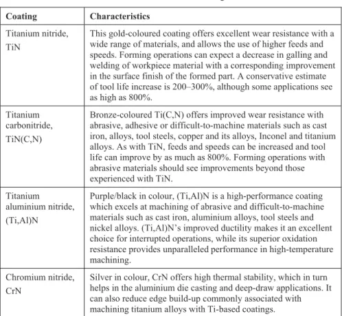
Common coatings for carbides applied in single- or multi-layers are shown in Figure 2.7. They are:

• TiN: general-purpose coating for improved abrasion resistance. Colour – gold, hardness HV (0.05) – 2300, friction coeficient – 0.3, thermal stabil-ity – 600°C.

• TiCN: multi-purpose coating intended for steel machining. Higher wear re-sistance than TiN. Available in mono- and multi-layer. Colour – grey-violet, hardness HV (0.05) – 3000, friction coeficient – 0.4, thermal stabil-ity – 750°C.

• TiAlN and TiAlCN – High-performance coating for increased cutting pa-rameters and higher tool life; also suitable for dry machining. Reduces heating of the tool. Multi-layered, nanostructured or alloyed versions offer even better performance. Colour – black-violet, hardness HV (0.05) – 3000–3500, friction coeficient – 0.45, thermal stability – 800–900°C.

Substrate Substrate Substrate Substrate Substrate

TiN TiC TiCN TiN TiN TiAlN WC/C TiAlN Monolayer Gradient layer

Maltilayers Nanolayers Hard/soft layers Figure 2.7. Modern coatings

• WC-C and MoS2 – Provides solid lubrication at the tool–chip interface that

significantly reduces heat due to friction. Has limited temperaure resis-tance. Recommended for high-adhesive work materials such as aluminium and copper alloys and also for non-metallic materials. Colour – gray-black, hardness HV (0.05) – 1000–3000, friction coeficient – 0.1, thermal stabil-ity – 300°C.

• CrN – Intended for copper alloys such as brass, bronze etc. Colour – metallic. Coating fracture toughness is as important as coating hardness in crack retarda-tion. Balance between high compressive stress (poor adhesion) and low residual stress (no crack retardation) is necessary.

A great attempt to correlate the counting materials and their performance was made by Klocke and Krieg [9]. It was pointed out that there are basically four major groups of coating materials on the market. The most popular group is titanium-based coating materials as TiN, TiC and Ti(C,N). The metallic phase is often sup-plemented by other metals such as Al and Cr, which are added to improve particular properties such as hardness or oxidation resistance. The second group represents ceramic-type coatings as Al2O3 (alumina oxide). The third group includes

super-Table 2.2. Basic PVD coatings Coating Characteristics Titanium nitride,

TiN

This gold-coloured coating offers excellent wear resistance with a wide range of materials, and allows the use of higher feeds and speeds. Forming operations can expect a decrease in galling and welding of workpiece material with a corresponding improvement in the surface finish of the formed part. A conservative estimate of tool life increase is 200–300%, although some applications see as high as 800%.

Titanium carbonitride, TiN(C,N)

Bronze-coloured Ti(C,N) offers improved wear resistance with abrasive, adhesive or difficult-to-machine materials such as cast iron, alloys, tool steels, copper and its alloys, Inconel and titanium alloys. As with TiN, feeds and speeds can be increased and tool life can improve by as much as 800%. Forming operations with abrasive materials should see improvements beyond those experienced with TiN.

Titanium

aluminium nitride, (Ti,Al)N

Purple/black in colour, (Ti,Al)N is a high-performance coating which excels at machining of abrasive and difficult-to-machine materials such as cast iron, aluminium alloys, tool steels and nickel alloys. (Ti,Al)N’s improved ductility makes it an excellent choice for interrupted operations, while its superior oxidation resistance provides unparalleled performance in high-temperature machining.

Chromium nitride, CrN

Silver in colour, CrN offers high thermal stability, which in turn helps in the aluminium die casting and deep-draw applications. It can also reduce edge build-up commonly associated with machining titanium alloys with Ti-based coatings.

hard coatings, such as chemical vapor deposition (CVD) diamond. The fourth group includes solid lubricant coating such as amorphous metal-carbon. Additionally, to reduce extensive tool wear during cut-in periods, some soft coatings as MoS2 or

pure graphite are deposited on top of these hard coatings. The basic physical vapor deposition (PVD) coatings are listed in Table 2.2. The effectiveness of various coatings on cutting tools is discussed by Bushman and Gupta [10].

2.2.2 Ceramics

Introduced in the earlier 1950s, ceramic tool materials consist primarily of fine-grained aluminium oxide, cold-pressed into insert shapes and sintered under high pressure and temperature. Pure alumimum oxide ceramics are called white ceram-ics while the addition of titanium carbide and zirconiou oxide results in black cermets (not to be confuse with the carbide cermets discussed earlier).

The prime benefit of ceramics is high hardness (and thus abrasive wear resis-tance) at elevated temperatures, as seen in Figure 2.6. All tool materials soften as they become hotter, but ceramics do so at a much slower rate because they are not metal limited. Among the major advantages of ceramic cutting tools is also chem-ical stability. In practchem-ical terms this means that the ceramic does not react with the material it is cutting, i.e., there is no diffusion wear, which is the weakest spot of carbides in high-speed machining applications.

Ceramics are suitable for machining the majority of ferrous materials, including superalloys. It should not be used, however, for copper, brass and aluminium due to the formation of an excessive built-up edge. There are indications that alumin-ium-oxide-based ceramics are being replaced by PCBN. PCBN is taking over much of the ceramic work because it works better for softer materials.

The downside to these ceramic materials is a slightly higher cost and brittleness. To protect their cutting edges, ceramics are typically made with a heavy edge prepa-ration such as a T-land or honed edge or with modern edge prepaprepa-ration features.

There are two basic kinds of ceramics. The first is aluminium oxide. It is wear-resistant but brittle, and used chiefly on hardened steel. The other major type is silicon nitride, which is relatively soft and tough and is used on cast irons. Between aluminium oxide and silicon nitride fall a whole host of ceramic mate-rials called Si-AlONs that combine the two. The greater the proportion of alu-minium oxide, the harder the material. The more silicon nitride included, the tougher the material.

In the leap-frog race between work materials and tools, the laurels still go to the tools. The cutting ability of the tool is still slightly ahead of the applications (in-cluding available machine tools and their relevant characteristics) because there is a reluctance to apply the available cutting tool technology. However, when one moves to high-speed machining, one has to make major changes to the existing machining operation, including fixturing, chucks, guards, programming, coolants and a lot of other housekeeping issues. Not everyone wants to take the trouble, or spend the money, to do this. In making the ultimate decision, lot size determines to a large extent whether high speed, and therefore ceramics, is practical.

It was a little disappointed that ceramic-reinforcement technology has not moved ahead as quickly as initially supposed. Reinforcements offer a lot of strength

advantages. They are available, but not in widespread use. It now seems that a new area that will offer a lot of new advantages in ceramic tools is nanotechnology. The most advanced ceramics today are micrograin materials, while the latest de-velopments aim to move to nanograins or particle sizes of less than a micron. This technology is coming along well. The main advantage it offers is that the smaller particle size increases strength because more grain area is exposed to bonding. This strength increase translates into greater impact resistance and improved wear properties.

Coatings are rarely used with ceramic inserts. On ceramics, coatings do some good but the cost is high and usually does not justify the end result, because of weak adhesion between the coating materials and ceramic substrate.

For ceramics, the future is bright because of the push for high-speed machining. Modern machines now typically operate in the 600–900 m/min range while speeds of 1500 m/min are being tested. Only advanced cutting-tool materials can handle this speed. There has been a lot of improvement in wear, chiefly through the adoption of small grain sizes. For example, in hard turning applications with ceramics, tool life is improved up to 20-fold with modern grades. Cermets are a slow-growth product in many countries except Japan, where part manufacturing starts with a blank that is near net shape, which in many cases requires just finishing with cermets.

2.2.3 Cubic Boron Nitride (CBN)

Polycrystalline CBN blanks are manufactured from cubic boron nitride crystals utilizing an advanced high-temperature, high-pressure process. The cubic boron nitride crystals are sintered together with a binder phase and integrally bonded to a tungsten carbide substrate. The binder phase, usually either a metallic or ceramic matrix, provides chemical stability, enabling the PCBN qualities to be utilized in high-speed machining environments. The tungsten carbide substrate in the PCBN blanks provides the high impact resistance necessary for the depths of cuts and high speeds associated with machining of hardened ferrous materials. PCBN cut-ting tools offer excellent heat dissipation and wear resistance. Cutcut-ting tool geome-tries can be prepared to withstand interrupted cuts with a T-land and/or honed to stabilize the cutting edge and prolong tool life.

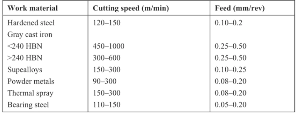
PCBN tools offer the following benefits: (a) machine-hardened and heat-treated steels, (b) an excellent surface finish that allows eliminate grinding, (c) high pro-ductivity rate that can be more than four times higher than that in grinding, (d) great resistance to abrasion which is twice that of ceramics and ten times than that of carbide. PCBN tools are recommended for machining cast irons including com-pacted graphite iron (CGI), sintered iron and superalloys hardened steels. Typical machining regimes are shown in Table 2.3.

To promote good tool life, the cutting edge of the PCBN insert must be rein-forced with proper edge preparation. This can range from a small hone for finish-machining cast irons, to a T-land measuring 0.2 mm wide by 15° for heavy rough-ing of white iron. Combined lands and hones may also be used. Table 2.4 shows typical parameters of the T-land applied for PCBN inserts.

Users of superhard materials such as PCBN and PCD in cutting tools com-monly believe that chamfering, also known as applying a T-land or K-land, is

Table 2.4. Edge preparation parameters for PCBN inserts Work

material Roughning Finishing

Hardened steel fch=0.2–0.5, γch=20°

fch=0.2, γch=20°

Gray cast iron fch=0.2, γch=15–20°

Hone r=0.2 Hard cast iron fch=0.2–0.5,

γch=15–20° fch=0.2, γch=20° Powder metal fch=0.2, γch=20° fch=0.2, γch=20° Superalloys fch=0.2–0.5, γch=20°

necessary for extending tool life. This practice is so widely accepted that many industry professionals have never even seen a CBN cutting tool without a chamfer; and they assume that it is a necessary feature of the tool. In fact, chamfering, in most cutting tool applications, has been proven to be a sub-optimal solution that limits tool life and diminishes cutting performance. With the advent of advanced edge preparation technology and edge preparation machines, alternatives to chamfering now exist so chamfering is no longer a necessity for CBN and PCD cutting tools.

2.2.4 Polycrystalline Diamond (PCD)and Solid Film Diamond (SFD)

Being the most southt-after gemstone in the world, diamond may well also be the world’s most versatile engineering material. Diamond is the strongest and hardest known substrate, it has the highest thermal conductivity of any material at room temperature, low-friction surface and optical transparancy. This unique combina-tion of properties cannot be matched by any other material [11].

Table 2.3. Typical machining regimes for CBN

Work material Cutting speed (m/min) Feed (mm/rev) Hardened steel

Gray cast iron <240 HBN >240 HBN Supealloys Powder metals Thermal spray Bearing steel 120–150 450–1000 300–600 150–300 90–300 150–300 110–150 0.10–0.2 0.25–0.50 0.25–0.50 0.10–0.25 0.08–0.20 0.08–0.20 0.05–0.20 ch ch γ CBN Carbide

To produce PCD used in cutting tools, a layer of diamond crystals, made out of a mixture of graphite and a catalyst (typically nickel) under a pressure of approxi-mately 7000 MPa and temperature of 1800°C, is placed on a carbide substrate and subjected to a high-temperature high-pressure process (6000 MPa, 1400°C). Dur-ing this process, cobalt from the tungsten substrates becomes the binder of the diamond crystals giving polycrystalline diamond the required toughness.

PCD tool materials typically provide abrasion resistance up to 500 times that of tungsten carbide and high thermal conductivity. PCD tools have replaced tungsten carbide, ceramics and natural diamond in a range of high-performance applications including the turning, boring, milling, slotting and chamfering of materials such as high-silicon aluminium, metal matrix composites (MMC), ceramics, reinforced epoxies, plastics, carbon-fibre-reinforced plastics (CFRP) and engineered wood products. The extended tool life and increased productivity provided by PCD tools often offset the higher initial cost by lowering the unit cost of parts produced. Use-ful tool life may be further extended through multiple re-sharpenings. Table 2.5 shows typical machining regimes for PCD tools.

Selecting the optimum grade of PCD tooling for a specific application is gen-erally a function of surface finish requirements and tool life expectations. Mate-rial removal rates, tool geometries and mateMate-rial characteristics also affect the relationship between machining productivity, tool life and surface finish. Coarse-grade PCD is designed with a larger diamond particle size than a fine-Coarse-grade PCD. Generally, PCD with larger diamond particles exhibits greater abrasion resistance, but results in a rougher cutting edge. Conversely, smaller diamond particle will result in a sharper cutting edge, producing a superior workpiece surface finish, but tool life is reduced.

Having high abrasion resistance and great hardness, PCDs suffer from rela-tively low toughness. To overcome this shortcoming, the development of new prime grades of PCDs relies on structural changes that enhance toughness. One of the most promising directions is to combine diamond particle of different sizes (for example, 30 and 2 μm, as proposed by Element 6 Co.) in the mixture to in-crease the diamond packing density, as shown in Figure 2.8. The improved pack-ing density results in a higher degree of contiguity between diamond grains, thereby enhancing resistance to chipping of the cutting edge. An added advantage of the increased packing density is the quality of the ground cutting edge as the filling of the area between the coarse diamond grains with fine diamond yields a continuous as opposed to the micro-serrated irregular cutting edge obtained with usual PCD grades.

Thick-film diamond (TFd) tools constitute a major breakthrough in the science of cutting tools. The company SP3 has been developing thick-film diamond tech-nology for several years, and now offers a new product line of TFd cutting tools. A stand-alone sheet of thick-film diamond is grown in a chemical vapour deposi-tion reactor. Typical films are 500 μm thick and come in flat sheets. These sheets are than laser cut into tips, which are secured into tool bodies using a specially developed brazing process. Axial end tools such as as drills, reamers, boring tips, cartridges for boring bars and milling tools are produced. Application-specific tool

design with TFd is now under extensive development at the most advanced auto-motive manufacturing power-train facilities.

TFd provides three distinct advantages over PCD tools: (a) it is intrinsically harder and more wear resistant than PCD because it is solid diamond with no binder material; (b) when machining abrasive metals with TFd, the tool wears primarily on the flank. This causes the cutting edge to remain sharper than PCD as the tool wears. This is particularly imeportant in applications where burr control is crucial to producing good parts. The life of TFd tools is depend-ent on edge recession and is not limited by premature failure related to edge sharpness; and (c) There is no possibility of chemical interaction with the cool-ant or by-products of the workpiece material because there is no binder in TFd. As a result, the tool life of TFd tools is substantially longer than that of PCD tools (Figure 2.9).

Thick-film diamond tools have demonstrated tool life two to three times that of PCD tools in tests conducted by an independent test laboratory. Thick-film diamond tools are the first to evidence performance exceeding that of PCD in 25 years. 0 2 4 6 8 PCD CFd 1.00 1.98 2.75 6.17 Dry Wet Relat

ive Tool Life

Figure 2.9. Relative performance of TFd versus PCD in turning of high-silicon aluminium alloy 390 (up to 18% Si)

Figure 2.8. Improving packing density by combining diamonds of considerably different sizes

Table 2.5. Recommended machining regimes Work material Cutting speed

(m/min) Cutting feed (mm/rev) Depth of cut (mm) Aluminium alloys <12% Si >12% Si 1000–3000 200–600 0.1–0.4 0.1–0.4 5 1 Metal matrix composites

(MMC) 150–600 0.1–0.4 0.5

Brass 600–2000 0.1–0.4 1.5

Hard plastics 1000–7000 0.1–0.7 2.5

Carbon-fibre-reinforced

plastics (CFRP) 500–2000 0.05–0.4 4

Sintered tungsten carbide

18% Co 40–60 0.05–0.2 0.5

Precious metals 100–500 0.05–0.4 1.5

2.3 Tool

Wear

Tool wear leads to tool failure. According to many authors, the failure of cutting tool occurs as premature tool failure (i.e., tool breakage) and progressive tool wear. Figure 2.10 shows some types of failures and wear on cutting tools.

Generally, wear of cutting tools depends on tool material and geometry, work-piece materials, cutting parameters (cutting speed, feed rate and depth of cut), cutting fluids and machine-tool characteristics.

2.3.1 Tool Wear Types

Normally, tool wear is a gradual process. There are two basics zones of wear in cutting tools: flank wear and crater wear.

Flank and crater wear are the most important measured forms of tool wear. Flank wear is most commonly used for wear monitoring. According to the stan-dard ISO 3685:1993 for wear measurements, the major cutting edge is considered to be divided in to four regions, as shown in Figure 2.11:

• Region C is the curved part of the cutting edge at the tool corner; • Region B isthe remaining straight part of the cutting edge in zone C;

• Region A is the quarter of the worn cutting edge length b farthest away

• Region N extends beyond the area of mutual contact between the tool workpiece for approximately 1–2 mm along the major cutting edge. The wear is of notch type.

The width of the flank wear land, VBB, is measured within zone B in the cutting

edge plane Ps (Figures 2.3 and 2.11) perpendicular to the major cutting edge. The

width of the flank wear land is measured from the position of the original major cutting edge.

The crater depth, KT, is measured as the maximum distance between the crater bottom and the original face in region B.

Tool wear is most commonly measured using a toolmaker’s microscope (with video imaging systems and a resolution of less than 0.001 mm) or stylus instru-ment similar to a profilometer (with ground diamond styluses).

2.3.2 Tool Wear Evolution

Tool wear curves illustrate the relationship between the amount of flank (rake) wear and the cutting time, τm, or the overall length of the cutting path, L.

Fig-ure 2.12(a) shows the evolution of flank wear VBB max, as measured after a

cer-tain length of cutting path. Normally, there are three distinctive regions that can be observed in such curves. The first region (region I in Figure 2.12(a)) is the region of primary or initial wear. The relatively high wear rate (an increase of tool wear per unit time or length of the cutting path) in this region is explained by accelerated wear of the tool layers damaged during manufacturing or re-sharpen-ing. The second region (region II in Figure 2.12(a)) is the region of steady-state wear. This is the normal operating region for the cutting tool. The third region (region III in Figure 2.12(a)) is known as the tertiary or accelerated wear region. Accelerated tool wear in this region is usually accompanied by high cutting forces, temperatures and severe tool vibrations. Normally, the tool should not be used in this region.

In practice, the cutting speed is of prime concern in the consideration of tool wear. As such, tool wear curves are constructed for different cutting speeds keep-ing other machinkeep-ing parameters constant. In Figure 2.12(b), three characteristic tool wear curves (mean values) are shown for three different cutting speeds, v1,

VBB VB_N VB max._B N B C VB_C Flank wear land Zone A SECTION A-A Crater s Plane P KM KB KT b A KF

KF = crater front distance KB = crater width

KM = crater center distance KT = crater depth

Notch wear

2

v , and v3. Because v3 is greater than the other two, it corresponds to the fastest

wear rate. When the amount of wear reaches the permissible tool wear VBBc, the

tool is said to be worn out.

Typically VBBc is selected from the range 0.15–1.00 mm depending upon the

type of machining operation, the condition of the machine tool and the quality requirements of the operation. It is often selected on the grounds of process effi-ciency and often called the criterion of tool life. In Figure 2.12(b), T1 is the tool

life when the cutting speed v1 is used, T2 – when v2, and T3 – when v3is the

case. When the integrity of the machined surface permits, the curve of maximum wear instead of the line of equal wear should be used (Figure 2.12(b)). As such, the spread in tool life between lower and higher cutting speeds becomes less sig-nificant. As a result, a higher productivity rate can be achieved, which is particu-larly important when high-speed CNC machines are used.

Figure 2.13 shows an example of typical flank wear of a CVD diamond tool, which can be observed during machining of a high-silicon aluminium alloy (MMC).

The criteria recommended by ISO3685:1993 [13] to define the effective tool life for cemented carbides tools, high-speed steels (HSS) and ceramics are:

Cemented carbides: 1. VBB=0.3 mm, or

2. VBB,max=0.6 mm, if the flank is irregularly worn, or;

3. KT=0.06+0.3 f, where f is the feed. HSS and ceramics:

1. Catastrophic failure, or;

2. VBB=0.3 mm, if the flank is regularly in region B; or

3. VBB,max=0.6mm, if the flank is irregularly in region B. 1000 0 500 1500 2000 0.25 0.50 0.75 1.00 (m) 3000 2500 L (a) I II III max (mm)B VB 1 2 3 (b) V Curve of maximum wear T₃ 0 0 Bc VB 3 1 T T₂ τ _m Line of equal wear 2 1 4 1 B VB V < V < V V 2 V 5 3 1 2 3

Figure 2.12. Wear curves: (a) normal wear curve, (b) evolution of flank wear land VBB as a function of cutting time for different cutting speeds

Figure 2.13. Example of flank wear for CVD diamond tool in machining MMC (Vc= 50 m/min, f=0.2 mm/rev, doc=1mm and cutting time 4.5 min) [14]

Table 2.6. Recommendations used in industrial practice for limit of flank wear VBB for

several cutting materials

Tool material HSS Cemented

carbides Carbides coateds Ceramics Operation (mm) Al2O3 Si3N4 Roughing VBB 0.35–1.0 0.3–0.5 0.3–0.5 0.25–0.3 0.25–0.5 Finishing VBB 0.2–0.3 0.1–0.25 0.1–0.25 0.1–0.2 0.1–0.2

General recommendations used in industrial practice for the limit of

flank wear VBB for several cutting materials are given in Table 2.6.

2.3.4 Mechanisms of Tool Wear

The general mechanisms that cause tool wear, summarized in Figure 2.14, are: (1) abrasion, (2) diffusion, (3) oxidation, (4) fatigue and (5) adhesion. The fundaments of there tool wear mechanisms are explained for several authors, for example, Shaw [15] and Trent and Wright [16]. Most of these mechanisms are accelerated at higher cutting speeds and consequently cutting temperatures.

2.4 Tool

Life

Tool life is important in machining since considerable time is lost whenever a tool is replaced and reset. Tool life is the time a tool will cut satisfactorily and is ex-pressed as the minutes between changes of the cutting tool. The process of wear

and failures of cutting tools increases the surface roughness, and the accuracy of workpieces deteriorates.

2.4.1 Taylor’s Tool Life Formula

Tool wear is almost always used as a lifetime criterion because it is easy to deter-mine quantitatively. The flank wear land VBB is often used as the criterion

be-cause of its influence on workpiece surface roughness and accuracy. Figure 2.15 shows the wear curves (VBB versus cutting time) for several cutting velocities (1,

2 and 3) and the construction of the life curve (cutting velocity versus tool life). Taylor [17] presented the following equation:

=

n c

V T C _(2.1)

where Vc is the cutting speed (m/min), T is the tool life (min) taken to develop a

certain flank wear (VBB), n is an exponent that depends on the cutting parameters

and C is a constant. Note that C is equal to the cutting speed at T=1 min.

Therefore, each combination of tool material and workpiece and each cutting parameter has it is own n and C values, to be determined experimentally. For ex-ample, choosing two extreme points (Figure 2.15(a)), points 1 and 3, Vc=200

m/min, T=40 min and Vc=400 m/min and T=10 min, respectively, we have:

200 40× n=_{C (2.2)}

400 10× n=_C

(2.3) Figure 2.14. Evolution of the flank wear land VBB as a function of cutting time for

Figure 2.15. Wear curves for several cutting speeds (1, 2 and 3) (a) and life curve (b) Taking natural logarithms of each term gives

200+ 40= 400+ 10 ln n ln ln n ln _(2.4) 5 298. + ×n 3 689 5 991. = . + ×n 2 303. _(2.5) 0 5 = n . _(2.6)

Substituting this value of n into Equations (2.2) and (2.3), one can calculate the corresponding values of C 0 5 200 40 804 = × . = C _{or C=400 10×} 0 5. _{=1264 9.} (2.7) The Taylor equation for the data show in Figure 2.15 is:

0 5. _{=1264 9} c

V T . _(2.8)

Table 2.7 presents the range of n values determined in practice for some tool materials.

Table 2.7. Values of n observed in practice for several cutting tool materials

Tool material HSS Cemented

carbides Ceramics n 0.1–0.2 0.2–0.5 0.5–0.7 F lan k wea r VB B C uttin g S pe ed V c

Cutting time (min) Tool life (min)

VBBlimit 1 2 3 1 2 3 (a) (b) Vc3 > Vc2> Vc1

2.4.2 Expanded Taylor’s Tool Life Formula

According to the original Taylor tool life formula, the cutting speed is the only parameter that affects tool life. This is because this formula was obtained using high-carbon and high-speed steels as tool materials. With the further development of carbides and other tool materilas, it was found that the cutting feed and the depth of cut are also significant. As a result, the Taylor’s tool life formula was modified to accommodate these changes as:

=

n a b c

V T f d C _(2.9)

where d is the depth of cut (mm) and f is the feed (mm/rev). The exponents a and b are to be determined experimentally for each combination of the cutting condi-tions. In practice, typical values for HSS tools are n=0.17, a=0.77 and b=0.37 [18]. According to this information, the order of importance of the parameters is: cutting speed, then feed, then depth of cut. Using this parameters, Equation (2.9) for the expanded Taylor tool life formula model can be rewritten as:

1 −1 − −

=

a b n _cn n n

T C V f d or _{T C=} 5 88. _V−5 88. _f−4 53. _d−2 18. _(2.10)

Although cutting speed is the most important cutting parameter in the tool life equation, the cutting feed and the depth of cut can also be the significant factors.

Finally, the tool life depends on the tool (material and geometry); the cutting parameters (cutting speed, feed, depth of cut); the brand and conditions of the cutting fluid used; the work material (chemical composition, hardness, strength, toughness, homogenity and inclusions); the machining operation (turning, drilling, milling), the machine tool (for example, stiffness, runout and maintanace) and other machining parameters. As a result, it is nearly impossible to develop a uni-versal tool life criterion.

2.4.3 Recent Trends in Tool Life Evaluation

Although Taylor’s tool life formula is still in wide use today and lies at the very core of many studies on metal cutting, including at the level of national and inter-national standards, one should remember that it was introduced in 1907 as a gen-eralization of many years of experimental studies conducted in the 19th _century

using work and tool materials and experimental technique available at that time. Since then, each of these three components has undergone dramatic charges. Un-fortunately, the validity of the formula has never been verified for these new con-ditions. Nobody has yet proved that it continues to be valid for cutting tool materi-als other than carbon steels and high-speed steels.

Moreover, one should clearly realize that tool life is not an absolute concept but depends on what is selected as the tool life criteria. In finishing operations, surface integrity and dimensional accuracy are of primary concern, while in rough-ing operations the excessive cuttrough-ing force and chatter are limitrough-ing factors. In both

applications, material removal rate and chip breaking could be critical factors. These criteria, while important from the operational point of view, have little to do with the physical conditions of the cutting tool.

To analyze the performance of cutting tools on CNC machines, production cells and manufacturing lines, the dimension tool life is understood to be the time pe-riod within which the cutting tool assures the required dimensional accuracy and required surface integrity of the machined parts.

Although there are a number of representations of the dimension tool life, three of them are the most adequate [5]:

• The dimension wear rate is the rate of shortening of the cutting tip in the direction perpendicular to the machined surface taken within the normal wear period (region II in Figure 2.12(a)), i.e.,

1000 100 − − − = = = = − r r r i l r s h i dv h h vh vfh v dT T T

(

)

where hr and hr i− are the current and initial radial wear, respectively, T and Ti are the total and initial operating time, respectively, and hs is the

surface wear rate. It follows from Equation (2.11) that the dimension wear rate is inversely proportional to the tool life but does not depend on the selected wear criterion (a particular width of the flank wear land, for example).

• Thesurfacewearrate is the radial wear per 1000 cm2 _{of the machined area (S)}

(

)

(

)

(

)

where hr i− and li are the initial radial wear and initial length of the tool

path, respectively, and l is the total length of the tool path. It follows from Equation (2.12) that the surface wear rate is reverse proportional to the overall machined area and, in contrast, does not depend on the selected wear criterion.

• The specific dimension tool life is the area of the workpiece machined by the tool per micron of radial wear

(

)

(

)

(

)

The surface wear rate and the specific dimension tool life are versatile tool wear characteristics because they allow the comparison of different tool materials for different combinations of the cutting speeds and feeds using different criteria se-lected for the assessment of tool life.

References

[1] Rodin PR (1972) The Basics of Shape Formation by Cutting (in Russian). Visha Skola, Kyev (Ukraine)

[2] Granovsky GE, Granovsky VG (1985) Metal Cutting (in Russian), Vishaya Shkola, Moscow

[3] Oxley PLB (1989) Mechanics of Machining: An Analytical Approach to Assessing Machinability. Wiley, New York, NY

[4] Astakhov VP (1998) Metal Cutting Mechanics. CRC, Boca Raton, USA [5] Astakhov VP (2006) Tribology of Metal Cutting. Elsevier: London

[6] Davis JR (Editor) (2005) Tool Materials (ASM Specialty Handbook), ASM Interna-tional, Materials Park, OH, USA

[7] Isakov E (2004) Engineering Formulas for Metalcutting. Industrial, New York, NY [8] Upadbyaya GS (1998) Cemented Tungsten Carbides. Production, Properties, and

Testing. Noyes, Westwood, NJ

[9] Klocke F, Krieg T (1999) Coated tools for metal cutting – features and applications. Ann CIRP 48: 515–525

[10] Bushman B, Gupta BK (1991) Handbook of Tribology-Materials, Coatings, and Surface Treatments. McGraw–Hill, New York, NY

[11] Whitney ED (1994) Ceramic Cutting Tools. Materials, Development, and perform-ance. Noyes, Westwood, NJ

[12] Modern Metal Cutting, A practical Handbook, Sandvik Coromant [13] Tool-life testing with single-point turning tools, ISO 3685:1993

[14] Davim JP (2002) Diamond tool performance in machining metal–matrix composites. J Mater Process Technol 128: 100–105

[15] Shaw MC (1984) Metal cutting principles. Oxford Science, Oxford, UK

[16] Trent EM, Wright PK (2000) Metal cutting. Butterworth–Heinemann, Boston, MA [17] Taylor FW (1907) On the art of cutting metals. Trans ASME 28: 31–58