A design-by-treatment interaction model for network meta-analysis and meta-regression with integrated nested Laplace approximations

Archive University of Zurich Main Library Strickhofstrasse 39 CH-8057 Zurich www.zora.uzh.ch Year: 2018

A design-by-treatment interaction model for network meta-analysis and

meta-regression with integrated nested Laplace approximations

Günhan, Burak Kürsad ; Friede, Tim ; Held, Leonhard

Abstract: Network meta-analysis (NMA) is gaining popularity for comparing multiple treatments in a single analysis. Generalized linear mixed models provide a unifying framework for NMA, allow us to analyze datasets with dichotomous, continuous or count endpoints, and take into account multiarm trials, potential heterogeneity between trials and network inconsistency. To perform inference within such NMA models, the use of Bayesian methods is often advocated. The standard inference tool is Markov chain Monte Carlo (MCMC), which is computationally expensive and requires convergence diagnostics. A deterministic approach to do fully Bayesian inference for latent Gaussian models can be achieved by integrated nested Laplace approximations (INLA), which is a fast and accurate alternative to MCMC. We show how NMA models fit in the class of latent Gaussian models and how NMA models are implemented using INLA and demonstrate that the estimates obtained by INLA are in close agreement with the ones obtained by MCMC. Specifically, we emphasize the design-by-treatment interaction model with random inconsistency parameters (also known as the Jackson model). Also, we have proposed a network meta-regression model, which is constructed by incorporating trial-level covariates to the Jackson model to explain possible sources of heterogeneity and/or inconsistency in the network. A publicly available R package, nmaINLA, is developed to automate the INLA implementation of NMA models, which are considered in this paper. Three applications illustrate the use of INLA for a NMA.

DOI: https://doi.org/10.1002/jrsm.1285

Posted at the Zurich Open Repository and Archive, University of Zurich ZORA URL: https://doi.org/10.5167/uzh-145985

Journal Article Published Version

The following work is licensed under a Creative Commons: Attribution 4.0 International (CC BY 4.0) License.

Originally published at:

Günhan, Burak Kürsad; Friede, Tim; Held, Leonhard (2018). A design-by-treatment interaction model for network meta-analysis and meta-regression with integrated nested Laplace approximations. Research Synthesis Methods, 9(2):179-194.

DOI: 10.1002/jrsm.1285

R E S E A R C H A R T I C L E

A design-by-treatment interaction model for network

meta-analysis and meta-regression with integrated nested

Laplace approximations

Burak Kürsad Günhan

_{Tim Friede}

_{Leonhard Held}

1_{Department of Medical Statistics,}

University Medical Center Göttingen, Göttingen, Germany

2_{Epidemiology, Biostatistics and}

Prevention Institute, University of Zurich, Zurich, Switzerland

Correspondence

Burak Kürsad Günhan, Department of Medical Statistics, University Medical Center Göttingen, Göttingen, Germany. Email:

[email protected]

Funding information

EU's 7th Framework Programme, Grant/Award Number: FP HEALTH 2013-602144

Network meta-analysis (NMA) is gaining popularity for comparing multiple treatments in a single analysis. Generalized linear mixed models provide a uni-fying framework for NMA, allow us to analyze datasets with dichotomous, continuous or count endpoints, and take into account multiarm trials, potential heterogeneity between trials and network inconsistency. To perform inference within such NMA models, the use of Bayesian methods is often advocated. The standard inference tool is Markov chain Monte Carlo (MCMC), which is computationally expensive and requires convergence diagnostics. A deter-ministic approach to do fully Bayesian inference for latent Gaussian models can be achieved by integrated nested Laplace approximations (INLA), which is a fast and accurate alternative to MCMC. We show how NMA models fit in the class of latent Gaussian models and how NMA models are implemented using INLA and demonstrate that the estimates obtained by INLA are in close agreement with the ones obtained by MCMC. Specifically, we emphasize the design-by-treatment interaction model with random inconsistency param-eters (also known as the Jackson model). Also, we have proposed a network meta-regression model, which is constructed by incorporating trial-level covari-ates to the Jackson model to explain possible sources of heterogeneity and/or

inconsistency in the network. A publicly available R package, nmaINLA, is

developed to automate the INLA implementation of NMA models, which are considered in this paper. Three applications illustrate the use of INLA for a NMA.

KEYWORDS

Bayesian inference, design-by-treatment interaction model, INLA, network meta-analysis, network meta-regression

1

INTRODUCTION

Network meta-analysis (NMA)1_{or mixed treatment}

com-parison,2 _{which is a generalization of the pairwise}

(2 treatments) meta-analysis,3 _{allows us to compare}

mul-tiple treatments, although they have not been evaluated directly in a single trial. In recent years, with the increasing number of alternative treatment options, NMA gains an . . . .

This is an open access article under the terms of the Creative Commons Attribution License, which permits use, distribution and reproduction in any medium, provided the original work is properly cited.

© 2017 The Authors.Research Synthesis MethodsPublished by John Wiley & Sons, Ltd

increasing popularity especially in the medical literature.4 The NMA can be regarded as the next generation evi-dence synthesis tool or the new norm for comparative

effectiveness research.5

Many statistical models and parametrizations have been proposed for NMA. The standard approach to NMA is the

contrast-basedmodel where the information of the rela-tive treatment effects, expressed for example as log odds ratios, is pooled over trials. An alternative approach is the

arm-based (AB) model6 _{where absolute effects on each} treatment arm, for instance, log odds, are pooled. For

fur-ther details of these 2 methods, we refer readers to Piepho,7

Dias, and Ades8 _{and Hong et al.}9_{In this paper, we}

exclu-sively consider contrast-based modeling approaches, and we return to AB models in the discussion.

A contrast-based model can be defined using a

difference-based likelihoodor anarm-based likelihood(not

to be confused with AB models).8 _{The difference-based}

likelihood approach uses a normal approximation to pro-duce a summary estimate and its variance for each relative treatment effect. Also, if there are no events in at least one of the trial arms for datasets with dichotomous endpoints, a continuity correction is needed. On the other hand, a contrast-based model with an arm-based likelihood avoids normal approximations and continuity corrections and uses, for instance, a Binomial likelihood for datasets with dichotomous end points. For these reasons, an arm-based likelihood approach is preferable , and hence, we focus on these types of models in the following.

Two of the most important challenges regarding NMA models are heterogeneity between trials and lack of con-sistency (inconcon-sistency) in estimated treatment effects. Inconsistency arises when treatment effects obtained by direct evidence and indirect evidence(s) do not agree. The NMA models may be divided into 2 categories accord-ing to their approaches to inconsistency. Firstly, the

loop-inconsistencyapproach assumes that an inconsistency only occurs in closed loops of the network; these are

rep-resented by inconsistency random effects2 _{or node}

split-ting.10 _{Secondly, the design-inconsistency approach was}

introduced to handle issues of the loop-inconsistency method with the presence of multiarm trials. The incon-sistency parameters are treated as fixed effects by Higgins

et al11 _{and as random effects by Jackson et al}12 _{we refer}

the model using random inconsistency parameters as Jack-son model. Moreover, to explain possible sources of het-erogeneity and inconsistency in the network, a network meta-regression model (an extension of an NMA model by

including study-level covariates) can be used.13

The NMA models can be treated using frequentist

methods. Recently, to fit the Jackson model with a

difference-based likelihood, Jackson et al14 _and

Jack-son et al15 _{proposed 2 estimation methods, which are}

Highlights

What is already known: Bayesian inference using Markov chain Monte Carlo (MCMC) is one of the most popular approaches for fitting network meta-analysis (NMA) models to take into account possible heterogeneity and inconsistency in the net-work.

What is new: As an alternative to MCMC, inte-grated nested Laplace approximations (INLA) can be used to make inference for widely used NMA models including the design-by-treatment inter-action model. INLA is faster than MCMC and does not require checking of convergence diagnos-tics unlike MCMC. Furthermore, a new network meta-regression model is suggested to explain pos-sible sources of heterogeneity and/or inconsistency.

Potential impact for RSM readers outside the authors' field: To make it more accessible to NMA-practitioners, a publicly available R package, nmaINLA, is developed for fitting the discussed NMA models using INLA.

extensions of the pairwise random-effects meta-analysis

introduced by DerSimonian and Laird.16_{Furthermore, a}

likelihood-based method was introduced by Law et al17

and a Paule-Mandel estimator suggested by Jackson et al18

to fit the Jackson model with a difference-based like-lihood. Alternatively, Bayesian inference is often used to fit NMA models. The standard way for a Bayesian inference is Markov chain Monte Carlo (MCMC), which is a simulation-based technique. The statistical software

packagesWinBUGS,19_OpenBUGS,20_JAGS,21_andStan22

are popular MCMC tools. However, MCMC is compu-tationally expensive and requires the careful inspection of convergence diagnostics by the user. A determinis-tic approach to do Bayesian inference for latent

Gaus-sian models (LGMs) has been proposed by Rue et al,23

the integrated nested Laplace approximations (INLA), which is a fast and accurate alternative to MCMC. Paul

et al24 _{introduced INLA implementation of bivariate}

meta-analyses of diagnostic test studies. Sauter and Held25

showed that many NMA models that are in the class of LGMs and INLA can be used as an inference technique alternative to MCMC for NMA models. They demon-strated how INLA can be applied to a NMA model with

difference-based likelihood,1 _{with arm-based likelihood}2

and the node-splitting approach.10

The primary contribution of this paper is to introduce the usage of INLA for statistical inference within the

Jackson model with arm-based likelihood. Moreover, we propose a network meta-regression model as an extension of the Jackson model. We use a common regression frame-work, which allows us to analyze datasets with different type of outcomes including continuous, dichotomous, and count using INLA. Another contribution to the existing

literature is the introduction of anRpackage,nmaINLA

(https://CRAN.R-project.org/package=nmaINLA), which is developed to automate INLA implementation of NMA models described in the paper and publicly available from CRAN. We demonstrate that the estimates obtained by INLA are very close to the ones by MCMC. In Section 2, we describe different NMA models including methods to deal with the inconsistency in the network. In Section 3, we dis-cuss Bayesian inference of NMA models using INLA. The INLA implementation of NMA models is demonstrated using 3 applications in Section 4. We close with some conclusions and provide a brief discussion.

2

STATISTICAL MODELS FOR NMA

We use a generalized linear mixed model (GLMM) frame-work to describe netframe-work meta-analysis models. In Section 2.1, we describe a fixed effect model, then a consis-tency model in Section 2.2, and continue with the design-inconsistency in Section 2.3. We propose a novel network meta-regression model in Section 2.4.

2.1

Fixed effect model

The models described here follow the ones described in

Dias et al26 _{and Dias and Ades.}8 _{To model datasets with}

different type of end points, we describe a common regres-sion framework. The essential idea is that the basic model remains the same, but the likelihood and the link function can change to reflect the nature of the data (continu-ous, dichotom(continu-ous, or count), and the sampling process that generated it (eg, Normal, Binomial, or Poisson). As a special case, a pairwise meta-analysis is just a net-work meta-analysis with only 2 treatments included in the network.

For simplicity, we firstly consider a fixed effect NMA

model. Each trial i ∈ {1,2,…,S} has treatment

arms, which are defined using trial-specific treatment

indices k ∈ {1,2,…,K} where K ≥ 2, and T is

the total number of treatments. The first treatment of

a trial i is baseline treatment, t1, compared with the

nonbaseline treatments. We distinguish trial-specific

base-line treatmentt1 from thereference treatment, say

treat-ment 1, which may or may not be present in triali. For

instance, to parametrize an NMA dataset, if there exists placebo treatment in one of the trials, placebo can be

chosen as the reference treatment, but placebo do not necessarily present in each trial in the dataset. We spec-ify a likelihood with some unknown parameters,𝑝(𝑦_|𝜃i,tk),

whereyis the observed data and𝜃i,tkis the relative

treat-ment effect parameter of interest of armtkof studyi. A link

functionG(.)is used to transform𝜃i,tk onto a scale where

its effects can be assumed to be additive

G(𝜃i,tk) = {

𝜇it1, ifk=1

𝜇it1+dt1tk,otherwise,

(1) where𝜇it1is the absolute treatment effect of baseline

treat-ment(t1)in trialiand it is treated as a nuisance

param-eter. Hereafter, subscript t1 is dropped from𝜇it1, since it

is redundant. The main interest is in dt1tk, which is the

relative treatment effect betweent1andtk.

The parametrization of the network is achieved using

basic parameters, which can be chosen as any set

includ-ingT−1 available treatment comparisons in the network.

All other available treatment comparisons in the network arefunctional parameters, which can be calculated from the basic parameters. For instance, ifdt1t2anddt1t3are basic parameters in the network, then a functional parameter

dt2t3can be calculated using following equation

dt2t3=dt1t3−dt1t2. (2) Now, we consider the models for datasets with a

dichoto-mous outcome. Assume that the number of events𝑦i,tkand

the number of patientsni,tk are given in treatment armtk

of triali. Then the likelihood function can be written as

𝑦i,tk ∼ Bin(𝜋i,tk,ni,tk)and a logit link function is used to

define the treatment effect parameter(G(𝜃i,tk) =logit(𝜃i,tk)

in Equation 1).

Likewise, the NMA models for continuous outcome data can be formulated using a normal likelihood with identity

link function.26_{When the data available for the NMA are}

counts, a Poisson likelihood with log link can be used.26

For simplicity, from this point on, we exclusively consider models for dichotomous outcomes.

2.2

Consistency model

As for the pairwise meta-analysis, heterogeneity between trials can be taken into account using random effects in the NMA context. If there is no multiarm trial in the network, trial-specific heterogeneity random effects, say𝛾i,t1tk's, are

added to Equation 1 and it is assumed that the𝛾i,t1tk's are

independently (and normally) distributed with mean zero and some variance (heterogeneity variance). However, treatment comparisons in a multiarm trial are not inde-pendent, since all nonbaseline treatments are compared to the same baseline treatment. To illustrate this situation,

t3. To account for this dependency within triali, a multi-variate normal distribution with mean zero vector is used for the random effects vector𝜸_i = (𝛾i,t1t2, 𝛾i,t1t3)

⊺_{. A simple}

but a convenient structure of the covariance matrix of the multivariate normal distribution is suggested by Higgins

and Whitehead.27_{In general, we model heterogeneity as}

𝜸_i∼T−1(𝟎,Σ𝛾), (3)

where𝚺𝛾is a symmetric homogeneous covariance matrix

with diagonal entries equal to𝜏2and nondiagonal entries

set to𝜏2∕2. This form of covariance matrix is justified by

the assumption that heterogeneity variances are the same

for each treatment comparison for each trial.27_Inclusion

of heterogeneity random effects in Equation 1 with a logit link leads to the following model

logit(𝜋i,tk) = {

𝜇i, ifk=1

𝜇_i+dt1tk+𝛾i,t1tk, otherwise. (4)

We refer to this model as consistency model, since it

assumes that there is no inconsistency in the network.

2.3

Design-inconsistency model

The consistency assumption may not hold up if there is discrepancy between evidence coming from direct esti-mates and indirect estiesti-mates. To take into account the

possible inconsistency in the network, the Lu-Ades model2

or design-inconsistency approaches can be used. The Lu-Ades model adds inconsistency parameters to closed loops where loop inconsistency may arise. However,

Hig-gins et al11 _{showed that the estimates of the Lu-Ades}

model depend on treatment ordering. Also, Jackson et al28

have shown that the Lu-Ades model is a restricted ver-sion of the design-inconsistency model. Therefore, we exclusively consider the design-inconsistency model in

this paper.The design-by-treatment interaction modelfor

inconsistency was introduced in Higgins et al.11_The

cen-tral concept of this approach is thedesign, which refers

to the sets of treatments included in a particular study.

We use D(i) = 1,2,…, ̄D to denote the design of trial

i. For example, if the first design compares treatments 1

and 2, then D = 1 refers to 2 arm-trials, which

com-pare treatments 1 and 2. Design inconsistency means differences in treatment effects between designs. Higgins

et al11 _{treated design-inconsistency parameters as fixed}

effects, whereas Jackson et al12 _{treated them as random}

effects; hereafter, we use the termJackson model for the

latter. The advantage of treating inconsistency parameters as fixed effects is that no common distribution assumption

is needed as in the Jackson model.11_{On the other hand,}

the Jackson model introduces inconsistency parameters as random effects. Hence, inconsistency is treated as an

additional source of variation alongside heterogeneity as in the consistency model. The Jackson model also facilitates the sensitivity analyses in terms of a single sensitivity parameter (the inconsistency variance), and more impor-tantly, we can “estimate average treatment effects across all designs, rather than the design-specific treatments effects we obtain when using fixed effects for the inconsistency

parameters .”12_{In this section, we only discuss the Jackson}

model.

The Jackson model relaxes the consistency relation

dt1tk =dtltk−dtlt1todt1tk =dtltk−dtlt1+𝜔

D(i)

t1tk where𝜔 D(i)

t1tk is

a design-specific inconsistency random effect. Hence,𝜔D_t(i) 1tk

is added to Equation 4 resulting in logit(𝜋i,tk) = {_𝜇 i, ifk=1 𝜇i+dt1tk+𝛾i,t1tk+𝜔 D(i) t1tk, otherwise. (5)

For the inconsistency random effects, Jackson et al12

pro-posed similar assumptions for the heterogeneity random effects (see Equation 3):

𝝎D(i)∼T−1(𝟎,𝚺𝜔), (6)

where 𝚺𝜔 denotes a square matrix with the diagonal

entries that are all𝜅2 and all other entries are𝜅2∕2. The

structure𝚺𝜔is justified by assuming that the inconsistency

variances across designs are same for every treatment

comparisons. The inconsistency variance 𝜅2 is a

mea-sure of the degree of the inconsistency in the whole net-work, and each inconsistency random effect𝜔D_t(i)

1tkdescribes

where particular inconsistencies arise. Note that incon-sistency random effects are defined based on the data at hand, and they should be specified after the set of the designs,D(i)′s, of the network is determined. To illustrate how to choose the inconsistency parameters, consider a simple NMA dataset that includes one 3-arm trial and two 2-arm trials. The 3-arm trial includes treatments 1, 2, 3; and one 2-arm trial includes treatments 1 and 2, and the other trial includes 1 and 3. In this example, there are

3 different designs(D = 1,2,3)and 4 different

inconsis-tency random effects, namely,𝜔1₁₂, 𝜔1₁₃, 𝜔2₁₂, and𝜔3₁₃.

To parametrize the network, anyT−1 treatment

com-parisons can be chosen as basic parameters as in the fixed effect and consistency model. However, for the implemen-tation of the Jackson model (as well as fixed effect and

consistency models), as described in Law et al,17_we

deter-mine a reference treatment, treatment 1, and then choose relative treatment effects compared to the reference

treat-ment as basic parametersd1tk's wheretk ≠ 1. This is done

only to make implementation and interpretation easier, since the Jackson model is invariant to the choice of basic parameters.

2.4

Network meta-regression

The exploration of covariate-by-treatment interactionsin

an NMA context ornetwork meta-regression13 _{is used to}

explain potential sources of heterogeneity in the network. These models can be constructed by extending the con-sistency or the fixed effect model with the inclusion of

study-level covariates, sayxi's. Therefore, an NMA model

is a network meta-regression model without covariates. On the other hand, an investigation of covariates to explain inconsistency in the network may also be of interest. To achieve this, some relevant covariates can be incorporated to Jackson model. As a result, if the inconsistency vari-ance is substantially decreased, then we may conclude that the included covariate explained the reduced amount

of the total inconsistency in the network.12_{We therefore}

propose a network meta-regression model to achieve this. On the other hand, even if we only include randomized controlled trials for our analysis, meta-regression (pair-wise or network) inherits the challenges attached to all observational studies, for example, confounding. In other words, we may obtain a correlation between a covariate and a relative treatment effect; however, the correlation may not be a causation. This is because it is not possi-ble to randomize patients to one covariate (see Thompson and Higgins,29, section 3 _{for further discussion of limitations} of meta-regression).

As explained in Dias et al,13_{covariate-by-treatment}

inter-actions can be modeled in 3 different ways: unrelated interaction coefficients for each treatment, exchangeable and related interaction coefficients, and one constant interaction coefficient for all treatments. By following

the suggestion of Dias et al,13 _{we only discuss the third}

model because of its easier interpretation. The third model assumes that all covariate-by-treatment interactions are

identical; that is, a constant interaction coefficient 𝛽 is

assumed across all treatments relative to the reference treatment implying the same covariate effect for each treat-ment relative to the reference (𝛽 = 𝛽1tkfor anytk ≠ 1).

30 That means, the treatment effects relative to the reference treatment,d12,d13,…,d1T, now becomed12+xi·𝛽,d13+

xi·𝛽,…,d1T+xi·𝛽. In the case of continuous covariates,

we use centered covariate values(xi− x̄)because this is

computationally more stable. To fit the proposed network meta-regression model, Equation 5 becomes

logit(𝜋i,tk) = {_𝜇 i, iftk=1 𝜇i+d1tk+𝛾i,1tk+𝜔 D(i) 1tk +(xi−x̄) ·𝛽, otherwise, (7)

where𝛽represents the log odds ratio of an event per unit

change in the (centered) covariate for treatment tk

rel-ative to the reference treatment 1. Note that, with this model, covariate-by-treatment interactions of a treatment

effect relative to a treatment other than the reference treat-ment is assumed to be zero. For example, if we consider covariate-by-treatment interaction of treatment 3 relative to treatment 2, then interaction terms cancel out as fol-lows:

(d13+ (xi−x̄) ·𝛽) − (d12+ (xi−x̄) ·𝛽) =d13−d12. (8) This suggests that the choice of the reference treatment is important, and it affects the interpretation of the results. Therefore, we need to determine a reference treatment (say

treatment 1), and basic parameters asd1tk's wheretk ≠ 1.

Otherwise, we do not obtain any meaningful interpreta-tion from the results of the fitted model.

3

BAYESIAN INFERENCE FOR

FITTING NETWORK

META-ANALYSIS MODELS USING

INLA

The NMA models that we described in Section 2 are in the

class of GLMMs. Fong et al31_{have shown that INLA can be}

used to fit GLMMs; hence, it is possible to make inference for our NMA models using INLA. To be more precise, we can show that NMA models are in the family of LGMs as

described in Rue et al.32, section 2.1_{This can be achieved by}

describing NMA models with a 3-stage model formulation as follows:

Stage 1: Assume thatNis the total number of arms of all trials,𝜇is the vector of all baseline treatment effects, dbis the vector of the basic parameters, and𝛽is the

con-stant interaction coefficient. Also, the random effects

vector 𝜸 contains all trial-specific heterogeneity

ran-dom effects. Likewise,𝝎contains all inconsistency

ran-dom effects,𝜔D_t(i)

1tk for the Jackson model. The observed

datay= {y1,…,yN}is described by the likelihood

𝑝(y_|𝜶,Ψ) = N ∏

i=1

𝑝(𝑦i|𝛼i,Ψ), (9)

where𝜶 = (𝜇,db, 𝛽,𝜸,𝝎)includes all model

parame-ters, and hyperparameters are denoted by𝚿 = (Ψ1 =

𝜏2,Ψ2=𝜅2).

Stage 2: It is assumed that random effects𝜸and𝝎are

both normally distributed (Equations 3 and 6). Also, if

we assume normal priors for all elements of𝜇,db, and

for𝛽, then the joint distribution for𝜶has a multivariate

normal distribution(𝜶∼(𝟎,ΣΨ)), which is called the latent Gaussian field.

Stage 3: Lastly, priors are defined for the

as well as nonnormal priors can be selected for the hyperparameters.

Now, we briefly review how INLA computation approach works. Basically, the INLA methodology uses

multiple Laplace approximations33_{and numerical}

integra-tion. For our NMA models, the joint posterior distribution is given by 𝑝(𝜶,Ψ|y) ∝𝑝(Ψ) ×𝑝(𝜶|Ψ) × N ∏ i=1 𝑝(𝑦i|𝛼i,Ψ) ∝𝑝(Ψ) × ΣΨ−1∕2exp ( −1 2𝜶 T_Σ Ψ−1𝜶+ N ∑ i=1 log(𝑝(𝑦i|𝛼i,Ψ)) ) .

Our main objective is computing the marginal posterior

distributions of𝜶and𝚿. For𝜶, we can write

𝑝(𝛼i|y) =_∫ 𝑝(𝛼i|Ψ,y)𝑝(Ψ|y)dΨ, (10)

which is evaluated via the approximation

̃

𝑝(𝛼i|y) =_∫ 𝑝̃(𝛼i|Ψ,y)𝑝̃(Ψ|y)dΨ. (11)

Thus, we need to calculate 𝑝̃(Ψ|y) and 𝑝̃(𝛼i|Ψ,y). For

̃ 𝑝(Ψ_|y), we can write 𝑝(Ψ|y) = 𝑝(𝜶,Ψ|y) 𝑝(𝜶|Ψ,y) = 𝑝(y|𝜶,Ψ)𝑝(𝜶,Ψ)𝑝(Ψ) 𝑝(y) 1 𝑝(𝜶|Ψ,y) ≈ 𝑝(y|𝜶,Ψ)𝑝(𝜶|Ψ)𝑝(Ψ) ̃ 𝑝(𝜶|Ψ,y) |𝜶=𝜶 ∗_(Ψ)=𝑝̃(Ψ|y),

where𝑝̃(𝜶|Ψ,y)is the Laplace approximation ofp(𝜶|𝚿,y)

and 𝜶∗(𝚿) is the mode for a given 𝚿. The calculation

of 𝑝̃(𝛼i|Ψ,y) is performed using the simplified Laplace

approximation, which is based on a Taylor expansion of the

Laplace approximation around mode.34

Then Equation 11 can be solved using numerical inte-gration: ̃ 𝑝(𝛼i|y) ≈ ∑ 𝑗 ̃ 𝑝(𝛼i|Ψ𝑗,y)𝑝̃(Ψ𝑗|,y)𝚫j (12)

for some integration points𝚿j with appropriate weights

𝚫j. The weights 𝚫_j depend on the selection of the

val-ues 𝚿j. The default selection scheme in INLA is the

central composite design strategy. In the central

com-posite design strategy, the mode of Ψ∗ _{of 𝑝̃(Ψ}𝑗

|,y) and

the Hessian at the mode are located. Then some

rele-vant points in 𝚿-space (a q-dimensional space where q

is the number of hyperparameters) are selected for

per-forming second-order approximation (see Rue et al23_,

section 6.5 for details). Therefore, with this strategy, instead of laying out a dense grid of integration points , for example, using points with equal weights, only a limited number of well-chosen points are used. Lastly, marginal

posterior densities for p(Ψk|y) can be obtained similarly

fromp(𝚿_|y).35

The INLA R package, hereafter referred as R-INLA,

provides an interface forRtoINLA(a free-standing

pro-gram) so that models can be fitted using standardR

com-mands. Additional to posterior marginals, R-INLA also

provides estimates of the deviance information criterion

(DIC),36_{and the Watanabe-Akaike information criterion.}37

TheR-INLApackage is available on INLA website (http://

www.r-inla.org/). The use ofR-INLAto fit different NMA

models including Lu-Ades model is explained in Sauter

and Held25 _{and the accompanying Supporting}

Informa-tion. However, for the practitioner carrying out an NMA, the range of options and the required knowledge of

avail-able features inR-INLAmight be overwhelming.

Fortu-nately, the data preparation and postprocessing steps can

be automated. To this end, we present a newRpackage

nmaINLA, which is a purpose-built package defined on

top of R-INLA extracting only the features needed for

network meta-analysis. Our package nmaINLA(https://

CRAN.R-project.org/package=nmaINLA) implements all

NMA models described in the text. nmaINLA extracts

the features needed for NMA models fromR-INLAand

presents in an intuitive way. Therefore, users do not

need to know the structure of the general R-INLA

out-put object. A tutorial for the installation and how to use thenmaINLApackage is given in the Supporting

Infor-mation. The development version of nmaINLA is

avail-able on Github (https://github.com/gunhanb/nmaINLA).

For the NMA models that are not supported by

nmaINLA, one may extend our package or use directly theR-INLA.

We compare the results obtained using the INLA approach with MCMC. For the MCMC method, we use

JAGS21_{from withinRwith the help ofR2jags}38_R

pack-age. Raw data, Rcode, andJAGS code to reproduce all

Infor-mation. All analyses were run on a laptop with Intel(R) Core(TM) 4 Duo i3-6100U processor 2.30 GHz.

4

APPLICATIONS

In this section, we illustrate INLA technique using 3 different applications. In Section 4.1, an NMA dataset in Diabetes is considered as an example to evaluate the relative effect on HbA1c change of adding different oral glucose-lowering agents. In Section 4.2, we analyzed an NMA dataset comparing different interventions to aid smoking cessation. Lastly, a dataset is considered to com-pare number of treatments to prevent stroke in patients with atrial fibrillation in Section 4.3. For the prior spec-ifications, we use independent normal priors with mean

zero and variance 1000 for all components of 𝜶 in all

3 applications. For the hyperparameters 𝜏 and 𝜅,

uni-form priors on the interval [0, 5] were used in the first

and second applications as in Jackson et al.12_{In the third}

application, we used uniform priors on the interval [0, 2]

for hyperparameters 𝜏 and 𝜅, which we take from

Bat-son et al.39 _{For implementations in JAGS, we used the}

BUGScode from the code given in Dias et al,26_Jackson

et al,12 _{and Dias et al}13 _{in Sections 4.1, 4.2, and 4.3,}

respectively. Both for the Diabetes and Smoking appli-cations, after burn-in of 30 000 iterations, 20 000 iter-ations in the fixed effect and consistency models and 50 000 iterations in the Jackson model were used to obtain posterior distributions. For the Stroke prevention

application, after burn-in of 50 000 iterations, 50 000

additional iterations were used in the fixed effect and consistency models (with and without covariate), and 100 000 additional iterations were used for the Jackson models (with and without covariate). For all 3 applica-tions, 3 MCMC chains were used with 5 as the thinning parameter. The number of iterations was chosen to ensure that all Monte Carlo standard errors were around 0.005.

Convergence diagnostics was checked usingJAGS

imple-mentation of Gelman-Rubin statistics,40_{as well as visual}

inspection of traceplots and autocorrelation plots. We used DIC as a model comparison criterion, which is available fromR-INLA.

4.1

Diabetes: NMA with continuous

endpoints

The Diabetes dataset is originally analyzed by Senn et al,41

and the raw data are shown in table AI of Senn

et al.41 _{The dataset includes the results from 26}

ran-domized controlled trials examining the effectiveness of adding various oral glucose-lowering agents to a base-line sulfonylurea therapy in patients with type 2 dia-betes. The outcome measured in the studies was either

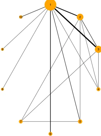
1 2 3 4 5 6 7 8 9 10

FIGURE 1 Network of trials of Diabetes application. Lines indicate that there is data available from one or more studies comparing the two treatments. Width of lines is proportional to the number of trials for that comparison. The size of the circle is proportional to the number of participants to that treatment

the mean HbA1c level at follow-up or the mean change in HbA1c level from baseline to follow-up. A total of 10 different treatment types were examined in these studies (1, placebo; 2, metformin; 3, rosiglitazone; 4, pioglita-zone; 5, acarbose; 6, miglitol; 7, sulfonylurea alone; 8, sitagliptin; 9, vildagliptin; 10, benfluorex). Figure 1 shows the plot of the network of this dataset. One study included 3 treatment arms, while the rest of the studies included 2 treatment arms. There are 16 different designs in the network. The available data are the sample mean, stan-dard deviation, and number of patients for each arm of each study. Firstly, we calculated each standard error of the sample mean. Since there is a continuous out-come available, a normal likelihood with identity link is used to fit the models for this application as described in Section 2.1. We have fitted the fixed effect model, the consistency model, and the Jackson model using both MCMC and INLA. To give some sense of how our nmaINLA package looks like in a routine data

analy-sis, below we show the corresponding R code to fit the

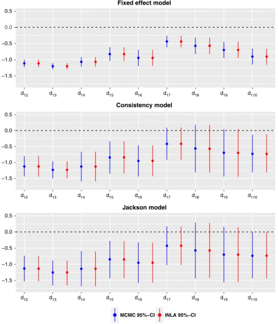
Figure 2 shows the posterior median and the 95% equi-tailed credible interval (CI) obtained by INLA and by MCMC for all basic parameter estimates of the 3 fitted models. The estimates of heterogeneity and inconsistency standard deviations are displayed in Table 1. Individual inconsistency random effects are displayed in Table 2.

Senn et al41_{have fitted fixed effect and consistency}

mod-els using frequentist methods to analyze the Diabetes data. Our results are in broad agreement with their results (see figures 5 and 7 in Senn et al41_).

The median and 95% equi-tailed CI of the heterogene-ity from Table 1 suggesting a substantial heterogeneheterogene-ity in the network. However, the estimates of the inconsistency are very close to zero, and also the individual inconsistency parameters from Table 2 are almost zero with high stan-dard deviations. Therefore, we can conclude that there is no evidence of substantial inconsistency in the network. The DIC values of the fixed effect model, the

consis-tency model, and the Jackson model are 36.86, −28.82,

and−28.27, respectively. The consistency model offers a

−1.5 −1.0 −0.5 0.0 0.5 −1.5 −1.0 −0.5 0.0 0.5 −1.5 −1.0 −0.5 0.0 0.5 d₁₂ d₁₃ d₁₄ d₁₅ d₁₆ d₁₇ d₁₈ d₁₉ d₁₁₀ Fixed effect model

Consistency model

Jackson model

MCMC 95%−CI INLA 95%−CI d

12 d13 d14 d15 d16 d17 d18 d19 d110

d₁₂ d₁₃ d₁₄ d₁₅ d₁₆ d₁₇ d₁₈ d₁₉ d₁₁₀

FIGURE 2 Median and 95% equi-tailed credible interval (CI) of the marginal posterior distributions of all relative treatment effects by MCMC and by INLA for the Diabetes data

TABLE 1 Estimates of heterogeneity and inconsistency standard deviation of consistency and Jackson model for the Diabetes application

Consistency Jackson MCMC INLA MCMC INLA Heterogeneity(𝝉) Posterior median 0.336 0.335 0.339 0.339 Lower b (95% CI) 0.217 0.218 0.216 0.216 Upper b (95% CI) 0.531 0.531 0.548 0.547 Inconsistency(𝜿) Posterior median 0.122 0.122 Lower b (95% CI) 0.006 0.007 Upper b (95% CI) 0.480 0.488

Abbreviations: INLA, integrated nested Laplace approximations; MCMC, Markov chain Monte Carlo.

TABLE 2 Estimated inconsistency parameters obtained from the fitted Jackson model for the Diabetes dataset

MCMC INLA

Design Parameter Mean Stdev Mean Stdev

1 𝜔1₁ ,2 −0.01 0.16 −0.01 0.15 2 𝜔2_1,5 −0.01 0.18 −0.01 0.17 𝜔2_1,2 −0.00 0.18 −0.00 0.18 3 𝜔3_1,3 0.04 0.16 0.04 0.16 4 𝜔4_1,4 −0.02 0.17 −0.02 0.17 5 𝜔5_2,4 0.03 0.18 0.03 0.17 6 𝜔6₃ ,4 −0.01 0.17 −0.00 0.17 7 𝜔7_2,3 0.00 0.17 −0.00 0.16 8 𝜔8_3,7 0.06 0.19 0.06 0.18 9 𝜔9_5,7 −0.00 0.18 −0.00 0.17 10 𝜔10_1,5 0.01 0.18 0.01 0.17 11 𝜔11_1,8 −0.00 0.20 −0.00 0.19 12 𝜔12₁ ,9 −0.00 0.20 −0.00 0.19 13 𝜔13_2,7 −0.06 0.19 −0.05 0.18 14 𝜔14_1,6 0.00 0.20 −0.00 0.19 15 𝜔15_2,3 0.02 0.17 0.02 0.17 16 𝜔16_1,10 0.00 0.20 −0.00 0.19

Abbreviations: INLA, integrated nested Laplace approximations; MCMC, Markov chain Monte Carlo.

large improvement in DIC compared to the fixed effect model, which confirms possible presence of the hetero-geneity. The DIC value of the Jackson model is very close to the DIC value of the consistency model. However, as displayed in Figure 2, including inconsistency random effects has considerable impact on the credible intervals (hence, the precisions) of the basic parameters. Therefore, although there is not strong evidence of any inconsistency in this network, it has quite considerable impact when it is included in the model.

1

2

3 4

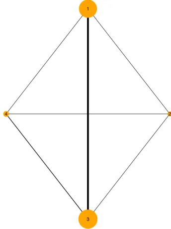
FIGURE 3 Network of trials of Smoking cessation

The MCMC and INLA methods gave very similar results. If we consider all 3 models, the largest absolute difference for the posterior median estimate based on MCMC and INLA among basic parameters was found in the Jackson

model ford18 (0.0059). Furthermore, the largest absolute

difference of the INLA and MCMC posterior mean esti-mates of individual inconsistency random effects in the Jackson model was 0.0032. For the Jackson model, the

MCMC run took 30 seconds while INLA only took

−1 0 1 2 3 d₁₂ d₁₃ d₁₄ d₁₂ d₁₃ d₁₄ Consistency model −1 0 1 2 3 Jackson model

MCMC 95%−CI INLA 95%−CI

FIGURE 4 Median and 95% equi-tailed credible interval (CI) of the marginal posterior distribution of all relative treatment effects by MCMC and by INLA for the Smoking cessation data

4.2

Smoking cessation: NMA

with dichotomous endpoints

The second application includes 24 trials investigating interventions to aid smoking cessation and has been

considered by Jackson et al12_{and Sauter and Held}25_among

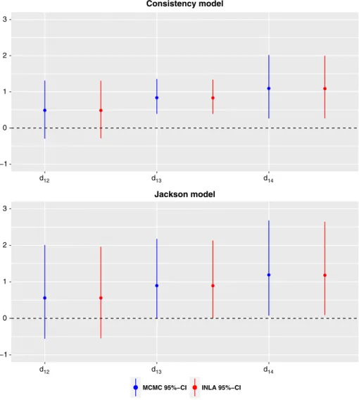
others. The number of individuals who successfully quits smoking after 6 to 12 months is reported for 4 different interventions (1 , no contact; 2 , self-help; 3 , individual counseling; and 4 , group counseling). The plot of the net-work is displayed in Figure 3. There are two 3-arm trials, one for treatments 1, 3, and 4 and one for treatments 2, 3, and 4. And there are 8 different designs in the network. Figure 4 shows the posterior median and the 95% equi-tailed CI obtained by INLA and by MCMC for basic parameter estimates of the consistency and the Jackson model. Furthermore, the marginal posterior densities from the Jackson model are displayed in Figure 5 as histograms of the MCMC samples and as solid lines of the INLA

results. Finally, Table 3 demonstrates the estimates of inconsistency random effects obtained by MCMC and

INLA. Jackson et al12_{presented the fitted consistency and}

Jackson model using MCMC for the Smoking dataset. We obtained very similar results with the results displayed in table 3 of Jackson et al.12

The posterior median for the heterogeneity standard deviation is 0.82 with 95% CI [0.55, 1.3] suggesting that there may be notable heterogeneity in the network. The posterior median for the inconsistency standard deviation is 0.4 with 95% CI [0.02, 1.87], suggesting moderate but highly uncertain inconsistency. Moreover, when we exam-ine the inconsistency random effects in Table 3, it is hard to claim that there is strong evidence for the inconsistency in this network, since standard deviations are very wide. The DIC values of the consistency model, and the Jackson model are 326.56 and 326.62, respectively. Since the DIC values are almost indistinguishable, we may conclude that no strong inconsistency in the network. On the other hand,

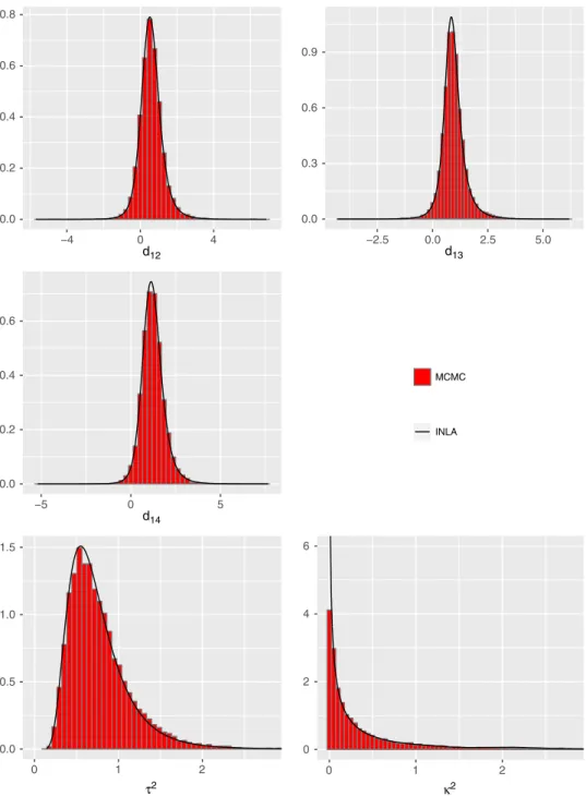
0.0 0.2 0.4 0.6 0.8 −4 0 4 d₁₂ 0.0 0.3 0.6 0.9 −2.5 0.0 2.5 5.0 d₁₃ 0.0 0.2 0.4 0.6 −5 0 5 d₁₄ MCMC INLA 0.0 0.5 1.0 1.5 0 1 2 τ2 0 2 4 6 0 1 2 κ2

FIGURE 5 Marginal posterior density estimates of all basic parameters, the heterogeneity and inconsistency variances by MCMC (histogram) and by INLA (straight line) obtained from the fitted Jackson model for the Smoking cessation dataset

as in the Diabetes application, including inconsistency parameters to the consistency model influences the precision of the basic parameters, which can be seen from

Figure 4. This observation was also made by Jackson et al.12

We can conclude that both inference techniques, MCMC and INLA, give similar results in our analysis. Based on MCMC and INLA of the fitted Jackson model, the largest absolute difference for the posterior median esti-mate of the basic parameters was 0.0035 and for the pos-terior mean estimate of the inconsistency parameters was

0.017(𝜔5₁₄). For the Jackson model, the MCMC run took

34.2 seconds while the computing time was 6.5 seconds with INLA.

4.3

Stroke prevention:

network meta-regression

with dichotomous endpoints

Data have been collected and analyzed by Batson et al,39

and the raw data are given in the supporting information of their paper. Stroke data include 19 studies that compare 15 different treatments to prevent stroke in patients

TABLE 3 Estimated inconsistency parameters obtained from the fitted Jackson model for the Smoking dataset

MCMC INLA

Design Parameter Mean Stdev Mean Stdev

1 𝜔1₁ ,3 0.03 0.54 0.02 0.53 𝜔1_1,4 −0.26 0.63 −0.28 0.64 2 𝜔2_2,3 −0.06 0.54 −0.07 0.55 𝜔2_2,4 −0.09 0.54 −0.10 0.55 3 𝜔3₁ ,3 −0.08 0.50 −0.10 0.50 4 𝜔4_1,2 −0.12 0.56 −0.13 0.55 5 𝜔5_1,4 0.39 0.77 0.39 0.76 6 𝜔6_2,3 −0.10 0.54 −0.11 0.55 7 𝜔7₂ ,4 0.10 0.55 0.09 0.55 8 𝜔8_3,4 −0.04 0.51 −0.03 0.50

Abbreviations: INLA, integrated nested Laplace approximations; MCMC, Markov chain Monte Carlo.

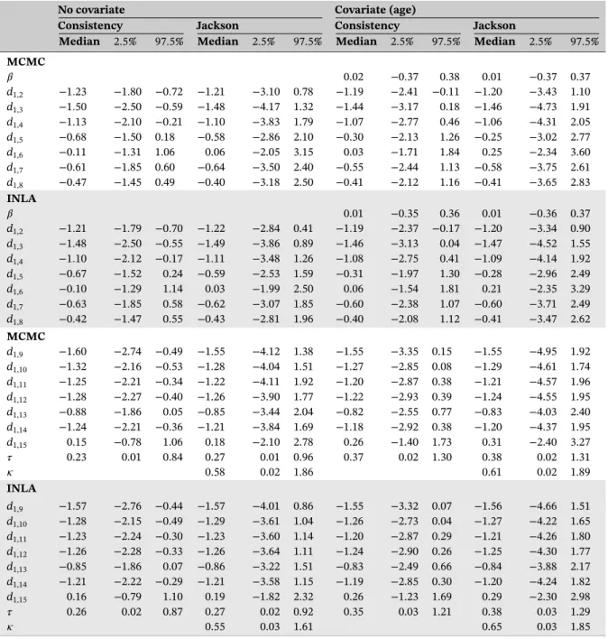
with atrial fibrillation (AF). Treatments include fixed low-dose warfarin with or without aspirin, aspirin monotherapy, aspirin plus clopidogrel, indobufen, idra-parinux, triflusal, and ximelagatran. The corresponding network plot is given in Figure 6. The primary outcome was the number of patients who had stroke events, a dichotomous end point. The study-level covariate of mean age is available. We fit a network meta-regression model as described in Section 2.4 using both MCMC and INLA. Placebo was chosen to be the reference treatment. Note that since one study does not have the mean age informa-tion, the corresponding network meta-regression model reduced in size by one (hence, 18 studies). In the net-work meta-regression models, the interaction coefficient

(𝛽) is common for all treatment versus placebo. Table 4

displays the results of the fitted consistency and Jackson model with no covariate and with covariate information (mean age) using MCMC and INLA. Moreover, individual inconsistency random effects of the Jackson model with-out the covariate information are displayed in Table 5. Our results are in broad agreement with Figure 2 and Table 1 of Batson et al.39

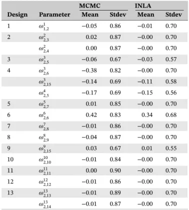
From the Jackson model using INLA, the poste-rior median of the heterogeneity standard deviation is 0.27 with 95% CI [0.02, 0.92] suggesting moderate heterogeneity in the network. The posterior median of the inconsistency standard deviation is 0.55 with 95% CI [0.03, 1.61], suggesting there may be notable inconsis-tency with high uncertainty in the network. The DIC values of the consistency model and the Jackson model without covariates are 283.05 and 283.72, respectively, which shows that adding inconsistency parameters does not result any improvement in DIC. From the results of

individual inconsistency random effects, only𝜔3₂₆and𝜔6₂₆

1 2 3 4 5 6 7 8 9 10 11 12 13 14 15

FIGURE 6 Network of trials of Stroke data

are relatively large but with very wide standard devia-tions. On the other hand, the addition of a covariate to the consistency model and the Jackson model, actually, increase the estimates of both heterogeneity and

incon-sistency standard deviations (𝜏 and 𝜅). The DIC values

of the consistency model and the Jackson model with covariates are 271.31 and 272.05, respectively. To compare the models with covariate and without covariate infor-mation, we calculate the DIC values of the consistency

TABLE 4 Quantiles of the marginal posterior distributions of basic parameters, heterogeneity, and inconsistency standard deviations by MCMC (top) and INLA (bottom) for Stroke application

No covariate Covariate (age)

Consistency Jackson Consistency Jackson

Median 2.5% 97.5% Median 2.5% 97.5% Median 2.5% 97.5% Median 2.5% 97.5% MCMC 𝛽 0.02 −0.37 0.38 0.01 −0.37 0.37 d1,2 −1.23 −1.80 −0.72 −1.21 −3.10 0.78 −1.19 −2.41 −0.11 −1.20 −3.43 1.10 d1,3 −1.50 −2.50 −0.59 −1.48 −4.17 1.32 −1.44 −3.17 0.18 −1.46 −4.73 1.91 d1,4 −1.13 −2.10 −0.21 −1.10 −3.83 1.79 −1.07 −2.77 0.46 −1.06 −4.31 2.05 d1,5 −0.68 −1.50 0.18 −0.58 −2.86 2.10 −0.30 −2.13 1.26 −0.25 −3.02 2.77 d1,6 −0.11 −1.31 1.06 0.06 −2.05 3.15 0.03 −1.71 1.84 0.25 −2.34 3.60 d1,7 −0.61 −1.85 0.60 −0.64 −3.50 2.40 −0.55 −2.44 1.13 −0.58 −3.75 2.61 d1,8 −0.47 −1.45 0.49 −0.40 −3.18 2.50 −0.41 −2.12 1.16 −0.41 −3.65 2.83 INLA 𝛽 0.01 −0.35 0.36 0.01 −0.36 0.37 d1,2 −1.21 −1.79 −0.70 −1.22 −2.84 0.41 −1.19 −2.37 −0.17 −1.20 −3.34 0.90 d1,3 −1.48 −2.50 −0.55 −1.49 −3.86 0.89 −1.46 −3.13 0.04 −1.47 −4.52 1.55 d1,4 −1.10 −2.12 −0.17 −1.11 −3.48 1.26 −1.08 −2.75 0.41 −1.09 −4.14 1.92 d1,5 −0.67 −1.52 0.24 −0.59 −2.53 1.59 −0.31 −1.97 1.30 −0.28 −2.96 2.49 d1,6 −0.10 −1.29 1.14 0.03 −1.99 2.50 0.06 −1.54 1.81 0.21 −2.35 3.29 d1,7 −0.63 −1.85 0.58 −0.62 −3.07 1.85 −0.60 −2.38 1.07 −0.60 −3.71 2.49 d1,8 −0.42 −1.47 0.55 −0.43 −2.81 1.96 −0.40 −2.08 1.12 −0.41 −3.47 2.62 MCMC d1,9 −1.60 −2.74 −0.49 −1.55 −4.12 1.38 −1.55 −3.35 0.15 −1.55 −4.95 1.92 d1,10 −1.32 −2.16 −0.53 −1.28 −4.04 1.51 −1.27 −2.85 0.08 −1.29 −4.61 1.74 d1,11 −1.25 −2.21 −0.34 −1.22 −4.11 1.92 −1.20 −2.87 0.38 −1.21 −4.57 1.96 d1,12 −1.28 −2.27 −0.40 −1.26 −3.90 1.77 −1.22 −2.93 0.39 −1.24 −4.55 1.95 d1,13 −0.88 −1.86 0.05 −0.85 −3.44 2.04 −0.82 −2.55 0.77 −0.83 −4.03 2.40 d1,14 −1.24 −2.21 −0.36 −1.21 −3.84 1.69 −1.18 −2.92 0.38 −1.20 −4.37 1.95 d1,15 0.15 −0.78 1.06 0.18 −2.10 2.78 0.26 −1.40 1.73 0.31 −2.40 3.27 𝜏 0.23 0.01 0.84 0.27 0.01 0.96 0.37 0.02 1.30 0.38 0.02 1.31 𝜅 0.58 0.02 1.86 0.61 0.02 1.89 INLA d1,9 −1.57 −2.76 −0.44 −1.57 −4.01 0.86 −1.55 −3.32 0.07 −1.56 −4.66 1.51 d1,10 −1.28 −2.15 −0.49 −1.29 −3.61 1.04 −1.26 −2.73 0.04 −1.27 −4.22 1.65 d1,11 −1.23 −2.24 −0.30 −1.23 −3.60 1.14 −1.20 −2.87 0.29 −1.21 −4.26 1.80 d1,12 −1.26 −2.28 −0.33 −1.26 −3.64 1.11 −1.24 −2.90 0.26 −1.25 −4.30 1.77 d1,13 −0.85 −1.86 0.07 −0.86 −3.22 1.51 −0.83 −2.49 0.66 −0.84 −3.88 2.17 d1,14 −1.21 −2.22 −0.29 −1.21 −3.58 1.15 −1.19 −2.85 0.30 −1.20 −4.24 1.82 d1,15 0.16 −0.79 1.10 0.19 −1.82 2.32 0.26 −1.23 1.69 0.29 −2.30 2.98 𝜏 0.26 0.02 0.87 0.27 0.02 0.92 0.35 0.03 1.21 0.38 0.03 1.29 𝜅 0.55 0.03 1.61 0.65 0.03 1.85

Note: The first line shows the estimate for the interaction coefficient(𝛽). INLA, integrated nested Laplace approximations; MCMC, Markov chain Monte Carlo.

model and the Jackson model without covariate when we drop the study, which does not have mean-age informa-tion, and the results are 269.78 and 270.58, respectively. This suggests that adding covariates does not offer any notable improvement in the DIC values. Furthermore, from the results of the Jackson model with covariate,

the posterior median estimate of𝛽 is 0.01 with 95% CI

[−0.36,0.37]. Therefore, we can conclude that the inclu-sion of mean-age covariate to the model fails to explain the source of heterogeneity and/or the inconsistency in the network.

Both methods MCMC and INLA gave similar results. Approximately, the MCMC run took 27.1 seconds, while INLA took only 5.4 seconds for the Jackson model with covariate.

5

DISCUSSION

We have presented an approximate Bayesian inference technique, INLA, to fit various contrast-based NMA models with arm-based likelihood including the Jack-son model as well as their network meta-regression

TABLE 5 Estimated inconsistency parameters obtained from the fitted Jackson model for the Stroke dataset

MCMC INLA

Design Parameter Mean Stdev Mean Stdev

1 𝜔1_1,2 −0.05 0.86 −0.01 0.70 2 𝜔2₂ ,3 0.02 0.87 −0.00 0.70 𝜔2_2,4 0.00 0.87 −0.00 0.70 3 𝜔3_2,5 −0.06 0.67 −0.03 0.57 4 𝜔3_2,6 −0.38 0.82 −0.00 0.70 𝜔3₂ ,15 −0.14 0.69 −0.11 0.58 𝜔4_2,5 −0.17 0.69 −0.15 0.56 5 𝜔5_2,7 0.01 0.85 −0.00 0.70 6 𝜔6_2,6 0.42 0.83 0.34 0.68 7 𝜔7₂ ,8 −0.01 0.86 −0.00 0.70 8 𝜔8_2,9 −0.04 0.87 −0.00 0.70 9 𝜔9_2,15 0.03 0.67 0.01 0.55 10 𝜔10_2,10 −0.01 0.84 −0.00 0.70 11 𝜔11₂ ,11 0.00 0.90 −0.00 0.70 12 𝜔12_2,12 −0.01 0.86 −0.00 0.70 13 𝜔13_2,13 −0.01 0.89 −0.00 0.70 𝜔13_2,14 −0.01 0.87 −0.00 0.70

Abbreviations: INLA, integrated nested Laplace approximations; MCMC, Markov chain Monte Carlo.

extensions. Furthermore, to make it more accessible

for researchers, we provide an R package, nmaINLA,

which automates INLA implementation of NMA mod-els. There are good reasons to prefer INLA to MCMC. Firstly, INLA has better time performance. Secondly, there is no need to check any MCMC convergence diagnos-tics. Actually, this is very crucial for a large network, since the number of parameters to check diagnostics is increasing dramatically.

There is an ongoing debate about merits of the contrast-based (CB) models and the arm-based (AB) models. Relative treatment effect are assumed to be exchangeable across trials in the CB approach, whereas AB approach assumes that absolute treatment effects are

exchangeable.8_{The supporters of CB approach claim that}

“arm-based pooling effectively breaks randomization, and in fact runs against the entire way in which

random-ized controlled trials are designed, analysed, and used .”8

AB modelers respond that “although AB models require different assumptions than CB models, it is not obvious that they are less reasonable, and the payoffs they can pro-vide (significantly increased modeling flexibility, as well as greater ease of interpretation, prior specification, and

model fitting) can be substantial.”9 _{For our concern, AB}

models are also in the family of LGMs. Therefore, it is certainly possible to use INLA to fit AB models, although

our package nmaINLA does not support AB models,

yet. Alternative to the Jackson model, the node-splitting

method10 _{is another method to detect network}

incon-sistencies. Although we have not discussed this method

and not implemented it in nmaINLA; INLA of course

could be used. The explanations and the necessaryR-code

are presented in Sauter and Held.25

One may find it restrictive to assume that heterogene-ity and inconsistency random effects are normally dis-tributed, hence explore different distributions for this

assumption, for instance, t distribution.42 _{Although this}

modeling approach is not in the scope of latent Gaussian models, INLA still can be used as an inference tool for such models.43

Unfortunately, there is no analytical expression for the approximation error obtained by INLA. A simple way to investigate its accuracy is comparison with long MCMC runs. The accuracy of INLA for fitting GLMMs has been

investigated in rich simulation studies by Fong et al31

and Grilli et al.44_{They reported INLA works very well in}

most cases, but in some extreme cases, of binary GLMMs with few or zero events per variable, INLA exhibits some inaccuracy. Moreover, for the special situation when a covariate (almost) perfectly predicts the response (quasi-complete separation) in binary response GLMMs, Sauter

INLA is substantial. Ferkingstad and Rue46 _{introduced a} copula-based correction, which significantly increase the accuracy of INLA for such extreme cases of GLMMs,

and it is already implemented in R-INLA. As a matter

of fact, in the case of such “sparse data” situations47 _of

binary GLMM, it is known that both maximum likelihood methods and Bayesian inference with vague priors may

result serious bias away from the null.48 _{Hence, different}

penalization techniques of maximum likelihood estimates (MLE) or using weakly informative priors for Bayesian

inference have been advocated to avoid such biases.49_Such

problems may occur in the NMA context as well, espe-cially when the model is a binary GLMM. Therefore, network meta-analyzer should be cautious not to obtain biased results regardless of his/her inference tool (MLE, MCMC, or INLA).

Using vague priors for hyperparameters of NMA models may make it extremely hard to identify these parameters. This can be overcome by using more informative priors. Using predictive distributions as priors for

hyperparame-ters to fit the Jackson model is proposed by Law et al.17

On the other hand, Simpson et al50_{has been introduced a}

principled and broad framework to construct prior distri-bution for a large class of hierarchical models. The priors

that they develop, PC priors, are implemented inR-INLA;

hence, they can be used in a NMA context, especially for constructing priors for hyperparameters. Moreover, checking sensitivity of heterogeneity and inconsistency parameters to the chosen prior distributions may be par-ticularly useful for NMA models. Although we did not discuss any sensitivity analysis, it can be easily conducted

due to the computational speed of INLA.51 _{We note that}

the standard ranking of treatments as discussed in Lu

and Ades2 _{is not possible using INLA. Although point}

estimates of ranking of treatments are provided, it is not possible to estimate the associated errors using INLA. This is because INLA is computing marginal posteriors but not joint posteriors. On the other hand, the standard ranking may be misleading since it does not take other evidences into account.52

ACKNOWLEDGMENTS

We thank Rafael Sauter who wrote the first version of the

RpackagenmaINLA, Sarah Batson who kindly answered

our questions regarding the Stroke application discussed in Section 4.3, and Christian Röver for carefully proofreading this manuscript. We also like to thank 2 anonymous reviewers who recommended several changes that lead to substantial improvements and an improved presenta-tion of this paper. This research has received funding from the EU's 7th Framework Programme for research, tech-nological development and demonstration under grant

agreement number FP HEALTH 2013-602144 with

project title (acronym) “Innovative Methodology for Small Populations Research” (InSPiRe).

ORCID

Burak Kürsad Günhan http://orcid.org/ 0000-0002-7454-8680

REFERENCES

1. Lumley T. Network meta-analysis for indirect treatment com-parisons.Stat Med. 2002;21:2313-2324.

2. Lu G, Ades AE. Assessing evidence inconsistency in mixed treatment comparisons.J Am Stat Assoc. 2006;101:447-459. 3. Higgins JPT, Thompson SG, Spiegelhalter DJ. A re-evaluation

of random-effects meta-analysis.J R Stat Soc Ser A Stat Soc. 2009;172:137-159.

4. Salanti G. Indirect and mixed-treatment comparison, network, or multiple-treatments meta-analysis: many names, many ben-efits, many concerns for the next generation evidence synthesis tool.Res Syn Meth. 2012;3:80-97.

5. Higgins JPT, Welton NJ. Network meta-analysis: a norm for comparative effectiveness?.Lancet. 2015;386:628-630.

6. Hawkins N, Scott DA, Woods B. 'Arm-based' parameterization for network meta-analysis.Res Syn Meth. 2016;7:306-313. 7. Piepho HP. Network-meta analysis made easy: detection of

inconsistency using factorial analysis-of-variance models.BMC Med Res Methodol. 2014;14:1-9.

8. Dias S, Ades AE. Absolute or relative effects? Arm-based synthe-sis of trial data.Res Syn Meth. 2016;7:23-28.

9. Hong H, Chu H, Zhang J, Carlin BP. Rejoinder to the discussion of “a Bayesian missing data framework for generalized multi-ple outcome mixed treatment comparisons” by S. Dias and A.E. Ades.Res Syn Meth. 2016;7:29-33.

10. Dias S, Welton NJ, Caldwell DM, Ades AE. Checking consis-tency in mixed treatment comparison meta-analysis.Stat Med. 2010;29:932-944.

11. Higgins JPT, Jackson D, Barrett JK, Lu G, Ades AE, White IR. Consistency and inconsistency in network meta-analysis: concepts and models for multi-arm studies. Res Syn Meth. 2012;3:98-110.

12. Jackson D, Barrett JK, Rice S, White IR, Higgins JPT. A design-by-treatment interaction model for network meta-analysis with random inconsistency effects. Stat Med. 2014;33:3639-3654.

13. Dias S, Sutton AJ, Welton NJ, Ades AE. Evidence synthesis for decision making 3: Heterogeneity-subgroups, meta-regression, bias, and bias-adjustment.MDM Policy Pract. 2013;33: 618-640.

14. Jackson D, Law M, Barrett JK, et al. Extending Dersimonian and Laird's methodology to perform network meta-analyses with random inconsistency effects.Stat Med. 2016;35:819-839. 15. Jackson D, Bujkiewicz S, Law M, Riley RD, White IR.

A matrix-based method of moments for fitting multivariate network meta-analysis models with multiple outcomes and ran-dom inconsistency effects.Biometrics. 2017. https://doi.org/10. 1111/biom.12762

16. DerSimonian R, Laird N. Meta-analysis in clinical trials.Control Clin Trials. 1986;7:177-188.

17. Law M, Jackson D, Turner R, Rhodes K, Viechtbauer W. Two new methods to fit models for network meta-analysis

with random inconsistency effects. BMC Med Res Methodol. 2016;16:87.

18. Jackson D, Veroniki A, Law M, Tricco AC, Baker R. Paule-mandel estimators for network meta-analysis with random inconsistency effects.Res Syn Meth. 2017;8:416-434. 19. Lunn DJ, Thomas A, Best N, Spiegelhalter D. WinBUGS—a

Bayesian modelling framework: concepts, structure, and exten-sibility.Stat Comput. 2000;10:325-337.

20. Lunn D, Spiegelhalter D, Thomas A, Best N. The BUGS project: evolution, critique and future directions. Stat Med. 2009;28:3049-3067.

21. Plummer M. JAGS: a program for analysis of Bayesian graphical models using Gibbs sampling. In: Proceedings of the 3rd Inter-national Workshop on Distributed Statistical Computing; 2003; Vienna, Austria. 1-11.

22. Stan Development Team. Stan modeling language user's guide and reference manual, version 2.12.0; 2016.

23. Rue H, Martino S, Chopin N. Approximate Bayesian infer-ence for latent Gaussian models by using integrated nested Laplace approximations. J R Stat Soc Series B Stat Methodol. 2009;71:319-392.

24. Paul M, Riebler A, Bachmann LM, Rue H, Held L. Bayesian bivariate meta-analysis of diagnostic test studies using integrated nested Laplace approximations. Stat Med. 2010;29:1325-1339.

25. Sauter R, Held L. Network meta-analysis with integrated nested Laplace approximations.Biom J. 2015;57:1038-1050.

26. Dias S, Welton NJ, Sutton AJ, Ades AE. NICE DSU Technical Support Document 2: A generalised linear modelling frame-work for pairwise and netframe-work meta-analysis of randomised controlled trials. last updated September 2016; 2011.

27. Higgins JPT, Whitehead A. Borrowing strength from external trials in a meta-analysis.Stat Med. 1996;15:2733-2749.

28. Jackson D, Boddington P, White IR. The design-by-treatment interaction model: a unifying framework for modelling loop inconsistency in network meta-analysis. Res Syn Meth. 2016;7:329-332.

29. Thompson SG, Higgins JPT. How should meta-regression analyses be undertaken and interpreted?. Stat Med. 2002;21:1559-1573.

30. Cooper NJ, Sutton AJ, Morris D, Ades AE, Welton NJ. Address-ing between-study heterogeneity and inconsistency in mixed treatment comparisons: application to stroke prevention treat-ments in individuals with non-rheumatic atrial fibrillation.Stat Med. 2009;28:1861-1881.

31. Fong Y, Rue H, Wakefield J. Bayesian inference for generalized linear mixed models.Biostatistics. 2010;11:397-412.

32. Rue H, Riebler A, Sørbye SH, Illian JB, Simpson DP, Lindgren FK. Bayesian computing with INLA: a review.Annu Rev Stat Appl. 2017:395-421.

33. Tierney L, Kadane JB. Accurate approximations for pos-terior moments and marginal densities. J Am Stat Assoc. 1986;81:82-86.

34. Blangiardo M, Cameletti M. Bayesian computing.Spatial and spatio-temporal Bayesian models with R-INLA. New York: John Wiley & Sons, Ltd; 2015:75-126.

35. Rue H, Riebler A, Sørbye SH, Illian JB, Simpson DP, Lindgren FK. Bayesian computing with inla: new features.Comput Stat Data Anal. 2013;67:68-83.

36. Spiegelhalter DJ, Best NG, Carlin BP, Van Der Linde A. Bayesian measures of model complexity and fit.J R Stat Soc Series B Stat Methodol. 2002;64:583-639.

37. Watanabe S. Asymptotic equivalence of bayes cross valida-tion and widely applicable informavalida-tion criterion in singular

learning theory. J Mach Learn Res. December 2010;11: 3571-3594.

38. Su Y, Yajima M. R2jags: Using R to run 'JAGS'. R package version 0.5-7; 2015.

39. Batson S, Sutton A, Abrams K. Exploratory network meta regres-sion analysis of stroke prevention in atrial fibrillation fails to identify any interactions with treatment effect.PLoS One. 2016;11(8):1-12. e0161864.

40. Gelman A, Rubin DB. Inference from iterative simulation using multiple sequences.Stat Sci. 1992;7:457-472.

41. Senn S, Gavini F, Magrez D, Scheen A. Issues in performing a network meta-analysis.Stat Methods Med Res. 2013;22:169-189. 42. Lee KJ, Thompson SG. Flexible parametric models for

random-effects distributions.Stat Med. 2008;27:418-434. 43. Martins TG, Rue H. Extending integrated nested Laplace

approximation to a class of near-Gaussian latent models.Scand Stat Theory Appl. 2014;41:893-912.

44. Grilli L, Metelli S, Rampichini C. Bayesian estimation with integrated nested Laplace approximation for binary logit mixed models.J Stat Comput Simul. 2015;85:2718-2726.

45. Sauter R, Held L. Quasi-complete separation in random effects of binary response mixed models. J Stat Comput Simul. 2016;86:2781-2796.

46. Ferkingstad E, Rue H. Improving the inla approach for approx-imate bayesian inference for latent gaussian models.Electron J Stat. 2015;9:2706-2731.

47. Greenland S, Mansournia MA, Altman DG. Sparse data bias: a problem hiding in plain sight.BMJ. 2016;352:1-6.

48. Gelman A, Jakulin A, Pittau MG, Su Y. A weakly informa-tive default prior distribution for logistic and other regression models.Ann Appl Stat. 200812;2:1360-1383.

49. Greenland S, Mansournia MA. Penalization, bias reduction, and default priors in logistic and related categorical and survival regressions.Stat Med. 2015;34:3133-3143.

50. Simpson D, Rue H, Riebler A, Martins TG, Sørbye SH. Penalising model component complexity: a principled, practical approach to constructing priors.Stat Sci. 2017;32:1-28.

51. Roos M, Martins TG, Held L, Rue H. Sensitivity anal-ysis for Bayesian hierarchical models. Bayesian Anal. 201506;10:321-349.

52. Puhan MA, Schünemann HJ, Murad MH, et al. A grade work-ing group approach for ratwork-ing the quality of treatment effect estimates from network meta-analysis.BMJ. 2014;349:1-10.

SUPPORTING INFORMATION

Additional Supporting Information may be found online in the supporting information tab for this article.

How to cite this article: Günhan BK, Friede T, Held L. A design-by-treatment interaction model for network meta-analysis and meta-regression with

integrated nested Laplace approximations. Res Syn