POPULARITY SHOCKS AND POLITICAL SELECTION
Francisco Cavalcanti, Gianmarco Daniele, Sergio GallettaIEB Working Paper
2018/04
IEB Working Paper 2018/04
POPULARITY SHOCKS AND POLITICAL SELECTION
Francisco Cavalcanti, Gianmarco Daniele, Sergio Galletta
The Barcelona Institute of Economics (IEB) is a research centre at the University of Barcelona (UB) which specializes in the field of applied economics. The IEB is a foundation funded bythe following institutions: Applus, Abertis, Ajuntament de Barcelona, Diputació de Barcelona, Gas Natural, La Caixa and Universitat de Barcelona.
The IEB research program in Fiscal Federalism aims at promoting research in the public finance issues that arise in decentralized countries. Special emphasis is put on applied research and on work that tries to shed light on policy-design issues. Research that is particularly policy-relevant from a Spanish perspective is given special consideration. Disseminating research findings to a broader audience is also an aim of the program. The program enjoys the support from the IEB-Foundation and the IEB-UB Chair in Fiscal Federalism funded by Fundación ICO, Instituto de Estudios Fiscales and Institut d’Estudis Autonòmics.
Postal Address:
Institut d’Economia de Barcelona Facultat d’Economia i Empresa Universitat de Barcelona C/ John M. Keynes, 1-11 (08034) Barcelona, Spain Tel.: + 34 93 403 46 46 [email protected] http://www.ieb.ub.edu
The IEB working papers represent ongoing research that is circulated to encourage discussion and has not undergone a peer review process. Any opinions expressed here are those of the author(s) and not those of IEB.
IEB Working Paper 2018/04
POPULARITY SHOCKS AND POLITICAL SELECTION *
Francisco Cavalcanti, Gianmarco Daniele, Sergio Galletta
ABSTRACT: We observe that popularity shocks are crucial for electoral accountability beyond their effects on voters’ behaviors. By focusing on Brazilian politics, we show that the disclosure of audit reports on the (mis)use of federal funds by local administrators affects the type of candidates who stand for election. When the audit finds low levels of corruption, the parties supporting the incumbent select less-educated candidates. On the contrary, parties pick more-educated candidates when the audit reveals a high level of corruption. These effects are stronger in municipalities that have easier access to local media.
JEL Codes: D70, D72, D73
Keywords: Political selection, corruption, competence, local election, political parties
Francisco Cavalcanti Universitat de Barcelona &
Institut d’Economia de Barcelona (IEB) E-mail: [email protected]
Gianmarco Daniele
Bocconi University (Baffi Carefin) & Institut d’Economia de Barcelona (IEB) E-mail: [email protected] Sergio Galletta
Universitat de Barcelona,
Institut d’Economia de Barcelona (IEB), Institute of Economics (IdEP) &
University of Lugano (USI) E-mail: [email protected]
*
We are grateful to Toke Aidt, Massimo Bordignon, Fernanda Brollo, Pamela Campa, Claudio Ferraz, Diogo Gerhard, Benny Geys, Miriam Golden, Roland Hodler, Mario Jametti, Stephan Litschig, Eva Mörk, Hannes Mueller, Torsten Persson, Dina Pomeranz, Didac Queralt, Albert Solé-Ollé and Ragnar Torvik for valuable comments and suggestions. We have also benefited from comments by participants at the Sinergia Workshop (Basel), SIEP (Lecce), SSES (Lausanne) and seminars at the Universities of Barcelona, Warwick, Lugano and ETHZ - KOF in Zürich. Sergio Galletta gratefully acknowledges financial support from the Swiss National Science Foundation (grants Early Postdoc.Mobility – 15860 and Advanced Postdoc.Mobility – 167635). Gianmarco Daniele gratefully acknowledges financial support from the Recercaixa project: “Limits to political corruption: Media, party systems, civil society and citizens” (2016ACUP 00177).
1. Introduction
Electoral accountability is a crucial mechanism that helps guarantee the sustainability of modern democracies. It allows sufficiently informed voters to assess the government’s performance and hold politicians accountable for their actions (Barro, 1973; Mayhew, 1974). An extensive empirical literature shows that voters reduce their support of parties and officials involved in political scandals and reward politicians who are perceived to perform better (Ashworth, 2012; Ferraz and Finan, 2008; Snyder and Hirano, 2012; Chong et al., 2015; Costas-Pérez et al., 2012; Bagues and Esteve-Volart, 2016).1
In this paper, we follow up on these findings and account for the possibility that polit-ical parties might anticipate voters’ punishment, or reward, and change the composition of the pool of candidates selected to run for office accordingly. Specifically, we show that the release of information about government corruption affects the quality of candidates of the incumbent coalition. Intuitively, one might expect that if a political party (or coalition of parties) supports a government that faces a negative popularity shock, it might react by selecting more appealing and competent candidates to compensate for the expected poor results in the following election. Symmetrical intuitions could hold if there is a positive popularity shock: one might expect the party to behave strategically by reducing the share of costly, high-ability candidates given that the election will be less competitive.2 These ideas are closely related to a recent strand of literature showing that political parties are strategic players that take into account specific features of the electoral competition when making decisions (Galasso and Nannicini, 2011; Mattozzi and Merlo, 2015).
We address this issue in the Brazilian context by looking at the effect of popular-ity shocks resulting from the disclosure of reports about potential misconduct in local governments on the ability of candidates for city councilor in the 2004 and 2008 local elections. Hence, we relate the education level of candidates from the coalition support-1Interestingly, this effect might not arise when voters already believe politicians to be malfeasant
Arias et al. (2017) or when the media market structure does not provide incentives to supply politically-relevant information to their audiences Larreguy et al. (2017).
2We follow recent studies by considering education level as a proxy for politicians’ ability. See, for
example, Ferraz and Finan (2009), Galasso and Nannicini (2011), Gagliarducci and Nannicini (2013), Besley et al. (2011) or Daniele and Geys (2015). In the next section, we discuss the reasons and the implications of the fact that high ability candidates are costly for political parties.
ing (or opposing) the incumbent government with the release of information about its (dis)honesty. This information was made available to voters through an anti-corruption program introduced in 2003 by the Brazilian central government that monitors how mu-nicipalities spend federal funds. The primary task is performed by auditors who examine municipalities’ accounts to verify the correct use of federal transfers.
Municipalities are randomly selected into the anti-corruption program, and the tim-ing of the release of the report is also random. These characteristics are crucial for our identification strategy, as they help to assess the multi-faceted endogeneity issue of link-ing government conduct and the general quality of local politicians. Another important aspect for our purposes is that the process of selecting candidates for the city council has a similar schedule in all Brazilian municipalities. This makes it possible to define when, during the term, the selection process is taking place. Further, although city councilors are elected using an open-list proportional system, parties play a central role in selecting candidates. In practice, a citizen is eligible to stand for election if he has been affiliated with the supporting party for at least 12 months before election day. Formally, the candidate list is decided during party conventions that, by law, are held in June of each election year. This list must be submitted at least 3 months before election day.
We exploit the randomness of the timing of corruption disclosures and, conditioning on the level of corruption, compare the ability of the pool of candidates in municipalities where the audits were released during the candidate selection period (i.e., from 12 to 3 months before the election) with that of municipalities in which the audits were released either before or after the selection period. While our identification strategy closely follows the one used in Ferraz and Finan (2008), we define treatment slightly differently to suit our distinct research question.
Our findings, which are based on 1,321 municipalities that were audited in the period 2003–2010, show that when reports are disclosed during the political selection period, they lead to a significant change in the average ability of the candidates running for the city council who belong to the party (or coalition) of the incumbent mayor.3 This effect crucially depends on the level of corruption reported. Indeed, the spread of in-formation about government conduct can provide either a positive or negative shock to the expected electoral results, depending on citizens’ prior beliefs about the quality of the government (Besley, 2007). On the one hand, we find that there is a decrease in
the candidates’ average education of nearly 4.5 months of schooling when low levels of corruption are reported (i.e., lower than the median). On the other hand, we find an increase of nearly 4 months of schooling when substantial corruption is reported (i.e., higher than the median). In other words, there is a difference of 8.5 months of schooling depending on the results of the audit, which corresponds to about 30–35% of one stan-dard deviation. These symmetric results are not surprising in a context where trust in politics is very low, and releasing information about the absence of corruption could be more unexpected than the opposite.4 The effect is of a similar magnitude when consider-ing the sample of freshmen candidates or when we look at the median level of education. Interestingly, the effect is larger when we constrain our analysis to municipalities that have easier access to information due to the existence of local radio stations. Indeed, our findings are confirmed when using a different proxy for candidates’ ability, i.e. in-dividuals’ main occupation. However, we do not find any change in other observable characteristics such as age and gender. Moreover, the undesirable selection of low ability candidates in municipalities that experience a positive popularity shock fades away the closer the release of the audit report is to the election. Finally, we find that changing the composition of the candidate pool does not have a significant effect on electoral out-comes. In fact, voters still punish corrupt parties, in particular where local radio stations are available, and the elected candidates do not appear to have different characteristics compared to those elected in municipalities where the report was released outside the selection period.
To our knowledge, we are the first to estimate the effect of popularity shocks about the incumbent government on the quality of political candidates. Our findings are closely related to the recent literature that emphasizes that the characteristics of the electoral race affect candidate selection. This could be caused by a change in either individuals’ incentives to enter politics or parties’ incentives to select particular types of candidates (Caselli and Morelli, 2004; Galasso and Nannicini, 2011).Our interpretation of the results is more in line with studies that emphasize the role of the demand for politicians (i.e., party selection) than those that focus on the supply of politicians (i.e., self-selection of individuals). For instance, Galasso and Nannicini (2011) focus on parties’ role in 4Brazilians have very low confidence in political parties. More than 85% of the individuals interviewed
in the 6th wave of the World Values Survey (2010–2014) responded that they have little or no confidence at all in political parties.
selecting candidates. Studying the Italian parliamentarian elections, they show that better candidates (i.e., those with more years of schooling) are selected in districts where the electoral race is expected to be more competitive. Mattozzi and Merlo (2015) further show that the incentives to select high-ability candidates crucially depend on the electoral system. Specifically, high-ability candidates are less likely to be chosen in proportional than in majoritarian systems, as the latter are characterized by a higher level of electoral competitiveness. Likewise, Esteve-Volart and Bagues (2012), studying Senate and House elections in Spain, find that parties tend to select female candidates where they are less likely to be elected.
A second group of studies instead focuses on the supply side, showing that both monetary and non-monetary incentives might affect individuals’ decision to enter poli-tics. Kotakorpi and Poutvaara (2011), Ferraz and Finan (2009) and Gagliarducci and Nannicini (2013) show that higher salaries attract more educated individuals to politics in Finland, Brazil and Italy, respectively. Daniele and Geys (2015) and Daniele (2017) exploit shocks in the presence of criminal organizations in Italian municipalities to show that educated individuals drop out of politics when criminal groups are stronger, as they decrease the expected payoffs from politics (Dal Bó et al., 2006).5
Further, we complement the literature on political scandals. For instance, Ferraz and Finan (2008) focus on random audits in Brazilian municipalities to show that publicly exposed corrupt incumbents are less likely to be re-elected in the next election. In ad-dition, Snyder and Hirano (2012) show that in US House elections, incumbents involved in scandals have a higher probability of losing their primary elections, and receive less votes in general elections compared to non-scandal incumbents. Chong et al. (2015) show that voters punish both incumbents and challengers after receiving information about the inefficient use of public funds in Mexico. Finally, Bobonis et al. (2016) find that foreseeable anti-corruption audits reduce corruption in the short-term, as they have a disciplining effect on the incumbent. In a similar vein, we find that the incumbent strategically reacts to the release of corruption news selecting different candidates.
Our results also contribute to the recent literature on the consequences of Brazil’s randomized auditing policy. While Litschig and Zamboni (2013) and Avis et al. (2017) 5Finally, Baltrunaite et al. (2014) show that gender quotas increase the presence of (female) educated
politicians. However, they do not discuss whether this is mostly driven by a change in the supply of or demand for educated politicians.
show that increasing the audit risk reduces rent extraction, Ferraz and Finan (2008), Brollo et al. (2013) and Muço (2016) confirm that releasing the audit reports indeed has an effect on electoral outcomes.6 Politicians seem to anticipate this potential electoral punishment by reducing malfeasance when they are eligible for re-election (Ferraz and Finan, 2011). Interestingly, Brollo et al. (2013) hint that auditing policy has an impact on political selection: they show that the disclosure of the audit reports affects not only the mayor’s likelihood of election but also the probability that he or she will run for re-election. Muço (2016) finds that municipal audits influence federal elections. Voters also reduce their support for the party of the incumbent mayor when voting in presidential elections. This result emphasizes that party labels matter in Brazil.7
The paper is organized as follows. In Section 2, we describe our main hypothesis. Section 3 describes the institutional setting. In Sections 4 and 5, we present the data and estimation strategy, respectively. The main results and additional tests are reported in Sections 6 and 7. We conclude in Section 8.
2. Hypothesis
In this section, we provide a brief explanation of our main hypothesis and clarify its underlying assumptions.
As explained above, we depart from the literature on the voting effects of popularity shocks, which concentrates on whether voters hold politicians accountable. We instead focus on the idea that parties select candidates they expect to be popular with voters. Our main hypothesis is that, as selecting high-ability candidates is costly, political par-ties will strategically pick them depending on their expected likelihood of winning the election. Specifically, a positive popularity shock that increases the chances of winning an election will reduce the propensity to select appealing, high-ability candidates. A negative popularity shock will have the opposite effect, which increases parties’ moti-vation to select high-ability and competent candidates. This reasoning is based on the validity of three main assumptions.
First, it assumes that voters value candidates’ ability when casting their vote. Indeed, 6These results are relevant to our study, as they provide additional support to the critical assumption
that auditing disclosure affects voters’ decisions.
7Samuels and Zucco (2014) reach a similar conclusion, as they find that Brazilians conform their
there is a large literature showing that voters primarily care about competence when picking an elected officer (Kinder et al., 1980; Todorov et al., 2005). Importantly, there is also empirical evidence that education – which we use as a proxy for competence – is a valid predictor of electoral success (Dal Bó et al., 2017). Our findings confirm this evidence. Appendix Table A.1 shows that, after controlling for city fixed effects and other individual characteristics, educated candidates are much more likely to be elected. Second, this hypothesis assumes that selecting high-ability candidates is costly for a political party. Several papers corroborate the idea that a lack of incentives might limit the number of good citizens who choose to enter politics (Caselli and Morelli, 2004; Messner and Polborn, 2004). In fact, parties might benefit from selecting low-ability politicians, for example if they provide higher rents for the party or/and have a lower reservation wage (Besley, 2005; Dal Bó et al., 2006). Conversely, parties might select better candidates when an election is more competitive in order to maximize their chances of winning (Galasso and Nannicini, 2011; Mattozzi and Merlo, 2015). In line with these findings, in a recent working paper on Brazilian local politics, Colonnelli et al. (2017) show that there is a trade-off between education and party loyalty in the probability that party supporters will have a public-sector job. Finally, we find that educated candidates receive more party funds with which to finance their electoral campaigns, which suggests that selecting high-ability candidates is costlier for political parties (Appendix Table A.1).
Third, our hypothesis is valid in a political system in which political parties play a relevant role in selecting candidates, which depends on the country’s institutional framework. In the next section, we provide evidence of the crucial role that Brazilian political parties play in local elections.
Our reasoning thus far has focused on an incumbent coalition that is directly hit by a shock. Yet if the effects of a shock spill over to affect the challenger’s decision making, it is less clear what we should expect. First, the challenging party might expect the incumbent to react to the shock, and therefore has no incentive to change its own pool of candidates. Second, and perhaps more importantly, the type of spillover effect for the challenger is unclear. Assuming that voters have perfect information, if the incumbent is hit by a negative (positive) shock, the challenger should experience an electoral advantage (disadvantage). However, Chong et al. (2015) and Daniele et al. (2017) show that voters may blame the entire political class for a negative popularity shock, and thus punish both the incumbent and the challenger. In this case, the negative (positive) effects of a
shock would spread to the challenger as well.
3. Institutional setting
3.1. Local institutions and electoral rules
Brazil is a federation with three levels of government. In addition to the federal gov-ernment, there are 26 states and 5,565 municipalities. Citizens choose the executive and the legislative branches of each jurisdiction through direct elections. Local governments have a central role in the provision of a variety of public goods (e.g., primary education, culture, health care, housing, transportation and municipal infrastructure). Transfers from upper levels of government cover a significant proportion of these expenditures.
At the municipal level, the mayor (Prefeito) has executive power while the city council
(Câmara de Vereadores) exercises legislative power. The number of seats for councilors in
each city council is based on population size.8 Mayors and city councilors are both elected for a term of 4 years, but while mayors are limited to two terms, city councilors have no term limits. The mayor plays a central role in defining the expenditure programs, and the city council is responsible for enacting municipality laws and overseeing the mayor’s usage of public resources. Indeed, councilors have influence over the allocation of funds, for instance by proposing petitions, amendments and voting on the municipal budget proposal.
In municipal elections, voters are provided with a list of candidates running for mayor, at most one for each party (or coalition of parties), and a list of candidates for city councilor indicating which party they support.9 Voters can cast one vote for mayor and one vote for councilor. Alternatively, voters can select a party in the city council election without specifying a candidate. While mayors are elected with a majority of votes, councilor elections use an open-list proportional system, and the distribution of seats follows the d’Hondt method. This means that the number of seats assigned to a party in the city council depends on how many votes all candidates from that party 8Local laws define the exact number of seats, but they have to follow federal laws that set the limit of
seats according to the population in the municipality (Art. 29 of 1988 Brazilian Federal Constitution.). The number of seats ranges from a minimum of 9 in municipalities with less than fifteen thousand inhabitants, and a maximum of 55 in those with more than eight million people.
received. However, for each party, only the candidates with the most votes will become city councilors.
3.2. Party organization and the candidate selection process
Importantly for our study, political parties play a significant role in selecting candi-dates to run in local elections (Mainwaring, 1999; Guarnieri, 2011; Avelino et al., 2012). Only parties registered with the Tribunal Superior Eleitoral (TSE) within one year before the elections can present candidates. Almost 30 different parties presented candidates in the 2004 and 2008 elections. However, the five biggest parties accounted for more than 65% of all mayors elected in the 2004 and 2008 elections. A similar time constraint applies to citizens who want to register to run in the mayoral or city councilor elections. They need to have their voting residency in the district they would like to represent and to be affiliated with their supporting political party for at least one year before the elec-tion. The electoral law requires parties to nominate candidates during local conventions, but it does not define how these conventions need to be organized or how candidates should be selected, delegating complete autonomy to the executive committee of each party. In the 2004 and 2008 municipal elections, parties had to choose their candidates and coalitions in a party caucus from June 10–30 of the election year.10 Final candidate lists had to be registered with the TSE before July 5.11 The maximum number of can-didates a coalition can put forward is twice the total number of seats it holds in the city council.12 The parties must put forward a minimum of 30% female candidates.
Although local conventions formally control the candidate selection process, national and regional party bodies can influence it, depending on the party statute (Avelino et al., 2012; Ribeiro, 2013a,b; Guarnieri, 2011). These differ across parties depending on the number of eligible voters and on whether the system is based on elections or direct appointment. Some parties select candidates in regional or national committees, so
lo-10These elections were held on October 3, 2004 and October 5, 2008
11Changes to the electoral law (Law No. 9504, of 30 September 1997) in 2015 affected some of the
elements we exploit in our analysis. Beginning with the 2016 municipal elections: (1) party conventions are required to take place from July 20 to August 5 in election years; (2) candidate lists must be submitted by August 14 and (3) candidates must be affiliated with a political party for at least 6 months before election day.
12If a party is not in a coalition, the number of candidates cannot be more than 150% of the total
number of seats it holds in the city council. Further, if not all candidates are selected during the party convention, party leaders may fill the remaining vacancies within 60 days of the election.
cal candidates do not have to go through an approval process. In other parties every candidate is elected by vote, and thus presumably no higher party body can modify the candidate list. Following this classification, Guarnieri (2011) labels three types of parties:13 monocratic, oligarchic and polyarchic. In monocratic parties, the decision-making process is in the hands of a single group that has an absolute majority of votes and absolute control over party decisions. This group includes the Partido Trabalhista Brasileiro (PTB) and the Partido Progressista (PP). In oligarchic parties, a small num-ber of groups control a considerable proportion of votes. While no single group can control the party on its own, the small number of groups facilitates coordination, in-creasing the cohesion and stability of the coalition. This group includes the Partido da Social Democracia Brasileira (PSDB), the Partido Democrático Trabalhista (PDT) and the Democratas (DEM). In polyarchic parties, the organization is more decentral-ized. The decision making depends on constant negotiations and discussions across and within different party layers and bodies. Both the cohesion and the stability of coalitions comprised of such groups are likely to be more precarious. This last group includes the Partido dos Trabalhadores (PT) and the Partido do Movimento Democrático Brasileiro (PMDB).14
To conclude, the Brazilian (local) candidates selection process appears a multifaceted one, where both local and high level party branches play a role. Importantly for our hypothesis, we face a selection process characterized by a central role of political parties.
3.3. The Brazilian anti-corruption program
In 2003, the Brazilian national government, led by Luís Inácio Lula da Silva, es-tablished an innovative anti-corruption program to improve the transparency of public spending and to tackle corruption in local governments. The Controladoria Geral da União (CGU), a federal agency, was made responsible for auditing local spending that has been funded with federal transfers.15 Importantly for our analysis, municipalities are
13Other scholars reach similar conclusions on classifying Brazilian parties (Ribeiro, 2013a,b). 14Other mechanisms, such as party affiliations, also influence the candidate selection process. Party
leaders can deliberately withdraw existing affiliations or deny new ones (Guarnieri, 2011). Another mechanism is to replace, due to irregularities, a local committee with a provisional one directly under the control of a national/regional party committee. Indeed, there are many cases of replacements for reasons that are not clearly stated in the statute (Guarnieri, 2011).
randomly selected to the auditing process. Lotteries are held every two or three months in the Caixa Econômica Federal, in Brasília, in the presence of the media and members of civil society. Only municipalities with more than 500,000 inhabitants are exempt from the lottery. Further, since lotteries are run independently for each state, the probability of being selected for an audit in a given year varies by state. The first lottery selected 26 municipalities. From the second lottery to the eighth, 50 municipalities were selected each time; 60 municipalities have been chosen since the ninth lottery.
For each selected municipality the CGU compiles a list of all federal transfers received since 2001. Typically, 10 to 15 auditors spend around two weeks in the municipal offices searching for potential anomalies. Once the auditors have completed the inspections, they prepare a report listing any irregularities and malpractices. The report is then sent to competent authorities for prosecution and made publicly available on the CGU website about 3 months later. As shown by Ferraz and Finan (2008), the results of the audits generally receive media attention, especially at the local level.
4. Data
To estimate the effect of corruption disclosure on the quality of the pool of candidates, we collect information about Brazilian municipalities from a variety of sources for the period 2001–2010, which covers two full municipal terms (i.e., 2001–2004 and 2005– 2008).16
Information about municipal-level corruption is taken from Brollo et al. (2013). Their data contain different measures of corruption for all 1,481 municipalities selected in the first 29 lotteries of the anti-corruption program (i.e., audits disclosed from July 2003 to March 2010). We use a broad definition of corruption that includes also irregularities that could be interpreted as government mismanagement rather than true corruption events.17 This definition includes illegal procurement practices and the diversion of funds – not justifiable payments.18 To account for the different levels of corruption across municipalities, our analysis uses the variable Corruption, which represents the
16Table A.2 reports summary statistics of the variables described below.
17Therefore, in our analysis we do not distinguish between active and passive waste (Bandiera et al.,
2009), as we rely on the fact that both types of misbehaviours might be salient for electoral account-ability.
18The dataset and full details on how the measure is constructed are available at
https://sites. google.com/site/fernandabrollo/home/data.
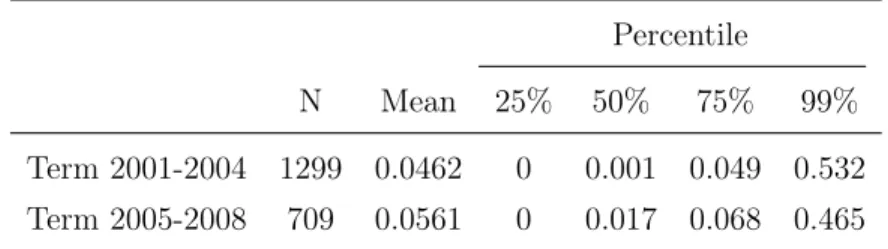
amount of misappropriated funds as a proportion of the total amount audited.19 This information is available for only 1,422 municipalities, as it was not possible to compute the amount of resources involved in some irregularities. The level of observation is the municipality-term, meaning that we can clearly identify the term during which electoral irregularities took place. In other words, if a municipality was selected in a lottery in 2007, it will likely appear in the sample twice, as the auditors checked spending that occurred in both the 2001–2004 term and the first part of the 2005–2008 term. We present in Table 1 the summary statistics of Corruption divide by electoral term.
We use candidates’ level of education as a proxy for quality. Specifically, we consider the minimum number of years necessary to attain a certain degree.20 Alternatively, we use the share of candidates that completed Mandatory School. The TSE provides data on the level of education of candidates for the city council. For each municipality, we distinguish between the Average Education level of candidates in the incumbent’s and the challengers’ coalitions. The incumbent’s coalition includes candidates from all the parties that run in the same coalition as the incumbent mayor’s party and who belonged to the winning coalition in the previous municipal election.21 The challengers’ coalition includes candidates running for all other parties. As an additional measure of quality we consider candidates’ job. That is, we associate to each candidate the average national salary correspondent to her profession and we compute coalitions’ Average Income.
Further, we compute the same variable considering new candidates (i.e., those who were not city councilors in the previous term) and re-running candidates. We also take into account the Median Education level of candidates and two other characteristics relevant for political selection – the Share of Female candidates and Average Age.22
We compute similar measures for mayoral candidates, but focus only on candidates belonging to the same party as the incumbent. Finally, we consider the Share of Seats
19In the original dataset this variable is called Broad Fraction of the Amount. Note that we do not
consider a binary measure of corruption as in the Brazilian context, the presence of corruption might not be informative per se, conversely we exploit the severity of the phenomenon. See Section 1 and the footnote 5.
20For candidates who started a degree but eventually dropped out, we assign half the number of years
that would be needed to complete it.
21We also show in Appendix Table A.4 our main results by defining the incumbent coalition as
composed of all parties that belonged to the winning coalition in the previous municipal election.
Won by candidates elected from the incumbent’s coalition.
We control for local political preferences by creating a dummy variable that equals 1 if the incumbent government was led by a mayor from Partido dos Trabalhadores, and 0 otherwise. This variable also controls for whether the municipalities is ruled by the same party in power at the federal government. The 2000 Brazilian Census provides data about the Population of the municipality, monthly per capita Income, Share of
Population Employed, the Gini Coefficient of income, the Share of population with a
Secondary Degree, the Share of Population in Urban areas, the share of population
working in different job sectors (Services, Transport, Public and Commerce). We also construct a dummy variableMedia, which accounts for the presence of local radio stations in the municipal area. This information is taken from the 2006 municipality surveyPerfil
dos Municípios Brasileiros: Cultura.
To provide homogeneous results in all our estimates, we apply a sequence of re-strictions to the original dataset on corruption provided by Brollo et al. (2013). First, we remove eight municipalities, as they did not yet exist in 2000 when the population census was conducted. Second, we consider only municipalities in which at least some parties support the incumbent’s coalition. Therefore, we remove 88 more municipalities. Finally, we exclude five municipalities in which there were no new candidates for city councilor (i.e., they were all incumbents). Clearly, by applying these restrictions the sample of municipalities we use in our analysis is no longer random. We address this issue in Section 7.
5. Estimation strategy
The main objective of this study is to test whether information shocks that change citizens’ voting behavior affect the quality of electoral candidates selected by parties. Specifically, we want to compare (1) the ability of candidates running for city council when the local government experiences an informative shock during the party selection period to (2) the ability of candidates running for city council in local governments that experience a similar informative shock at other points in time. In order to provide a reliable counterfactual analysis, we exploit the randomness of the timing of the disclosure of the audit reports to determine the group of Treated vs. Control municipalities.
To precisely determine the selection period (and hence the composition) of the two different groups, we identify two important dates in the electoral process. First, we
account for the deadline for parties to provide their candidate lists (i.e., July 5, 2004 for the elections held in October 2004 and July 5, 2008 for the October 2008 elections). Second, we consider the cutoff date for citizens to be affiliated with a party in order to run as a candidate for that party (i.e., October 3, 2003 for the October 2004 elections and October 5, 2007 for the elections held in October 2008). Thus, a municipality is considered to be treated if the disclosure of the report occurred between 12 to 3 months before election day. Indeed, depending on the lottery results, the communication of the audit reports might occur during, before or after what we identify as the treatment period. We think our definition makes clear that the focus on parties’ role in the selection process as the group of citizens willing to run for public office is mostly predetermined by the time the reports are disclosed.
It is worth noting that our strategy closely follows the one used in Ferraz and Finan (2008). However, as we are exploring a distinct research question, our definition of
treatment and the way we split the sample between treated and control municipalities
are rather different. Indeed, Ferraz and Finan (2008) define treated municipalities as those that received an auditing disclosure anytime before the election. Nevertheless, for the sake of completeness, we provide results where we use this latter definition of the treatment group. By doing so, on the one hand, we loosen the focus on parties’ role in the selection process as now the group of citizens that can become eligible to run for election is not predetermined. For example, citizens can decide to enroll in a political party as a response to an audit report published more than 12 months before the election, while this would not be taken into account with our primary definition of treatment. On the other hand, we control for the possibility that receiving a popularity shock in the three months before the election causes the withdraw from the electoral competition of previously selected candidates. For instance, political candidates from the incumbent political party that experience a very negative popularity shock might withdraw from the electoral competition so that the incumbent party may replace these candidates. Related to this point, we also report results where we exclude from the analysis municipalities that had the auditing disclosed more than 12 months before elections. We do so given that it is not straightforward to think of them as part of the control group as the informational
shocks occurred before the end of the selection period.23
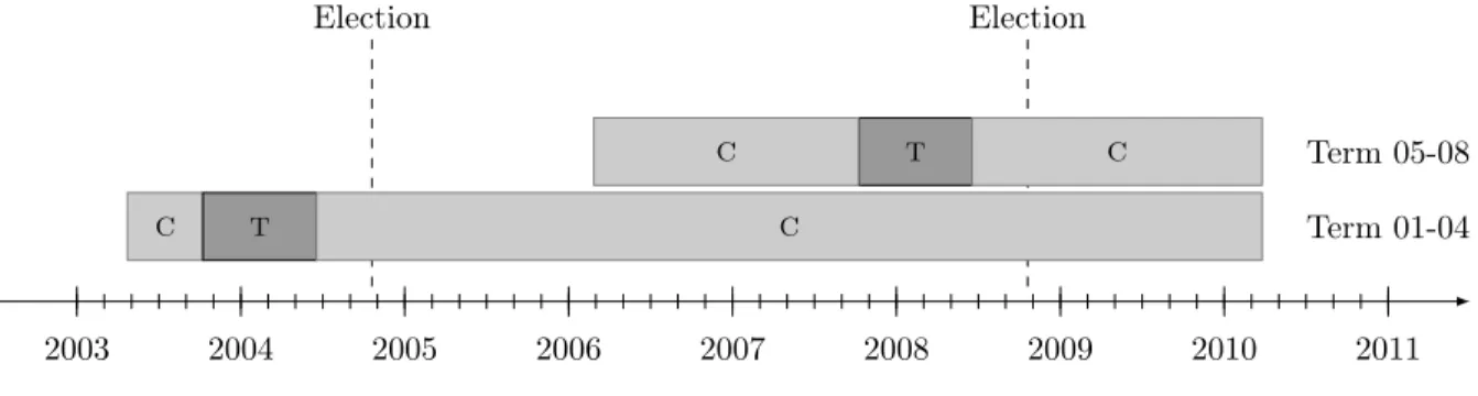
Another aspect to take into account is that auditing reports reveal a misuse of public funds that could cover both terms we include in our analysis. This could be a problem if it were not possible to determine the exact timing of the misbehavior. In this were the case, citizens would be limited in their judgment as it would be less clear who was accountable for the discoveries made during the audit. Luckily, the corruption data we use categorize the misuse of public funds by term and municipality, which allows us to identify the treated and control groups for each term as reported in Figure 1.
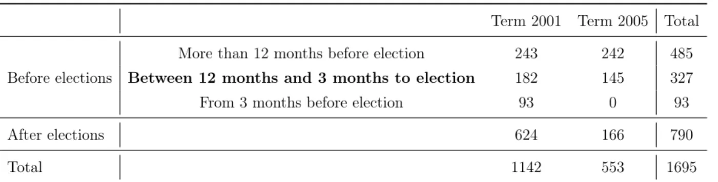
Table 2 summarizes the sample composition, differentiating accordingly to the time of the disclosure of the auditing report. Over the two terms, we have 1,695 observations. Following our main definition of treatment: 327 are treated (19.3% of the sample) and 1,368 are controls (80.7% of the sample).24 We have 182 treated and 960 control mu-nicipalities for the 2001–2004 term. Here, the treated mumu-nicipalities are the ones drawn from the four lotteries disclosed between October 2003 and April 2004, while the control group includes all municipalities selected in the other 25 lotteries that had audit reports released in the 2001–2004 term. For the 2005–2008 term we have 145 treated and 408 control municipalities. The treated municipalities were drawn from the three lotteries disclosed between January 2008 and June 2008, while the control group comprises all municipalities selected from the six lotteries disclosed between February 2006 and July 2007 plus the four lotteries disclosed between December 2008 and March 2010 that were audited for federal funds released in the 2005–2008 term.25
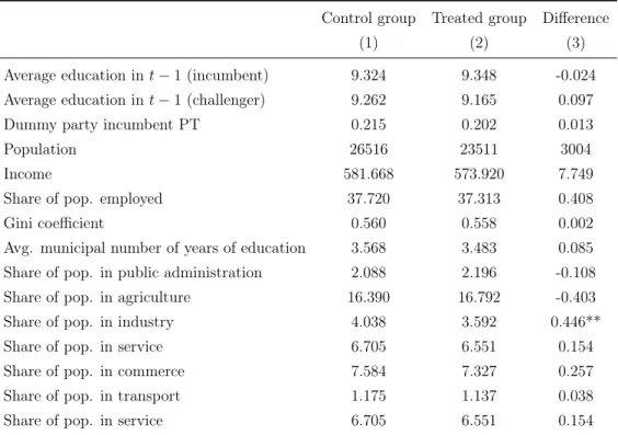
Table 3 reports the summary statistics for the two groups of municipalities. Indeed, although our sample is a sub-sample of those selected within the randomized lotteries, it seems well balanced. Only the share of the population working in the industrial sector 23In summary, the auditing disclosed more than 12 months before elections are used as part of the
control group in Table 4, as part of the treated group in Table 6 and excluded from the sample in Appendix Table A.3.
24Instead, if we consider the Ferraz and Finan’s (2008) definition we would have 905 treated
observa-tions (43.4% of the sample) and 790 as controls (46.6% of the sample).
25The reports disclosed before February 2006 did not account for funds released in the 2005–2008
term. 374 municipalities appear in the sample twice, as they are part of the control group for the first term and part of either the control or treated group in the second term. Municipalities that were audited more than once appear in our sample only with reference to the first draw. In this way, we avoid the possibility that the potential long-term effects of the audit would bias our estimates (Avis et al., 2017).
is different between the two groups at the 5% significance level. Note that including this variable in our specifications does not affect our findings.
Formally, we start the analysis by estimating the following ordinary least squares (OLS) model:
Yist=β Tist+δXi+γs+λt+ist, (1)
where i denotes the municipality, s the state and t the term. Yist can be the Average
Year of Schooling of either all or freshmen candidates for city councilor, from either
the incumbent or the challenger coalition. Tist is a dummy taking a value of 1 for municipalities with audit reports released during the selection period (i.e., from 12 to 3 months before the election), while Xi is a set of time-invariant municipal controls. Finally, γs are state-fixed effects, λt are term-fixed effects and is is the error term. We use an OLS model with standard errors clustered at the municipality level.
Thanks to the random assignment of the auditing among municipalities, the coef-ficient β is the causal parameter of interest. In other words, it represents the average effect of the release of the auditing reports on candidates’ education levels. State-fixed effects are included in all specifications, since the random assignment was stratified at the state level. Therefore, we ensure that our identification accounts for the heteroge-neous probability of selection on the treatment faced by municipalities from different states. In addition, term-fixed effects account for other unobservable characteristics that might have changed from one term to the next. We include municipal controls in order to provide more precise estimates in case the randomization still produces a selection of treated and controlled municipalities with unbalanced characteristics.
We expect the estimates from Equation (1) to produce significant results if the audit-ing disclosure per se matters in the candidate selection process, regardless of the actual information provided. However, this would only be the case if the information disclosed differs from what the voters or parties expect (Ferraz and Finan, 2008) – i.e., if there is a systematic under- or over-estimation of a municipality’s level of corruption.
Therefore, we refine our baseline analysis by taking into account the results of the auditing process. We produce different estimations to test whether the effect of the disclosure on the selection of candidates depends on the kind of information reported. Specifically, we estimate the following equation:
Yist=β1 Tist× Corruptionist+β2 Tist+β3 Corruptionist+δXi+γs+λt+ist, (2)
where Corruptionist is the share of corrupted resources. Moreover, to provide more flexible estimations and to account for potential non-linearity of the effects, we interact
T with a variable identifying municipalities that belong to different quartiles of the distribution of corruption. In other words, we compare the effect of the disclosure of different levels of corruption on the level of education of the pool of candidates. This is a crucial point because, depending on the level of corruption revealed, the information shock could send either a positive or negative message to citizens. However, using this approach could raise important issues if our measure of corruption simply serves as a proxy for other municipal conditions. We check for this possibility in Section 7.
6. Results
6.1. Baseline analysis
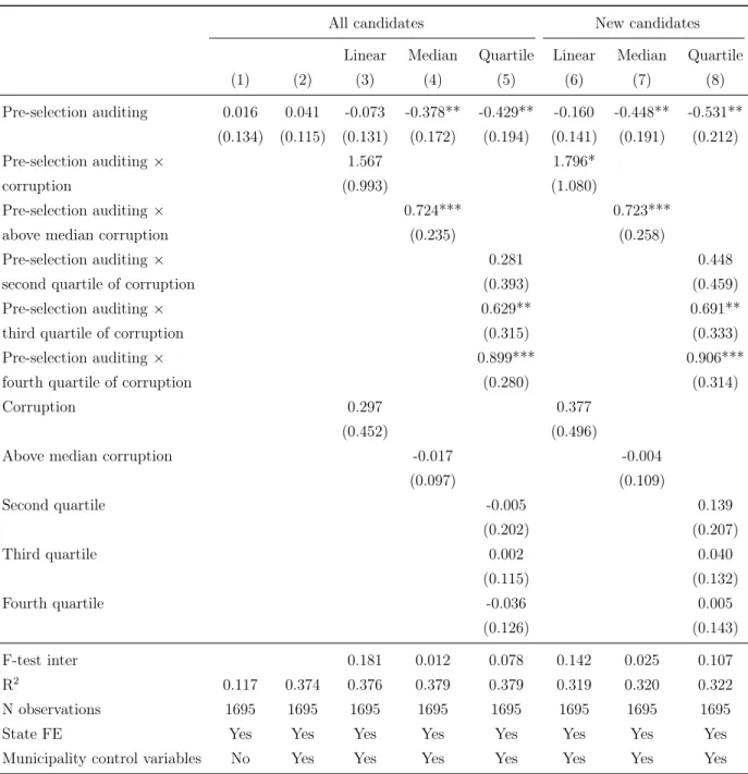
In this section, we report our central results. Specifically, Columns (1) and (2) of Table 4 show the results from the estimates of Equation (1), in which the dependent variable measures the level of education of all candidates in the incumbent’s coalition. As expected, the disclosure of reports per se has no direct effect on candidates’ qual-ity. Moreover, the inclusion of municipal covariates does not seem to have a sizable impact on the main coefficient, which is in line with a balanced sample thanks to the randomization of the treatment. The remaining columns of Table 4 report estimates of Equation (2). Columns (3) to (5) report the effect of the auditing, interacted with the level of corruption, on the education of all candidates selected by the incumbent coali-tion’s parties. Column (3) provides the first indication that reporting high corruption boosts the quality of candidates put forward by the incumbent’s party. The interaction term has a positive sign, but it is not statistically significantly different from 0. Column (4) reports the estimate where the treatment status variable interacts with a dummy that identifies whether a municipality is in the top 50th percentile of the distribution of our measure of corruption.26 This result, coherently with Column (3), suggests that
26The level of corruption in the median municipality was 0.5%. Note that our results are confirmed
when the audit report is disclosed during the selection period, in municipalities with low levels of corruption candidates from the incumbent’s coalition have around 4.5 months less of schooling (coeff. -0.378). However, if high levels of corruption are exposed, we observe an increase in the average education of slightly more than 4 months of schooling (coeff. 0.724-0.378 = 0.346). Both coefficients are statistically significant. Therefore, there are more than 8.5 months of education difference depending on the signal provided by the audit. This difference corresponds to about 30–35% of one standard deviation.27 The coefficients in Column (5) indicate the quartile of corruption and emphasize that the effect is stronger with higher levels of reported corruption.28 The last three columns suggest similar results once the focus is only on new candidates (i.e., those who were not previously on the city council). This is a crucial finding, as using new candidates rules out the possibility that the estimates rely on a mechanical effect coming from the direct consequences of the audit (e.g., if the audit led to the incarceration of involved 27Note that the magnitude of our findings is comparable with previous papers on political selection.
For instance, Daniele and Geys (2015) and Daniele (2017) estimate a change in politicians’ education due to mafia presence of about 35% of a standard deviation. Kotakorpi and Poutvaara (2011) find that a 35% increase in salary leads to a 5-percentage-point increase in candidates with high education. Baltrunaite et al. (2014) report a modest increase of 2-3 months in politicians’ education after the introduction of gender quotas.
28Appendix Table A.3 show that the results are similar if we only use as control those municipalities
that have the auditing disclosure after the selection period. Appendix Table A.4 provides the results of changing the definition of the incumbent’s coalition to include all parties that supported the mayor in the previous election, regardless of whether they do so in the following election. The results are similar, though the positive effect on the education of candidates running for office in highly corrupt municipalities is smaller than the one found with our standard definition of incumbent’s coalition. This does not change if we consider the extended sample which includes all the 1396 municipalities where there is at least one candidate representing the old incumbent’s coalition. Additionally, Appendix Table A.5 includes an alternative measure of schooling as a dependent variable – the share of candidates that completed Mandatory School. Our findings are confirmed. Specifically, the share of candidates that completed mandatory school decreases by 4.3 percentage points where low levels of corruption are found, and increases by about 3.5 percentage points with levels of corruption above the median. Further, in Appendix Table A.6, we show that our results are mainly driven by the candidates’ selection for the 2004 elections. Finally, note that our main findings do not vary depending on the level of electoral competitiveness. Specifically, the change in candidates’ ability is not significantly higher in close elections and neither in case the mayor is re-running for office or is facing term limits (results available upon request).
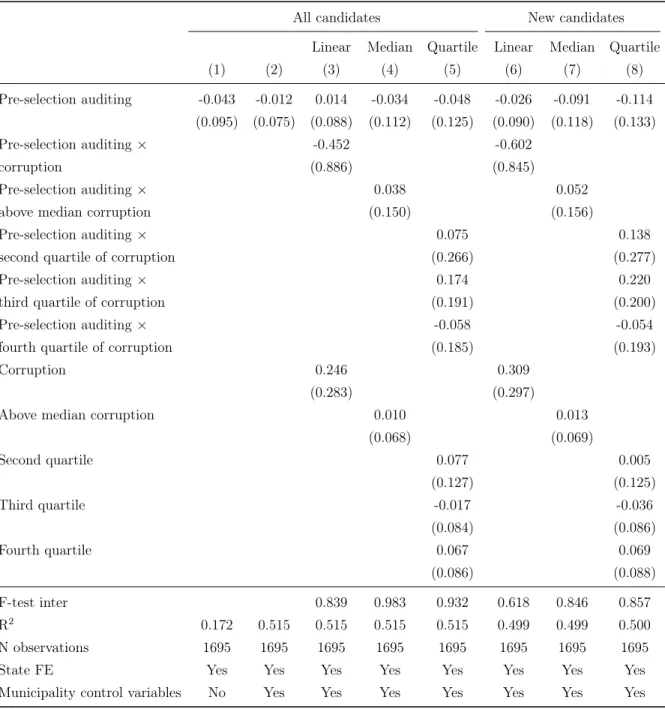
councilors who were mostly low-ability individuals).29 Table 5 shows that the challeng-ing coalition, which is not directly accountable for the outcome of the audit, does not change the education levels of its pool of candidates: the coefficients of interest are not statistically significant in any of the regressions.30 As suggested in Section 2, the effects of a popularity shock hitting the incumbent might spill to or have the opposite effect on the challenger. Therefore, these (lack of) results can be read in the light of the unclear nature of the shock received by the challenger.
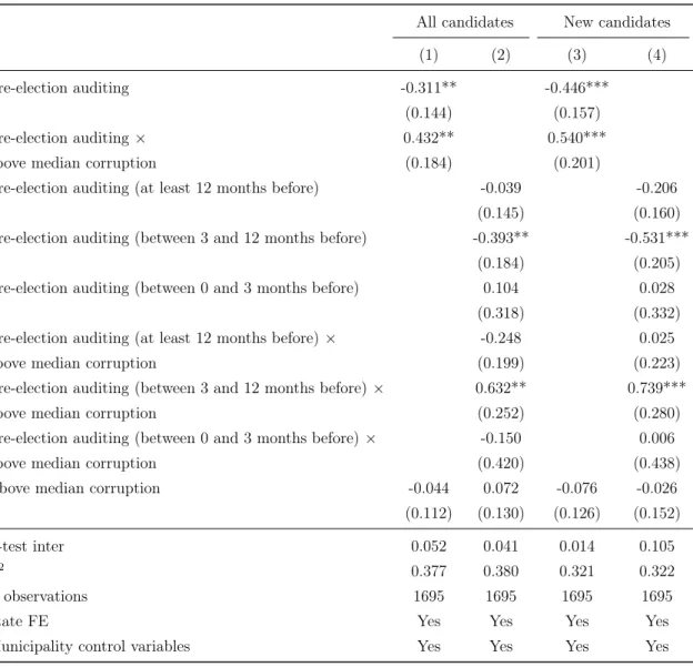
So far we considered a municipality to be treated if the disclosure of the report occurred during the selection period that we define taking places between 12 to 3 months before election day. However, one can still think of a more general definition of treatment period by considering as treated all municipalities that experience the disclosure of the report before the election. Therefore, following Ferraz and Finan (2008), we report in Table 6 the results from regressions where now the treatment includes the entire pre-electoral period.31 From Column 1 (all candidates) and Column 3 (freshmen), we still observe that audits reporting a low level of corruption lead to a worse political selection, while candidates’ ability increases in cities reporting above median levels of corruption. However, in the latter case, the magnitude of the estimated effect is lower than the one in Table 4. In Columns 2 and 4, instead, we separate the pre-electoral period in three parts: i) at least 12 months before the elections; ii) between 3 and 12 months before the elections; iii) between 0 and 3 months before the elections. It seems our results are driven uniquely by the period in between 3 and 12 months. Conversely, it appears that political selection does not change when the audit is released far from the elections (more than 12 months). Also, audits released just before the elections (less than 3 months) do not affect candidates’ selection. These results add credibility to our main definition of treatment.
Overall, our main result points to the effect of information on shaping the selection of political candidates. Given the institutional background of the case at study, our preferred interpretation of the empirical evidence is that political parties, rather than politicians, do react to the expected electoral shocks. On the one hand, they increase the 29Appendix Table A.7 provides results on re-running candidates. While the magnitude of the effect
is similar to the one estimated so far, this is barely significant.
30Our results are unchanged when considering the reaction of the most voted challenging coalition,
either in the previous or in the present elections.
quality of candidates in municipalities where elections become more difficult (i.e., where a severe report has been released) and they need to increase their popularity. This is in line with previous research showing that parties select better candidates when they need them, namely during more competitive elections (Galasso and Nannicini, 2011; Mattozzi and Merlo, 2015). Importantly, this intuition is supported by the suggestive results of Table A.1 and other more accurate studies showing that educated individuals are more likely to be elected (Dal Bó et al., 2017). On the other hand, elections become less risky when the local government experiences a positive shock, such as reporting no or little corruption. In this case, parties might decide to reduce the number of high-ability individuals if they are costly. For example, this is possible if the party shares rents with selected candidates, and this rent is higher the lower the public motivation (Besley, 2007), or if the party has to supplement candidates’ salaries, as high-ability individuals have a higher reservation wage (Mattozzi and Merlo, 2008). In our context, as highlighted in Table A.1, more educated candidates tend to receive a higher direct economical support from political parties.
Below, we propose additional analyses that complement the previous findings. We only report results that focus on parties that support the incumbent, as we have already shown the absence of effects for the challengers.
6.2. Additional analysis
6.2.1. A test on the role of political parties
Although we believe our results can likely be explained by parties’ strategic behaviors, we cannot rule out the possibility that they are also influenced by changes in the supply of politicians (i.e., the pool of individuals willing to run for office). This potential effect is already partially reduced because our treated municipalities cannot select individuals who are external to the party. In other words, the pool of potential candidates is pre-determined with respect to the treatment. Still, even within this sample of individuals, an effect could be expected. However, in principle, citizen–candidate models would predict results that are opposite to our findings (Caselli and Morelli, 2004; Osborne and Slivinski, 1996). For instance, one might expect high-ability individuals to have even lower incentives to enter politics after a political scandal. Similarly, it is hard to explain why high-ability candidates would refuse to stand for election in a municipality that appears to have a functioning administration, where it would be easier to be elected. Therefore, the effect of the disclosure of the audit report on individuals’ willingness to
enter politics will, if anything, adjust the size of our coefficients downward.
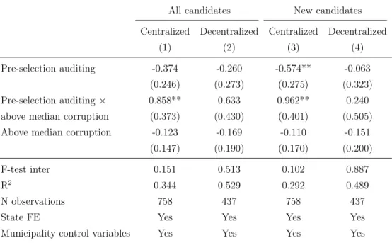
To provide additional support to our interpretation, we test the heterogeneity of the estimated effect with respect to the power structure of the mayor’s party. As explained in Section 3.2, in centralized parties top and mid-level party leaders are the decision-makers, while ordinary members have a greater voice in decentralized parties. Therefore, we expect that changes in the supply side of politicians would affect our results mostly when the popularity shock hits a decentralized party. In other words, it is easier for individuals who are willing to run for office to enter the pool of candidates of a decentralized rather than a centralized party.
We operationalize such a measure of party organization by following Guarnieri’s (2011) definition and consider parties to be decentralized if they are defined as pol-yarchic, and centralized if they are classified as either oligarchic or monocratic. We investigate the potential presence of a heterogeneous effect by splitting the sample into two groups depending on the incumbent mayor’s party of affiliation and running separate regressions.32 Table 7 presents the results from these regressions. In Columns (1) and (3) we consider municipalities governed by centralized parties (i.e., PSDB, PDT, DEM, PTB and PP), while in Columns (2) and (4) we use the sample of municipalities ruled by decentralized parties (i.e., PT and PMDB). The results tend to confirm our intuition. Indeed, we find a significant change in the education of the selected candidates only when the incumbent hit by the popularity shock was affiliated with a centralized party. Column (1) suggests that the presence of a positive shock decreases the quality of the pool of candidates by nearly 4 months of education (coeff. -0.374), though the coeffi-cient is not significant. A negative shock significantly increases the level of education by about 6 months of schooling (coeff. 0.858-0.374 = 0.484). Column (3) reports similar results for freshman candidates. In this case, a significant, though negative, effect on candidate quality is also observed for positive popularity shocks. In Columns (2) and (4), in which we limit the analysis to decentralized parties, none of the coefficient estimates is significantly different from 0. The signs are coherent with previous findings, but the coefficients are smaller in size.
32It is worth highlighting that the mayor’s party of affiliation in a given municipality is not randomly
6.2.2. Alternative dependent variables
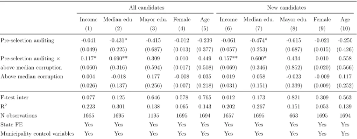
We first repeat our main analysis on a different measure of candidates quality. That is, instead of using candidates’ level of education we focus on candidates’ job (Besley et al., 2017). We estimated each candidate’s salary based on the average national salary of her profession, which we used to compute coalitions’ average salary. We used the logarithm of the average income of the incumbent coalition as the dependent variable. We report these new results in Columns (1) and (6) of Table 8. Both columns report very similar results: a negative popularity shock significantly increases the average income of the pool of candidates. The average income increase by 7.6% (coeff. 0.117-0.041=0.076) among all candidates and 9.6% (coeff. 0.157-0.061=0.096) in the sample of freshman. Hence our results are confirmed by this alternative measure of ability for the case of a negative shock. However, using this measure, we cannot confirm that a positive popularity shock affects candidates’ selection.
Second, we check whether the effect of the disclosure on candidates’ average level of education was driven by a general increase (or decrease) in the quality of the pool of candidates or whether it came from the selection of a few very good (or bad) candidates. Therefore, in Columns (2) and (7) of Table 8 we estimate Equation (2) by using the median level of education of candidates for city councilor as a dependent variable. The estimates reveal that the median level of education is also significantly affected, in the same direction as in the main analysis. In particular, the disclosure of a positive report decreases the level of median education by 5 months (coeff -0.431), while it increases by 3 months (coeff. 0.690-0.431=0.259) when the report is negative. The point estimates are similar when looking at freshmen candidates. This is consistent with a general change in the composition of the pool of candidates.
Third, we replicate the principal analysis looking at the education of mayoral can-didates. Therefore, the regression reported in Column (3) of Table 8 considers only municipalities in which the party of the incumbent mayor decided to present a candidate (either the incumbent mayor or a new candidate) in the next election. In Column (8) we focus on the sub-sample of new candidates. The main coefficients are not statisti-cally significantly different from 0, but their direction is consistent with the results for candidates for city councilors.33 The insignificant effect could be driven by two charac-teristics of the mayoral race that make the statistical test weaker. First, there is low
variability in the pool of candidates from one term to the next, as many mayors can run for re-election. This is not an issue if we look at the results in Column (8), which pertain to new candidates. Indeed, the effects are larger than those reported in Column (3) for incumbent mayors. The second characteristic that could be driving the insignifi-cant effect is the limited variability in the level of education of mayoral candidates: they are usually highly educated, particularly compared to the general population and city councilors (see Table A.2).
Finally, we explore the possibility that the disclosure might also affect other candidate characteristics – namely age and gender, which have been analyzed in previous studies on political selection (Esteve-Volart and Bagues, 2012; Daniele and Geys, 2015; Paola et al., 2010). We consider the average age of candidates and the share of female candidates as dependent variables. Our findings, reported in Columns (4 and 9) and (5 and 10) of Table 8, do not highlight any substantial change concerning these characteristics.34
6.2.3. Timing of the disclosure
In this section, we test the heterogeneity of the effect of the disclosure depending on when it occurred to determine whether the effect was mainly due to municipalities in which the audit report was released close to the end of the selection process. However, it could also be that audits released earlier have the strongest effect because the incumbent would have longer to change the selection of candidates.
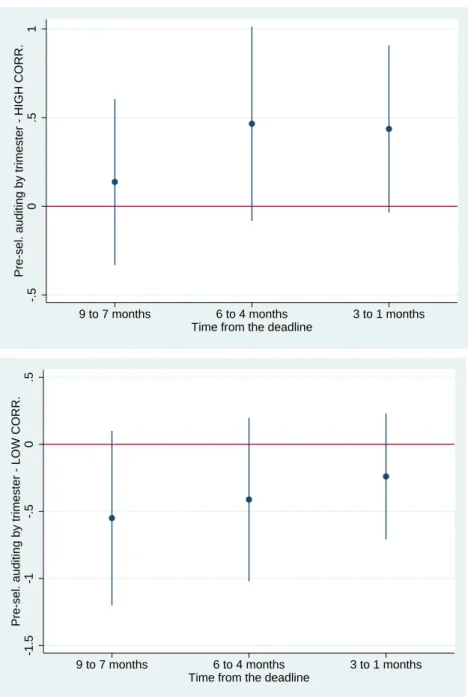
For this analysis we estimate the following regression separately for the sub-samples of municipalities with high and low corruption:
Yist = τ=3 X
τ=1
βτ Tist×1(t=τ) +δXi+γs+λt+ist, (3)
where Tist interacts with a set of dummies for each trimester of the treatment period. We report the results of these estimates in Figure 2. In the top panel we display point estimates and (95%) confidence intervals from a regression limited to the sample of municipalities in which audit reports revealed high levels of corruption, while in the bottom panel the analysis is constrained to municipalities with low levels of corruption reported in their audit.
34We also tested whether the disclosure affects the share of freshmen elected candidates. Also in this
While all coefficients are borderline insignificant, we can draw two interesting im-plications. First, the difference between the point estimates from the two groups of municipalities remains relatively stable over time.
Second, the level of education of the selected candidates is higher the closer to the election the report is disclosed. This is true regardless of the report’s severity. Thus, for instance, auditing disclosures that took place from 3 months to 1 month before the candidate list deadline had no effect on education when they revealed low levels of corruption, but had a large positive effect in municipalities with high levels of corruption. Hence, for a policy maker that aims at improving the overall candidates’ quality would be optimal to concentrate the auditing disclosure closer to the election. By doing so, it should avoid the unintended negative effect on candidates’ quality coming from the disclosure of positive reports occurred far from the election day.
6.2.4. Electoral results and local media
The mass media are the main channel through which citizens are informed about politicians’ behavior (Enikolopov et al., 2011). Indeed, the effect of a popularity shock on the electoral results varies depending on the availability and accessibility of sources of information (Ferraz and Finan, 2008; Costas-Pérez et al., 2012). If the results shown so far come from parties that act in anticipation of the potential impact of the audit report on the electoral results, we should also find that parties’ reactions depend on the presence of local media. Therefore, we expect audit reports to have a greater effect on the quality of candidates where citizens have easier access to information. To test this hypothesis, we follow Ferraz and Finan (2008) and account for the presence of local radio stations to characterize the different degrees of media penetration across municipalities. Therefore, we provide estimates by separately considering (1) municipalities that have at least one local AM/FM radio station and (2) municipalities with no local radio stations.35
Initially, we look at the impact of the audit reports on electoral outcomes. It is important to emphasize that this analysis adds to previous findings about the effect of the Brazilian auditing policy on electoral results since, to our knowledge, we are the first 35Similarly to what already discuss in section 6.2.1, media presence in a given municipality is not
to examine how the disclosure of corruption might also effect city council elections.36 Hence, we replicate the baseline model using theShare of Seats won by the incumbent’s coalition as a dependent variable. We first study the whole sample and then split it depending on whether municipalities have local radio stations. The results are reported in Columns (1), (2) and (3) of Table 9. The coefficients of interest are only significant when looking at municipalities where citizens have greater access to information. On the one hand, Column (2) shows that in municipalities where the disclosure of a positive report occurs during the selection period, the parties supporting the incumbent mayor win 5% more seats, while if the report is negative they win 5% fewer seats.37 On the other hand, Columns (1) and (3) suggest that, on average (and in the absence of a media presence) audits have very little effect on the electoral results. We can draw three important implications from these results. First, we can confirm that local media play an essential role in the accountability process. Second, the publication of the audit reports has a real effect on the election. This is a crucial element as in order for parties to react to the results of the audit report, they have to expect that voters care enough about the contents of the report to change how they vote. Third, voters still punish corrupt parties in elections even if they could select better candidates. Indeed, the electoral reward of a positive report is not affected by a potential decrease in the quality of candidates.
We then apply the same procedure to our baseline estimation. In Column (4) we report the same results as Column (4) from Table 4, while Columns (5) and (6) report the results for the samples of municipalities with and without local radio, respectively. In municipalities with radio stations, when the disclosure of the report provides a positive signal (i.e., low corruption) there is a decrease in the average years of schooling of all candidates of a bit less than 7 months (coeff. -0.582), while there is an increase in education of 3 months when the report provides a negative signal (coeff. 0.845-0.582 = 0.263). The coefficients are of a similar size when we consider either all candidates or only new candidates (Column 2). When we focus on municipalities with no local radio
36Ferraz and Finan (2008) show that corrupt mayors have a lower probability of being re-elected,
while Muço (2016) finds that voters also reduce their support of a corrupt incumbent mayor’s party in presidential elections.
37If we replicate this analysis and add to our treated municipalities those in which the report is
disclosed between the end of the selection period and election day, we have slightly different results. While the punishment for having a negative report is significant and of a similar magnitude, there is no electoral reward associated with receiving a positive report.
stations, Columns (3) and (4), the effect is either not significant or borderline significant and the reported coefficients are also smaller.
Overall, the results seem to be coherent with our intuition, as the effect of the audit report appears to be larger, and statistically significantly different from 0 at the 1% level, only in municipalities where citizens are likely to be more exposed to the media (i.e., those with local radio stations).38 Interestingly, the substantial change in the quality of the pool of candidates does not seem to be enough to significantly change the electoral results.39 These results are consistent with recent studies providing evidence that voters do not seem to be affected by ex-ante justifiable parties’ reactions to popularity shocks (Adam, 2012).
7. Identification checks 7.1. Sample selection
In our analysis we always constrain the sample to municipalities in which the incum-bent’s coalition decides to run for election. In other words, our sample is not random. This might produce a self-selection bias if the disclosure of the audit report affects the stability of the coalition and hence the decision to run for office. To account for this potential issue, we test whether there is any difference in the probability of being part of our sample between municipalities in which the auditing report was disclosed dur-ing the selection period (i.e., the treated group) or at other times (i.e., the control group). Therefore, we take the sample provided by Brollo et al. (2013), which includes all municipalities selected in the first 29 lotteries. From this larger sample we keep the municipalities used so far in the paper as well as those that were only excluded from the analysis because the incumbent party did not present any candidates. We then create a dummy variable equal to 1 if the municipality was part of our sample, and 0 otherwise. We replicate the same procedure for the sample used in the mayoral election analysis. The whole sample would be composed of 1,858 municipality-term observations, which 38We apply the same strategy by replicating the estimates in Table 8. The main findings do not seem
to be dependent on the presence of the media, except if the dependent variable is the median level of education; in that case, similarly to the results of this section, the effect appears to be more pronounced where local radio stations are available.
39In Appendix B we also provide results indicating the absence of an effect on the average quality of
excludes only 163 observations from the analysis. We report in Table 10 the formal test of the potential presence of self-selection bias, including a number of t-tests showing that being treated does not affect the average probability of being part of our sample. This is also true when we look separately at the samples with high and low levels corruption. In conclusion, this analysis suggests that a coalition’s decision to run for re-election is uncorrelated with the treatment, and that this is true for different levels of corruption.
7.2. Robustness of the corruption measure
Another potential concern about our identification is that our corruption measure may be serving as a proxy for other municipal features. In fact, while municipalities are randomly assigned to either a treated or control group, the level of corruption is not random and might depend on specific municipal conditions. For instance, corruption is potentially higher where there is extensive use of public investments, which usually occurs in bigger and richer cities. If this is true, we may be estimating how the release of an audit (regardless of its severity) has a differential effect on candidates’ education, for example in small vs. big or poor vs. rich cities. To help assess this potential issue, we replicate our baseline estimations and include additional interaction terms, where we multiply the treatment status dummy by a set of covariates that could be expected to be correlated with the level of corruption: Population, Income, Education
and Share of Pop. in Public Administration. The results, presented in Table 11, reduce
our concerns: in all the estimates, the interaction between the treatment status variable and the level of corruption is always significantly different from 0 and the coefficient is relatively stable across the different specifications. Moreover, the interaction terms that include the covariates never reach the conventional level of significance, whether analyzed in separate estimations (Columns 1 to 4) or jointly (Column 5).40 Overall, this suggests that our measure of corruption is unlikely to be proxying for other municipal characteristics.41
40We find similar results when the interaction term instead uses a dummy for the top 50% percentile
or dummies for the different quartiles.
41Note that in this table, while the interpretation of the interaction term "Pre-selection auditing X
above median corruption" does not change, the uninteracted coefficent "Pre-selection auditing" cannot be interpreted as in the previous tables, as in this case, we interact it with more than one variable in the same regression.