Multiscale multivariate functional principal component analysis with an application to multivariate longitudinal cardiac signals

(1)

MULTISCALE

MULTIVARIATE

FUNCTIONAL

PRINCIPAL

COMPONENT

ANALYSIS

WITH

AN

APPLICATION

TO

MULTIVARIATE

LONGITUDINAL

CARDIAC

SIGNALS

by

Andrew

N. Potter

B.A.,

Cornell

University,

2007

Submitted

to

the

Graduate

Faculty

of

the

Graduate

School

of

Public

Health

in

partial

fulfillment

of

the

requirements

for

the

degree

of

Doctor

of

Philosophy

University

of

Pittsburgh

(2)

UNIVERSITY OF PITTSBURGH GRADUATESCHOOL OF PUBLIC HEALTH

This dissertation was presented

by

Andrew N. Potter

It wasdefended on

December 2nd, 2016

and approved by

Stewart J. Anderson, PhD, Professor, Department of Biostatistics, Graduate School of Public Health, Universityof Pittsburgh

Robert T.Krafty, PhD,Associate Professor, Departmentof Biostatistics, Graduate School

of Public Health, Universityof Pittsburgh

Ying Ding, PhD, Assistant Professor, Department of Biostatistics, Graduate School of Public Health, Universityof Pittsburgh

Kehui Chen,PhD, Assistant Professor, Departmentof Statistics, DietrichSchool of Arts

and Sciences, University of Pittsburgh

Jeffery J. Teuteberg, MD, Associate Professor of Medicine, Heart and Vascular Institute, University of Pittsburgh Medical Center

Dissertation Director: Stewart J. Anderson, PhD,Professor, Department of Biostatistics,

(3)

Copyright c by Andrew N.Potter 2016

(4)

MULTISCALE MULTIVARIATE FUNCTIONAL PRINCIPAL

COMPONENT ANALYSIS WITH AN APPLICATION TO MULTIVARIATE

LONGITUDINAL CARDIAC SIGNALS

Andrew N. Potter,PhD

University of Pittsburgh, 2016

Abstract

Circadiancyclesinhumansareanimportanthealthindicatorincardiovasculardisease. With recent developments in ventricular assist devices (VADs), continuous recording of cardiac circadian cyclesin cohorts of heart failure patients is now possible for the entire life of the implant. Specifically, VADscontinuously record multivariatedata onblood flow and device status providing a unique longitudinalview of circadian cyclesin thesecohorts.

Ourstatisticalchallengeistosimultaneouslymodelthecohortaveragepumpoutput(PO) andpulsatility(PI)circadian cyclemeasurementsand patientspecificlongitudinalevolution ofhis/hercircadiancycle. While functionalprincipal componentsanalysis(FPCA)methods exist for the analysis of univariate longitudinal functional data with this structure, these techniques do not addressbivariate functionaldata.

We first divide time into two time scales: “fast” (circadian) and “slow” (longitudinal). We assume that the data are generated by smooth functions of time and extend FPCA to includebothtimescales. Useofamarginalmodel separatesthe estimationandinferencefor the two time scales. On the circadian time scale, we use wavelet based FPCA to estimate the cohort mean cycle and subject specific cycles. Confidence bands for the cohort mean and other estimates are calculated with a bootstrap. On the longitudinal time scale, a second FPCA step capturesthe subject specific longitudinal evolution. Furthermore, using datafromVADpatients,weimplementourmethod tocharacterize thepopulation circadian

(5)

cycle and identify regions of high between-subject variability in both the fast and slow time scales.

Our model provides a novel approach for analyzing multivariate circadian cycles. This work opens new avenues to understand the relationship between circadian cycles in simul-taneously recorded cardiovascular measurements. The public health significance is that care can be improved with better understanding of the longitudinal course of these patients.

Keywords: Functional Data Analysis, Discrete Wavelet Transformation, Marginal

(6)

TABLE OF CONTENTS

PREFACE . . . xi

1.0 INTRODUCTION . . . 1

1.1 RESEARCH QUESTIONS . . . 5

2.0 EXPLORATORY DATA ANALYSIS . . . 6

2.1 PERIODOGRAM ANALYSIS OF THE VAD DATA . . . 6

2.2 TIME DOMAIN EXPLORATORY DATA ANALYSIS . . . 8

3.0 CURRENT FPCA METHODS AND THEORY . . . 15

3.1 CROSS-SECTIONAL FUNCTIONAL DATA ANALYSIS WITH FPCA . . 15

3.2 THEORECTICAL SUPPORT OF FPCA . . . 17

3.3 LONGITUDINAL FUNCTIONAL DATA ANALYSIS WITH FPCA . . . . 19

3.3.1 Repeated Function FPCA. . . 20

3.3.2 Longitudinal Functional Principal Component Analysis . . . 21

4.0 CURRENT FPCA ESTIMATION ALGORITHMS . . . 23

4.1 ESTIMATION WITH A SPLINE BASIS. . . 23

4.1.1 Smoothing Parameter Estimation . . . 26

4.2 ESTIMATION WITH A TENSOR PRODUCT SPLINE BASIS . . . 27

4.3 ESTIMATION WITH A WAVELET BASIS . . . 28

4.4 CROSS-SECTIONAL FPCA ESTIMATION. . . 31

4.4.1 FPCA via smoothed covariance functions . . . 32

4.4.2 FPCA via smoothed eigenfunctions . . . 32

4.5 ESTIMATION OF RF-FPCA . . . 34

(7)

4.7 DETERMINING THE SIZE OF A FPCA THE BASIS . . . 35

5.0 NEW METHODOLOGY . . . 36

5.1 DEVELOPMENT OF THE MULTISCALE FRAMEWORK AND MODEL 36 5.1.1 Multiscale Decomposition and Marginal FPCA . . . 37

5.2 ESTIMATION AND INFERENCE . . . 40

5.2.1 Estimating the Average Circadian Cycles . . . 41

5.2.2 Slow Time Scale Estimation . . . 44

5.2.3 Selection of Number of Principal Components . . . 46

5.2.4 Bootstrap Confidence Intervals for the Fast Time Functions . . . 47

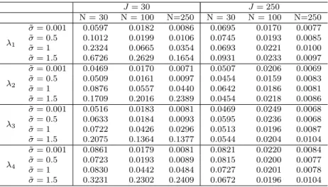
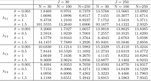
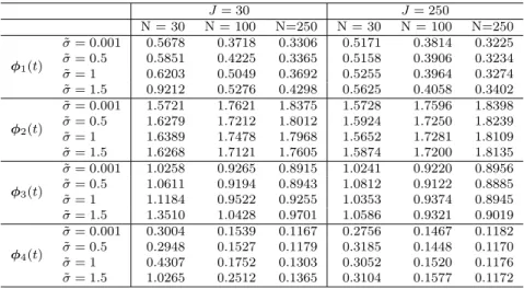
6.0 SIMULATION STUDIES . . . 48

7.0 VENTRICULAR ASSIST DEVICE WAVEFORM ANALYSIS . . . 57

7.1 APPLICATION OF MMFPCA . . . 60

8.0 DISCUSSION . . . 69

APPENDIX A. PLOTS OF VAD PATIENT RAW DATA . . . 71

APPENDIX B. ADDITION PERIODOGRAMS FOR VAD COHORT. . . 80

APPENDIX C. MATLAB CODE FOR FITTING MMFPCA . . . 88

(8)

LIST OF TABLES

1 1000 RMISE for simulated fast time mean with 128 fast time samples. . . 51

2 1000 RMISE for simulated fast time mean with 256 fast time samples. . . 51

3 RMSE for fast time eigenvalues simulated with 128 fast time samples. . . 51

4 RMSE for fast time eigenvalues simulated with 256 fast time samples. . . 52

5 RMSE for slow time eigenvalues simulated with 128 fast time samples. . . 52

6 RMSE for slow time eigenvalues simulated with 256 fast time samples. . . 53

7 RMISE for fast time eigenfunctions simulated with 128 fast time samples. . . 53

8 RMISE for fast time eigenfunctions simulated with 256 fast time samples. . . 54

9 RMISE for slow time eigenfunctions simulated with 128 fast time samples. . . 54

(9)

LIST OF FIGURES

1 Example VAD log file data. . . 3

2 Welch Periodogram from a representative patient showing circadian behavior. 8 3 Raw surface plot for 20 days of pump output for a representative patient. . . 10

4 Raw mean pump output circadian cycles for nine patients. . . 11

5 Raw mean puslatility circadian cycles for nine patients. . . 12

6 Raw mean pump output longitudinal evolution for nine patients. . . 13

7 Raw mean puslatility longitudinal evolution for nine patients. . . 14

8 The fast time scale basis functions for the simulation studies. . . 50

9 Heat map of pump output surface from one subject. . . 58

10 Surface plot of pump output surface from one subject. . . 59

11 Estimated VAD cohort average pump output and pulsatility. . . 61

12 Fast time eigenfunctions for the VAD cohort. . . 62

13 Slow time eigenfunctions for the VAD cohort. . . 63

14 Subject specific predicted pump output circadian cycle. . . 65

15 Subject specific predicted pulsatility circadian cycle. . . 66

16 The predicted patient specific pump output surfaces for VAD cohort. . . 67

17 The predicted patient specific pulsatility surfaces for VAD cohort. . . 68

18 Sample profile for 20 days of pump output and pulsatility for patient 2. . . . 72

(10)

26 Periodogram from patient 2. . . 80

27 Periodogram from pateint 3. . . 81

(11)

PREFACE

As with any large project or anything worth doing, my dissertation research has been a long and winding journey. The completion of this journey would not have been possible without the support of those around me. First I would like to thank my guide on this journey, my advisor, Dr. Stewart Anderson, who has provided essential support at every step along the way. My committee members, Dr. Robert Krafty, Dr. Jeffrey Teuteberg, Dr. Ying Ding, and Dr. Kehui Chen, have each provided expert guidance to improve the quality of my dissertation. I would also like to thank Dr. Jonathan Holtz, Dr. Robert Kormos, and Dr. Jeffrey Teuteberg who each provided the clinical touch to my dissertation and keep my research grounded in clinical relevance. One of the joys of a statistician’s job is the ability to collaborate with people with different backgrounds and viewpoints. I would like to provide a special thanks to Dr. Jonathon Holtz for providing the clinical data and motivations for which this project would not have been possible. I enjoyed developing as a student with him and exploring the possibilities of medical research. I would like to thank Dr. Joyce Chang for providing guidance during teaching and providing an area that makes it not only possible to meet with clinicians, but to form lasting collaborations with doctors.

I would also like to thank for emotional support of my family and friends who provided essential support during the process. My parents provided warm meals and an essential break when I felt overwhelmed during this process. The last person I would like to thank my fianc´e, Michelle, for providing me with support through the process, especially copy editing my dissertation, and helping me achieve my goals.

(12)

1.0 INTRODUCTION

Multivariate cardiac signals measured over a circadian (daily) cycle are frequently encoun-tered in the study of the long term health of heart failure patients. In previous chrono-biological studies, both blood pressure and heart rate show circadian variation in healthy humans (Millar-Craig et al., 1978; Lombardi et al.,1992;van de Borne et al., 1992; Takeda and Maemura,2011). In cardiovascular disease (CVD), including all types of CVD from mild hypertension to end stage heart failure (HF) and myocardial infarction (MI), disruption of the circadian cycle is associated with both increased risk of CVD as well as a symptom of CVD itself (Millar-Craig et al., 1978; Lombardi et al., 1992; Takeda and Maemura, 2011). During recovery from a MI, the amplitude of circadian variation in heart rate is depressed (Lombardi et al., 1992). The same pattern is seen in both heart rate and blood pressure circadian cycles in HF patients. Van de Borne et al. (1992) demonstrate that a blood pres-sure circadian cycle returns to normal in heart transplant patients within seven months post transplant. Due to the recent increase in use of left ventricular assist devices (VADs), a need for understanding the circadian cycles in these patients has arisen.

A VAD is a life-saving medical device consisting a pump implanted in a patient’s chest (Slaughter et al., 2010). Blood flows into the pump through an inflow cannula in the left ventricle and out into the ascending aorta and to the rest of the body. Blood is pumped using a continuously spinning impeller pump. The blood flow depends on both the pump speed and the patients heart function.

With the appearance of continuous logging of multiple device and hemodynamic param-eters (power, pump output [PO], pulsatility [PI], speed) in modern VADs, the ability to simultaneously study the daily evolution of the circadian cycle in these variables becomes possible. The two variables of clinical interest here are PO and PI. PO is a measure of

(13)

blood flow through the VAD. PI is a measure of blood flow variability. In patients with a VAD, both the characteristic shape and longitudinal evolution of the circadian cycles in PO, PI, and power are hypothesized to be important markers of long term health (Slaughter et al.,2010;Suzuki et al.,2014). However, no studies have yet linked this circadian variation to health outcomes. In one of the earliest studies of circadian cycles in VADs, Slaughter et al. (2010) shows that a circadian cycle in VAD power is present in VAD patients by end the of the first month post implant. Suzuki et al. (2014) report monthly variation in VAD power circadian cycle parameters such as amplitude and phase. These studies have analyzed changes in the circadian cycle by comparing an estimated parameter or sample means across several time points. Despite this recent research, the clinical meaning of these cycles in VAD patients is poorly understood.

As part of a larger study of circadian waveform behavior and its continuous longitudinal evolution in VAD patients, we propose a new functional data analysis method, multivariate multiscale functional principal component analysis (MMFPCA). Analyzing a small pilot dataset, our goal is to formulate answers to the clinical questions about a cohort of patients with VAD data such as: “Does a circadian cycle exist for VAD patients?” “If so, what is its shape?” “How do PO and PI jointly vary across a day?” Our pilot data consist of VAD clinical log files for nine patients sampled from a larger database at a major academic medical center. Each log file contains bivariate measurements of PO and PI recorded every 15 minutes for the entire life of the VAD implant. Data are downloaded at clinic visits but contains missing periods as data is only stored for 30 days before being over written. In our cohort, the length of follow-up ranged from 20 to 79 days after gaps were excluded.

Example data from a single patient are presented in Figure 1. This figure shows 20 days of data on the PO and PI waveforms with visually strong and correlated circadian cycles. For this patient, the daily minimum of PO is about 5000 mL/min, and the daily maximum is over 7000 mL/min. Similarly, the PI circadian variation ranges from 4000 mL to 9000 mL.

Appendix A contains plots of the remaining eight patients. Circadian variation is seen in the other patients.

(14)

2 4 6 8 10 12 14 16 18 20 days 5000 6000 7000 8000 mL/min Pump Output 2 4 6 8 10 12 14 16 18 20 days 2000 4000 6000 8000 mL Pulsatility

Figure1:ExampleVADlogfiledata.

(15)

Traditionally, the data are often analyzed using spectral or frequency domain methods such as periodograms and extensions. In the study of circadian cycles (chronobiology), the cosinor model, a parametric model that assumes the circadian cycle takes on a cosine shape, is often used. An excellent review byRefinetti et al. (2007) covers both the spectral analysis and cosinor approach in depth. While frequency domain approaches are briefly covered, this dissertation focuses mainly on the analysis of the functional aspects of our motivating data. Our statistical approach begins by viewing the VAD data as noisy observations on mul-tivariate functions of the two scales of time, the important features of these data occur over two independent time scales: the circadian cycle defining a “fast” time scale,t, and its longi-tudinal evolution defining a “slow” time scales. However, the data are originally collected as a function, F₍_τ₎_, _{of a single time variable,} _τ,_{requiring a transformation onto the two time} scales, (t, s). We introduce a novel statistical framework to jointly model both fast and slow time scales and the multivariate structure by modeling F₍_τ_{) using a function} _F₍_t_{) for the} fast time cycles that is repeatedly observed over a range of days. The longitudinal evolution over s is modeled with a functionG(s). This multiple scale approach was motivated by the two time solution method used in solving non-linear ordinary differential equations (ODE) (Fink et al., 1974; Strogatz, 1994). This framework formalizes the intuitively appealing approach dividing a continuously recorded signal into one period long blocks.

Instead of the challenging estimation of F₍_τ_{) for the entire cohort, the multiple time} scale changes the estimation problem to the tractable analysis of repeated observations of

F(t). Several recent papers address the modeling of repeatedly observed functions. These methods are based on the functional extension of principal component analysis, FPCA, which models random functions using an empirical basis function expansion. The longitudi-nal functiolongitudi-nal principal component alongitudi-nalysis (LFPCA), introduced by Greven et al. (2010), models the repeatedly observed functions using the FPCA equivalent of a linear mixed model, the longitudinal evolution is required to be linear. Park and Staicu (2015) extend LFPCA to the case when the longitudinal evolution follows an unknown function. This approach is effective when the longitudinal follow-up information is sparsely observed. LFPCA is one specific model that uses the marginal FPCA approach discussed in Chen et al. (2016). Another approach is repeated function functional principal component analysis (RF-FPCA)

(16)

introduced byChen and M¨uller(2012). RF-FPCA models the univariate repeated functional observations by correlated conditional FPCA for each time unit of longitudinal follow-up. RF-FPCA also uses a non-parametric form for the effect of longitudinal time.

In order to model our VAD data, LFPCA and RF-FPCA must be both extended to multivariate observations that are densely sampled on both fast and slow time scales. Ac-cordingly, our proposed method is inspired by RF-FPCA’s approach for dense longitudinal data and LFPCA’s marginal decomposition of the covariance structure (Chen et al., 2016;

Park and Staicu, 2015; Greven et al., 2010). The marginal covariance model is used as a starting point as it easily extends to the multivariate case, unlike the conditional covariance model used in RF-FPCA.

1.1 RESEARCH QUESTIONS

The following research aims will be addressed in this dissertation:

1. Develop a multivariate functional principal component analysis (MFPCA) to analyze the daily cyclic and long term behavior of a population of VAD patients when all patients show a daily cycle.

2. Characterize the performance of the new method using large sample theory and finite sample simulation studies.

(17)

2.0 EXPLORATORY DATA ANALYSIS OF THE VENTRICULAR ASSIST DEVICE CIRCADIAN PATTERNS

In this chapter, we present results from an exploratory data analysis of the waveforms seen in the ventricular assist device (VAD) data presented in Figure 1. Throughout this chapter, consider the sample grid for each patient τℓ with ℓ = 1,2, . . . , n×Ji. Here, n is the total

number of samples per day and Ji is the numbers of that each patient i is observed. Our

exploration of the patterns in the VAD clinical log files consists of using periodograms to search for signals with a period of one day. Also, we break both PO and PI into day long blocks. Then, surface plots of the raw data aid the visualization of any circadian pattern, and its longitudinal evolution. In addition, both the daily marginal patient specific means and the marginal patient specific longitudinal evolution are examined.

2.1 PERIODOGRAM ANALYSIS OF THE VAD DATA

Because one of the motivating clinical questions is to characterize the presence of a circadian pattern in the VAD patient population, we use a periodogram to examine the strength of any periodic signal in each patients data. At each frequency,ωg,a periodogram ˆPi(ωg) represents

the sample amplitudes of sine and cosine functions oscillating at ωg (Shumway and Stoffer, 2011). If a patient has a circadian cycle, a strong peak is expected a 1 cycle/day.

(18)

Unless the circadian cycle is represented by a pure cosine signal, peaks at the higher order harmonic frequencies will also be present. A harmonic frequency is any frequency that is an integer multiple of fundamental frequency, 1 cycle/day, in our case. Visual examination of the harmonics aids in deciding if spectral analysis of repeated functional data analysis is appropriate for out VAD data.

As ˆ_Pi(ωg) is an inconsistent estimate of the power spectrum, a smoothed estimate is

needed. In our case, we used a Welch periodogram, which smooths ˆ_Pi(ωg) by sub-setting

F_i₍_τ_ℓ_{) into non-overlapping blocks (}_Welch_,₁₉₆₇_{). Then a periodogram is estimated for each} block. Finally, these are averaged together yielding a smoothed estimate.

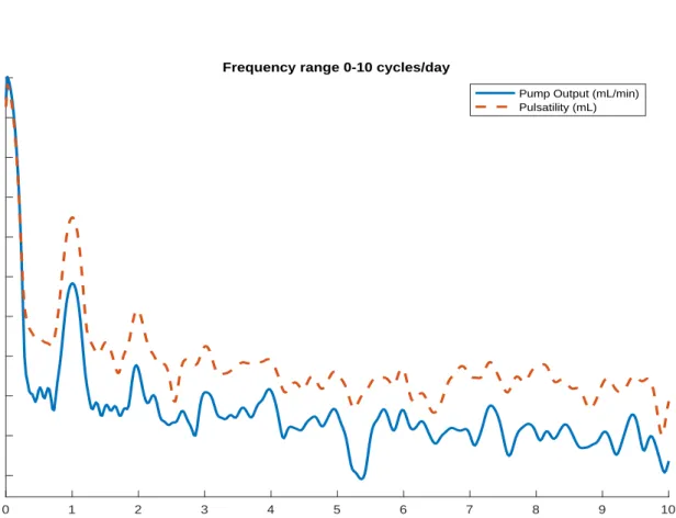
The Welch periodograms of PO and PI are shown in Figure2for a representative patient. Additional periodograms for the other eight patients can be found in Appendix B. In Figure 2, a peak at 1 cycle/day in both PO and PI shows that both PO and PI have a circadian cycle. As the periodogram contains significant peaks at harmonics of 1 cycle/day, the circadian cycle has a shape that cannot be accurately captured as a linear combination of only sine and cosine functions with daily periods. Additionally, an increase of power (_≈80 dB) in the very low frequency end of the spectrum indicates that the random process is likely non-stationary. The other eight patients show a similar pattern.

(19)

0 1 2 3 4 5 6 7 8 9 10 Frequency (cycle/day) 35 40 45 50 55 60 65 70 75 80 85 Power/Frequency (dB/cycle/day)

Frequency range 0-10 cycles/day

Pump Output (mL/min) Pulsatility (mL)

Figure 2: Welch Periodogram from a representative patient showing circadian behavior.

2.2 TIME DOMAIN EXPLORATORY DATA ANALYSIS

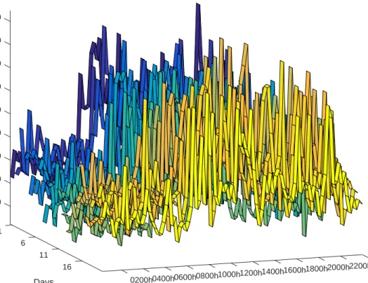
As each patient has a circadian cycle, the data is now split into non-overlapping day long blocks. Figure3 presents 20 days pump output plotted in one day long blocks for the same patient as in Figure 1. In Figure 3, different colors represent different days. For this patient, circadian variation is seen in each seen for all 20 days. Also, we observed that the average PO is lower during the days 10-15 than during the first ten days or last five days. Figure 1

also shows that measurement error has two major regimes (low during sleep and high during the day). Therefore, level-dependent noise is present in the data.

Even without any smoothing, both the circadian cycle and its longitudinal evolution can be simultaneously visualized. The PO circadian cycle consists of two potentially smooth regions, sleeping and waking, with an abrupt change during the morning hours. Examining

(20)

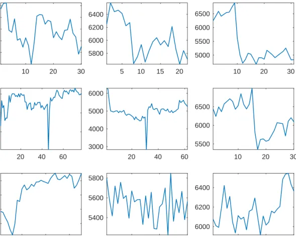
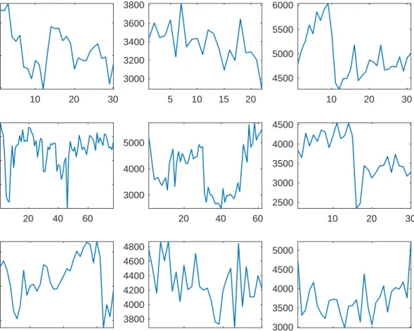
the patient’s raw average circadian cycles for both PO and PI, see Figures4and5, circadian variation is clearly seen in all patients. While there may exist a smooth circadian cycle for any patient, abrupt jumps are seen in most patients, e.g., the time period from 0700h-1100h in the bottom center patients shows a rapid increase in PO, then decrease. The PI circadian cycle, see Figure 5, shows a similar and mostly likely correlated pattern. Also, all patients have a rapidly changing PO and PI during the morning wake-up period. Outside of this period, the PO and PI levels change slower. In Figures 6 and 7, each days average PO or PI is plotted against calendar day. In the top left plot of Figures 6 and 7, both PO and PI are seen to decline from their highest level at day 1 to their lowest level at day 12. During these 12 days, PO declines by approximately 1000 mL/min and PI by 2000 mL. Then both sharply rebound by day 15. Several other patients show day-to-day fluctuations of a similar magnitude. In contrast, the plots in the lower right show little longitudinal variation in flow. Therefore, we focus on introducing estimation that are able to model functions with multiple types of smoothness and does not fail is the presence of non-white noise. Several candidate estimation techniques include the use of wavelet basis functions and varying band-width smoothers. We use wavelet basis functions throughout the rest of this dissertation to address these features of the data as the use of a wavelet basis has better performance in data with regions of rapid and slow variation.

(21)

4500 5000 5500 6000 1 6500 7000 7500 8000 mL/min 8500 6 Pump Output Days 11 0000h 2200h 16 2000h Hours 1800h 1600h 1400h 1200h 1000h 0800h 0600h 0400h 0200h

(22)

5 10 15 20 5000 5500 6000 5 10 15 20 5200 5400 5600 5800 6000 6200 6400 5 10 15 20 4500 5000 5500 5 10 15 20 5400 5600 5800

Pump Output (mL/min) ₅ ₁₀ ₁₅ ₂₀

4600 4800 5000 5200 5 10 15 20 5500 6000 6500 5 10 15 20 Hours 5400 5500 5600 5700 5 10 15 20 Hours 5000 5200 5400 5600 5800 5 10 15 20 Hours 5500 6000 6500

(23)

5 10 15 20 4000 5000 6000 7000 5 10 15 20 2500 3000 3500 5 10 15 20 4000 4500 5000 5500 5 10 15 20 3500 4000 4500 5000 Pulsatility (mL) 5 10 15 20 3500 4000 4500 5 10 15 20 2500 3000 3500 4000 5 10 15 20 Hours 2900 3000 3100 3200 5 10 15 20 Hours 3000 3500 4000 4500 5 10 15 20 Hours 3000 4000 5000

(24)

10 20 30 5200 5400 5600 5800 6000 6200 5 10 15 20 5800 6000 6200 6400 10 20 30 5000 5500 6000 6500 20 40 60 4000 5000 6000

Pump Output (mL/min) ₂₀ ₄₀ ₆₀

3000 4000 5000 6000 10 20 30 5500 6000 6500 10 20 30 Calendar Day 4500 5000 5500 6000 10 20 30 Calendar Day 5400 5600 5800 10 20 30 Calendar Day 6000 6200 6400

(25)

10 20 30 4000 5000 6000 5 10 15 20 3000 3200 3400 3600 3800 10 20 30 4500 5000 5500 6000 20 40 60 3000 4000 5000

Pump Output (mL/min) ₂₀ ₄₀ ₆₀

3000 4000 5000 10 20 30 2500 3000 3500 4000 4500 10 20 30 Calendar Day 2500 3000 3500 10 20 30 Calendar Day 3800 4000 4200 4400 4600 4800 10 20 30 Calendar Day 3000 3500 4000 4500 5000

(26)

3.0 CURRENT FPCA METHODS AND THEORY

Before reviewing the existing FPCA methods, we introduce several important sampling schemes on both the fast and slow time scales. On the fast time scale, all methods discussed and developed assume that the data points are equally spaced and have the same number of samples each day. Therefore, the observed fast time data points form a dense regular grid tl with l = 1, . . . , n. The slow time sampling can take on several types of sampling.

It is worth exploring four different types of longitudinal sampling encountered in LFD. If we denote each repeated observation time of sij for the ith subject, sij’s fall into one of

several main cases. The first case is dense regular follow-up where the sij are sampled for

all values of j _∈[0, Ji]. In this case, each subject can have the same length of follow-up, i.e., J1 =J2 =· · ·=JN =J (balanced design) or unbalanced follow-up with no missing data. In

both of the these cases, the total number of observations,N_×JorP_iJi diverges asJi → ∞.

A third case is dense regular follow-up with missing data. Alternatively, the follow-up can have sparse irregular sampling with subjects having different lengths of follow-up Ji and

random gaps between each sij. Here, P_iJi < ∞ as Ji → ∞. Equipped with the sampling

schemes, we now embark on an overview of existing FPCA techniques for both cross-section (single observation) functional data and longitudinal (repeated observation) functional data.

3.1 CROSS-SECTIONAL FUNCTIONAL DATA ANALYSIS WITH FPCA

Before illustrating analysis of longitudinal FPCA, we overview FPCA for a single observation of univariate or multivariate functions on N subjects. We term this analysis cross-section FPCA to distinguish it from longitudinal or repeated FPCA. The observed data consist of

(27)

functionsyi(t) observed oni= 1, . . . , N subjects at equally spaced time pointstl =t1, . . . , tn.

For example, a study may be interested in asking what is the population average VAD PO curve during the first day post hospitalization and how PO varies betweens patients.

These data are modeled assuming that they are generated by a smooth function and observed with noise (Ramsay and Silverman, 2005). Therefore, we start all FDA with the model

yi(t) =Fi(t) +ǫi(t), (3.1)

where Fi(t) is a subject specific random function with mean function µ(t) and covariance

function_K(t, t′₎_,_{and noise process}_ǫ

i(t).Defining centered subject specific random functions

as Xi(t) = Fi(t)−µ(t), the covariance function is the expectation of product of centered

random functions, K(t, t′_{) = cov(}_X i(t), Xi(t′)) =E Xi(t)Xi(t′) . (3.2)

This formulation leads to the model

yi(t) =µ(t) +Xi(t) +ǫi(t). (3.3)

At the observed time points tl, Ramsay and Silverman (2005) argue that the sample

mean vector ˆ µ(tl) = 1 N N X i=1 yi(tl) (3.4)

and sample covariance matrix

ˆ K(tl, tl′) = 1 N ₋1 N X i=1 yi(tl)−µˆ(tl) yi(tl′)−µˆ(t_l′) (3.5)

are reasonable but noisy estimators for the population mean and covariance. These estimates are used in FPCA. As both (3.4) and (3.5) still contain noise, a regularization step is included in FPCA. While the data can be pre-smoothed, we recommend that regularization takes place during FPCA to both prevent over-smoothing and reduce to the computational burden. Details of several smoothing procedures are discussed in Chapter 4.

In this dissertation, all unknown functions such as µ(t) can be accurately represented by a basis function expansion. If φp(t) form a set of P orthogonal basis functions on the

(28)

a random functionXi(t) has the approximate expansionXi(t)≈PPp=1ξipφp(t) where the ξip

are random basis coefficients. If the basis functions are known functions such as B-splines or trigonometric functions, the coefficients are estimates using techniques such as smoothing or p-splines, kernel density estimators, or wavelets, see Ramsay and Silverman (2005). If the basis functions are unknown, FPCA is used to determine a set of basis functions that minimizes the square error of the approximation of ˆXi(t). As FPCA forms the basis of

several important LFDA methods, we provide an in-depth review of FPCA.

The condition of least square approximation error implies that a FPCA basis can be found using the least square objective function, (Ramsay and Silverman, 2005). For a population of N subjects, the objective function is

H = N X i=1 kXi(t)−Xˆi(t)k22 = N X i=1 Xi(t)− ∞ X p ξipφp(t) 2 2 , (3.6)

where_{k · k}2 is theL2-norm for functions defined onL2. This norm has the integral represen-tation

kXi(t)k22 =

Z T

Xi(t)2dt,

for a function Xi(t) defined on a domain, T. Ramsay and Silverman (2005) show that the

set of basis functions that minimizes (3.6) has the additional property that it maximizes the amount of variation explained in the random functions Xi(t).

3.2 THEORECTICAL SUPPORT OF FPCA VIA THE

KARHUNEN-LO`EVE THEOREM AND MERCER’S THEOREM

The theoretical support for FPCA is the Karhunen-Lo`eve expansion and Mercer’s theorem (Happ and Greven, 2015). Mercer’s theorem allows for the eigen-decomposition of a covari-ance function _K(t, t′_{) into eigenvalues} _λ

(29)

that _K(t, t′_{) is square integrable, Mercer’s Theorem states that} K(t, t′_{) =} ∞ X p=1 λpφp(t)φp(t′), (3.7)

with the eigenvalues and eigenfunctions being solutions to

Z

T K

(t, t′)φp(t′) dt′ =λpφp(t). (3.8)

When Mercer’s theorem holds, the Karhunen-Lo`eve theorem states that a random function has a basis expansion

Xi(t) = ∞ X

p=1

ξipφp(t), (3.9)

where the basis coefficient or principal component (PC) scores are

ξip = Z

T

Xi(t)φp(t) dt (3.10)

with ξip ∼ N(0, λp) that are uncorrelated for different p. For a subject i, the predicted

response function is

yi(t) =µ(t) + X

p

ξipφp(t).

For multivariate functions, the case when yi(t) consists of D simultaneous observations

instead of 1 observation, analysis the mean functionµ(t) is unchanged and is conducted in a component-wise fashion. However, analysis of multivariate random functions Xi(t) requires

an adjustment to the covariance function _K(t, t′₎_, _{Karhunen-Lo`eve theorem and Mercer’s}

theorem. For multivariate data, the covariance function changes to

K(t, t′_{) =}_E_X

i(t)Xit(t′)

. (3.11)

Accordingly, the eigenfunctions from equations (3.7) and (3.9) change to φp(t).However,

the eigenvalues and the PC scores remain scalars. This small change in the theory will cause challenges in FPCA estimation, discussed in Section 5.2.1. These theorems provide a firm foundation for the creation of a data driven basis set that has minimal least square approximation error.

(30)

3.3 LONGITUDINAL FUNCTIONAL DATA ANALYSIS WITH FPCA

Often, the function of interest is observed not just once, but repeatedly observed over multiple days, weeks, years. For example, the VAD power circadian cycle is recorded for each day that the patient has a VAD implanted. Therefore, we introduce both how functions are observed longitudinally and detail theory and application of two useful existing models: LFPCA and RF-FPCA. While both LFPCA and RF-FPCA are able to analyze longitudinal functional data (LFD), they differ in approach, interpretation, and computing time.

Both methods start with the idea that the LFD form a two-dimensional surface on the domain (t, s). They model the cohort mean surface µ(t, s) and provide two different FPCA models for the random functionsXi(t, s). For both RF-FPCA and LFPCA, the basic model

for LFD when both t and s are continuous variables is

yi(t, s) =Fi(t, s) +ǫi(t, s)

=µ(t, s) +Xi(t, s) +ǫi(t, s), (3.12)

where yi(t, s) are the observed data, Fi(t, s) is a random surface with mean surface µ(t, s)

and mean zero subject specific surface Xi(t, s) =Fi(t, s)−µ(t, s) with covariance function

K(t, t′_{, s, s}′_{) = cov}_X

i(t, s), Xi(t′, s′), and ǫi(t, s) is the error which is specified for each

model. In (3.12), the random functions have a two dimensional Karhunen-Lo`eve expansion

Xi(t, s) = ∞ X

p=1

ξipφp(t, s) (3.13)

where φp(t, s) are the eigensurfaces of

K(t, t′_{, s, s}′_{) = cov}_X i(t, s), Xi(t′, s′)= ∞ X p=1 λpφp(t, s)φp(t′, s′) (3.14)

with eigenvalues, λ1 > λ2 >· · ·> λ∞. The PC scores are found with the double integral ξip = Z S Z T Xi(t, s)φp(t, s) dtds.

(31)

Conducting FPCA on the full covariance, _K(t, t′_{, s, s}′₎_, _{is challenging as a four dimensional}

smoothing step is required. Instead both RF-FPCA and LFPCA conduct a two step analysis of the covariance.

As the mean surface is estimated by well accepted techniques, both LFPCA and RF-FPCA focus on modeling the random processesXi(t, s),see details in Section4.2. RF-FPCA

models the conditional stochastic processes Xi(t|s) with a set of conditional FPCA models

that depends upon the longitudinal observation. These expansions and the associated basis functions are dependent on longitudinal time. The longitudinal dependence in theXi(t|s) is

modeled through a second stage FPCA. In contrast, LFPCA uses a longitudinally constant set of basis functions for Xi(t, s) with the longitudinal dependence induced through time

varying coefficients, ξip(sij) when sij form a sparse sample (case 4).

3.3.1 Repeated Function FPCA

Chen and M¨uller (2012) model Xi(t|s) by a two step Karhunen-Lo`eve expansion instead

where the function X(t, s) is observed repeated for fixed s leading to the conditional repre-sentation X(t_|s). For the ith _subject,

Fi(t|s) =µ(t|s) + ∞ X

p=1

ξip(s)φp(t|s) (3.15)

where for fixed s, φp(·|s) are the eigenfunctions of the covariance function K(t, t′|s) =

covX(t_|s), X(t′

|s)and ξip(s) are the corresponding PC scores which are random functions

of s with mean zero and varξip(s)=λp(s) for fixed s.

Now a second Karhunen-Lo`eve expansion is applied to theξip(s) representing these

func-tions as ξip(s) = ∞ X q=1 ζiqpψqp(s) (3.16)

whereψqp(s) are the “second level” eigenfunctions and the mean zero ζiqp are “second level”

PC scores. The associated covariance operator has kernel_K(s, s′_{) = cov}_ξ

ip(s), ξip(s′)

.

(32)

Then, they combine the Karhunen-Lo`eve expansions in Equation (3.15) and Equation (3.16) leading to the final model

Fi(t|s) = µ(t|s) + ∞ X p=1 ∞ X q=1 ζiqpψqp(s)φp(t|s) (3.17) =µ(t_|s) + ∞ X p=1 ∞ X q=1 ζiqpϕqp(t|s)

where ϕqp(t|s) = ψqp(s)φp(t|s). The surfaces, ϕqp(t|s),describe how the FPCA basis varies

over time.

In order to use the model in (3.17), we need to both truncate the infinite sums as well as estimate a smooth mean function, ˆµ(t_|s), and covariance functions ˆ_K(t, t′

|s). Chen and M¨uller (2012) recommend setting the size of each FPCA basis is determined using fraction of variance explained (FVE), although both AIC and BIC also give reasonable results. The estimation of the mean and covariance depends upon both the sampling in both t and s.

Chen and M¨uller (2012) assume that sampling in the t₋direction to be on a dense regular grid. All cases of longitudinal sampling can be analyzed with RF-FPCA by changing the FPCA algorithm.

3.3.2 Longitudinal Functional Principal Component Analysis

When the subjects have sparse longitudinal sampling, LFPCA can be used instead of RF-FPCA. In contrast to RF-FPCA, LFPCA uses a longitudinally constant set of basis functions,

φp(t), with time varying coefficients, ξip(sij), where sij are the subject specific longitudinal

observations, (Park and Staicu,2015;Greven et al.,2010). Park and Staicu(2015) introduce a modified version of (3.12) for sparse follow-up:

yi(t, sij) =µ(t, sij) +Xi(t, sij) +ǫi(t, sij), (3.18)

where all terms are defined as previously but evaluated at the time pointssij.However, the

random functions, Xi(t, sij),have different Karhunen-Lo`eve expansion,

Xi(t, sij) = ∞ X

p=1

(33)

with a marginal covariance_K(t, t′_{) =} R R _K₍_{t, t}′_{, s, s}′_{) d}_s_d_s′_._{Chen et al.}₍₂₀₁₆_{) refers to this}

type of covariance kernel as a marginal kernel. Using the same strategy of a double FPCA, the full LFPCA model is

yi(t, sij) = µ(t, sij) + ∞ X p=1 ∞ X q=1 ζiqpψqp(sij)φp(t) +ǫi(t, sij), (3.19)

where ψqp(sij) are the eigenfunctions of the longitudinal covariance function

Kp(sij, s′ij) = X q λqpψqp(sij)ψqp(s′ij), ζiqp = Z ξip(sij)ψqp(sij) ds,

ǫi(t, sij) is the error term, and all else is defined as previous. In any application, the infinite

sums are truncated using FVE or another method.

As these models consist of three parts, mean function (surface), a random function for the domain_T, and a longitudinal random function on _S,the estimation methods considered in Section 4.4 are broken down in the same fashion. For both RF-FPCA and LFPCA, the mean surface estimation and both FPCA estimation steps are estimated with existing algorithms. However, both methods introduce new techniques to handle the estimation of the ξip(s). These topics are the focus of the next Chapter.

(34)

4.0 CURRENT FPCA ESTIMATION ALGORITHMS

In Chapter 3, we introduced several models for analyzing longitudinal functional data and the theoretical backing. Before any of these techniques are useful for analyzing data, an estimation procedure is needed. This chapter consists of three main sections: function esti-mation with a spline basis, function estiesti-mation with a wavelet basis and FPCA estiesti-mation. Splines are introduced as they are commonly used and necessary for understanding exist-ing techniques. In addition, wavelets are introduced as they are used for the estimation algorithm of the new method, see Chapter 5.

4.1 ESTIMATION WITH A SPLINE BASIS

A popular functional estimation approach for estimating an unknown function such asµ(t) uses a B-spline basis. We first discuss spline estimation for functions of one domain variable before moving on to functions of two domain variables and tensor product splines. In this section, we discuss estimation of a mean curve µ(t) of data Yi(tl) = µ(tl) +ǫi(tl) observed

on i= 1, . . . , N subjects and at time points tl where l = 1, . . . , n. Here, ǫi(t) are mean zero

normally distribute random variables. The covariance structure is discussed separately for each estimation method.

B-spline basis functions are a set of known polynomial functions, eg(t), of degreem with

compact support that form an orthonormal basis for L2 on an interval [t0, tmax] (de Boor, 1972; Schumaker,2007). To represent a function µ(tl) observed at time points tl ∈[t0, tmax]

(35)

using a spline basis, first partition of [t0, tmax] intoG intervals such that each interval is

Ig = [tg, tg+1), g = 1,2, . . . , G+ 1.

The points, tg, are called knots, and successive basis functions are joined at a knot ( Schu-maker,2007). The basis functions,eg(tl),havem−1 continuous derivatives. Using a B-spline

basis, a smooth function such as µ(t) is represented by

µ(t) =

G X

g=1

ageg(t), (4.1)

where ag are the basis coefficients, eg(t) are B-spline basis functions, and G is the number

of functions.

The first step in estimating (4.1) is to select the number and location of the knots must be determined. One option is to pick a small number of knots yielding a very smooth estimate of µ(t). However, this approach fails to capture interesting behavior of the data. To make sure that the data are well described, a knot can be placed at every time point tl for a

total of n knots. However, this approach may lead to the over-fitting of the data with the estimated function ˆµ(tl) passing through every ¯Yi(tl) =

P

iYi(tl)

N . To prevent this over-fitting,

some type of regularization or penalty on the size of the spline coefficients must be used. Two common types of penalties are continuous penalties, often on the second derivative, that lead to smoothing splines and discrete or differencing penalties, often on the second difference, that lead to the P-spline solution (Ramsay and Silverman,2005;Eilers and Marx,

1996). Both of techniques penalize have a similar effect to penalize the fit if the estimated function ˆµ(tl) has a large global curvature measure.

To fit this spline model of the data, the least squares objective function in Equation (4.3) is minimized with respect to the coefficients ag in (4.1)

SSE= 1 N N X i=1 n X l=1 " Yi(tl)− G X g=1 ageg(tl) #2 (4.2)

Following the approach of Ramsay and Silverman (2005), equation (4.2) is re-expressed in matrix notation SSE = 1 N N X i=1 (Yi−EA)t(Yi−EA), (4.3)

(36)

where Yi is a data column vector, E is a matrix of basis functions, and A is a matrix of

coefficients. The weighted least squares criteria can also be used if the error structure is believed to not be i.i.d normal with a covariance matrix, Σ, leading to the addition of a weight,W =Σ−1, to (4.3), SSEw = 1 N N X i=1 (Yi−EA)tW−1(Yi−EA).

The smoothing spline model is a common choice for fitting (4.3). A smoothing spline sets the number of basis functions equal to the number of observations, G= n, and places a knot at each time point tl. If this model is directly applied to (4.3), this spline model is

over-parametrized as the number of basis coefficients equals the number of data points. To prevent over-fitting of the model, roughness penalties are incorporated into the least squares objective function (Silverman, 1985). The penalized least squares criteria is

SSEP EN = 1 N N X i=1 (Yi−EA)tW−1(Yi−EA) +λAtDA (4.4)

Here, λ is a smoothing parameter that controls how much impact the penalty term AtDA

has on the fit and D is a matrix of derivatives of eg(tl). Often the 2nd derivatives are used

leading to a cubic smoothing spline model. When λ= 0, the spline fit by (4.4) interpolates the data, and when λ _{→ ∞}, the spline fit by (4.4) is a linear least squares regression of the dataY.(4.4) has the effect of shrinking the coefficientsag towards a linear fit while allowing

for important curvature in µ(t). Ramsay and Silverman(2005) provide a solution to (4.4) in terms of a smoothing matrix

S(λ) = E EtW E+λD−1EtW. (4.5) For observations, Yi,the underlying smooth function µ(tl) is estimated by

ˆ µλ =S(λ) 1 N N X i=1 Yi.

Notice that ˆµλ is still a function of the unknown smoothing parameter λ. Estimation of ˆλ

depends on the type of error processǫi(tl). We consider two types of error structures, white

(37)

4.1.1 Smoothing Parameter Estimation

Since all of the above estimation techniques depend on a tuning parameter,λ, the parameter must either be set by hand or estimated from the data using a pre-specified criterion. As manual control of the tuning parameter is impractical, automated techniques are used. These techniques are based on minimizing the mean square error (MSE) E_kµˆλ(tl)−µ(t)k=ǫi(tl)

for the spline estimation. An estimate ˆλ that minimizes the MSE is considered optimal. If the error processǫi(tl) is assumed to be a white noise process, the MSE can be estimated

using the leave one observation out cross validation estimator (CV). The CV estimator of the MSE is CV(λ) = 1 N N X i=1 1 n n X l=1 Yi(tl)−µˆ( −l) λ (tl) 2 = 1 N N X i=1 1 n n X l=1 Yi(tl)−µˆλ(tl) 2 1₋S(λ)ll 2 , (4.6)

where ¯yl is the observed data and ˆµ(λ−l)(tl) is the estimated value of the ˆµestimated without

the lth _{observed point (}_{Hastie et al.}_,₂₀₀₉_;_Gu_,₂₀₁₃_).

The quantity in (4.6) can also estimated by generalized cross-validation (GCV) intro-duced by Craven and Wahba (1979). Unlike CV score, GCV is invariant to orthonormal transformations of the data (Gu, 2013; Craven and Wahba, 1979). The GCV criteria is a function of the smoother matrix S(λ) and for n points is computed by

GCV(λ) = 1 N N X i=1 nY_it[I ₋S(λ)]2_Y i tr[I₋S(λ)] 2 . (4.7)

Because (4.7) only depends on the trace of S(λ),the GCV score is slightly more efficient to compute than the CV score. GCV smoothing parameter estimation assumes that the ǫi(tl)

are independent and identically distributed mean zero normal random variables, ǫi(tl) ∼ N(0, σ2_{). GCV fails in the case of colored noise because} _ǫ

(38)

4.2 ESTIMATION WITH A TENSOR PRODUCT SPLINE BASIS

In the analysis of longitudinal functional data, an important step is the estimation of the unknown mean surface, ¯y(t, s) = µ(t, s) +ǫ(t, s). Basis functions of t and s are needed. One choice is the thin-plate spline (TPS); however, the penalty that leads to the TPS is complicated and time intensive to evaluate for bivariate splines, and practically intractable in higher dimensions. Therefore, the tensor product spline basis is introduced represent functions of multiple variables. A tensor product spline represents µ(t, s) by observed on a regular grid in t, s by

µ(t, s) = X 1≤g≤G

1≤h≤H

ag,heg(t)eh(s) (4.8)

whereeg(t) are theGB-splines in thetdirection,eh(s) are theH B-splines in thesdirection,

andag,gare the spline coefficients (Xiao et al.,2013). Similar to the single variable smoothing

case, a penalized estimation procedure is used to prevent over fitting. The fitting criteria is

1 N N X i=1 n X l=1 J X j=1 " yijl− G X g=1 G X g=1 ag,heg(tl)eh(sj) #2 + Pen(λt, λs), (4.9)

where the first term is the multiple variable sum of squares and the second term is a multi-variable penalty term (Park and Staicu, 2015). Any penalty consists of at least at direction penalty and a s direction penalty (Xiao et al., 2013; Park and Staicu, 2015). In Park and Staicu (2015), they use a t₋direction penalty

Pent=λt Z Z ∂2_µ₍_{t, s}₎ ∂t2 dtds

and a s₋direction penalty

Pens=λs

Z Z _∂2_µ₍_{t, s}₎

∂s2

dtds.

Alternatively,Xiao et al. (2013) introduce the sandwich smoother, a multivariable extention of P-spline smoothers Eilers and Marx (2003); Xiao et al. (2013). P-splines differ from smoothing splines as the penalty matrix is directly calculated as the 2nd _{difference of the}

(39)

surface, first define ¯Y = 1

N PN

i=1yijl as the data matrix. Xiao et al. (2013) proposes to

estimate

ˆ

µ=StY S¯ s= (Ss⊗St) ¯Y (4.10)

where

Sk=Ek(EktEk+λkDtkDk)−1Ekt

is smoother matrices for thekth _{direction, ¯}_Y _{is the data matrix,} _D

k is a differing matrix of

order mk,⊗ is the tensor product, and all other terms defined as previous. For two domain

variables, this formulation leads to the penalty term

P =λtEstEs⊗DttDt+λsEttEt⊗DtsDs+λtλsDtsDs⊗DttDt.

By minimizing

kY¯ ₋EtAEskF2 + vec(A)tPvec(A),

where the norm is the Frobenius matrix norm,Xiao et al.(2013) introduced a fast algorithm for estimating ˆµ(t, s). The smoothing parameters are selected using GCV.

While smoothing splines and P-splines are commonly used for FDA, we do not use them as basis functions for the analysis of our VAD waveform data because of the noise structure and regions of rapid change. Our exploration of splines provides a gentle introduction into functional data analysis with basis functions that is expanded in the discussion of wavelets. Additionally, these spline estimators are used in LFPCA and explanation of LFPCA esti-mation is clarified by a clear understanding of both smoothing and P-splines.

4.3 ESTIMATION WITH A WAVELET BASIS

Another important class of basis functions is the wavelet multi-resolution basis. A wavelet basis differs from the spline basis in Section 4.1 in that it has two types of basis functions that capture the behavior µ(tl) at multiple resolutions. Scale functions eg(tl) at scale level g describe the average behavior of µ(tl) and wavelets egh(tl) that reflect the variation at

(40)

We illustrate a wavelet basis using Haar wavelets inspired by the approach of Nievergelt

(2001).

On the interval [0,1), the father Haar wavelet is defined as

e[0,1)(t) =      1 if 0_≤t <1 0 o.w. . (4.11)

Nievergelt (2001) extends this definition to a half-open interval of arbitrary length 1/g on thegth _{scale. For}_g _{= 2}_,_{these intervals form a partition}_P

2 =0,1/2,1 of [0,1). Therefore, the Haar scale functions for Pg are defined by

eg(t) =      g if (h₋1)/g _≤t < h/g 0 o.w.

for h = 1,2, . . . , g. At the gth _{scale, the scale functions approximate a function} _µ₍_t_{) on}

[0,1/g) by its average value

µ∗

g =g

Z h/g

(h−1)/g

µ(t)eg(t) dt.

While the scale functions capture the average of µ(t), they ignore any changes in µ(t) on the interval h on the gth _{scale. Wavelet functions capture the change in} _µ₍_t_{) for the} _hth

interval on the gth_{. The Haar wavelet,}_e

gh(t), is defined as

egh(t) =e[(h−1)/g,(h−1)/g+1/2g)(t)−e[(h−1)/g+1/2g,h/g)(t). (4.12)

The change in µ(t) at scale g and location h is

µ∗

gh=g

Z h/g

(h−1)/g

µ(t)egh(t) dt. (4.13)

By constructing wavelets for any scale g, a Haar Wavelet basis can be constructed to ap-proximate µ(t) to any desired detail level. While Haar wavelets are the simplest wavelets, many other wavelet functions exist. Two important wavelet bases are Daubechies wavelets and Daubechies’ least asymmetric wavelets, “symlets” (Mallat, 1999). These wavelets do not exist in closed form but can be calculated recursively. In addition, the coefficient vector,

µ∗

(41)

The basic plan for wavelet estimation of an unknown function is to first use the discrete wavelet transform (DWT). The DWT transforms a vector of data ¯Y from the time domain into the wavelet basis functions defined above (wavelet domain) via a linear transformation,

¯

Y∗ =WY¯ (4.14)

where W is the transform matrix defined by the integral transformation in (4.13) and ¯Y∗

is the vector of wavelet coefficients. When the ¯Y are modeled as noisy observations of an unknown function, µ(tl) with errors ǫ(tl), the wavelet domain model is

¯

Y∗

gh=µ∗gh+ǫ∗gh

where µ∗

gh is the vector of wavelet coefficients for the unknown function, ǫ∗gh is the wavelet

transform of the noise, and all else is defined as previous (Johnstone, 2013). Assuming that ǫ_∼ N(0,Σ), it is easily seen that ǫ∗

∼ N(0,WΣWt₎_. _When _Σ₌ _σ2_I_, _{Donoho and}

Johnstone (1995) show that the coefficient ˆµ∗

gh is estimated well with a threshold estimator, η( ¯Y∗

gh, ̟). A threshold estimator keeps all ¯Ygh∗ that are large and sets all other ¯Ygh∗ following

a threshold rule. Many types of thresholds exist in the literature; however, we focus on the soft threshold, ηS( ¯Ygh∗, ̟) = sgn( ¯Ygh∗)(|Y¯gh∗| −̟)+, and the hard thresholdηH( ¯Ygh∗, ̟) =

¯

Y∗

ghI(|Y¯gh∗| ≥ ̟). Here, sgn(·) takes on the sign of its argument, (·)+ is non-zero when its argument is positive, and I(_·) is the indicator function.

Several techniques estimate ˆ̟ from the data. The universal threshold ˆ̟U = ˆσ√2 logn

is the simplest choice. However, ˆ̟U requires the noise to be i.i.d. normal. A more general

threshold rule is derived using Stein’s unbiased risk estimator (SURE) (Donoho and John-stone, 1995; Johnstone and Silverman, 1997). The SURE method is based on finding the ˆτ

that minimizes mean square error and selects the value ˆ̟ that minimizes

ˆ H(̟) = ˆσ2n+X g X h ( ¯Y_gh∗,2_∧̟2)₋2ˆσ2I_{|Y¯_gh∗_{| ≤}̟_} (4.15) and ˆ ̟ = arg min ˆH(̟). (4.16) ˆ

(42)

In the presence of colored noise, Johnstone and Silverman(1997) modifies (4.16) to have a different threshold at each wavelet decomposition level, g. Colored or non-white noise is any case when Σ₆=σ2I.For example, the soft threshold estimator takes the form

ˆ

µ∗

gh =η( ¯Ygh∗, ̟g) = sgn( ¯Ygh∗)(|Y¯gh∗| −̟j)+, (4.17)

where ̟g is the threshold at the g scale, and all else is defined as previous. Johnstone and Silverman (1997) adjust the threshold such that

ˆ

̟g =σg̟ˆ( ¯Yg∗/σg)

for the levels in the specific wavelet decomposition. The modification of the threshold is the only adjustment needed for using a wavelet threshold estimator with colored noise because threshold estimation is a coordinate-wise operation (Johnstone and Silverman,1997).

4.4 CROSS-SECTIONAL FPCA ESTIMATION

Estimation algorithms for FPCA fall into one of two categories: those that smooth the estimated covariance function, ˆ_K(tl, tl′), or those that smooth the eigenfunctions, ˆφ_p(t_l).

Since both methods are used in the estimation of our new methods, we discuss both. The estimation algorithms are introduced assuming that ǫi(tl) ∼ N(0, σ2I). In each case, we

comment on the robustness of each algorithm to violations of the white noise assumption as physiological signals often violate the white noise assumption.

(43)

4.4.1 FPCA via smoothed covariance functions

This section follows the approached for covariance smoothed FPCA outlined in Yao et al.

(2005). Recalling from (3.5) that

f K = (N ₋1)−1 N X i=1 XiXit

is a raw estimate of _K(tl, tl′) at the observed times t_l with the column vector X_i = X_i(t_l).

Here, Xi(tl) = yi(tl)− µˆ(tl). Because E(Kf) = K + σ2I, Yao et al. (2005) recommend

estimating the smoothed covariance ˆK by replacing the diagonal elements Kll with ˇKll =

1/2 Kl−1,l+Kl,l+1,where theKl−1,l andKl,l+1are the nearest off diagonal elements. At this point, ˇKllhaven−2 elements lacking elementsK11andKnn.Therefore, linear extrapolation

is used to calculate these elements. Any surface estimator such as the sandwich smoother is used to smooth the matrix, ˜K,to yield a smoothed estimate, ˆK.

Because ˆK is a discretized estimate of_K(t, t′₎_,_{the integral eigenvalue equation (}_3.8_{) with}

a matrix eigenvalue equation

ˆ

Kφp =λpφp, (4.18)

where ˆK is a discrete version of smoothed covariance,φp is the pth eigenfunction evaluated

at the same points as ˆK, and λp is the pth eigenvalue. Ramsay and Silverman (2005) state

that (4.18) can be solved using any matrix PCA or eigenvalue software. However, the results must be converted back to the functional data form using interpolation. This approach to FPCA is relativity straight forward to implement provided that ˆK is easy to estimate. In the case of white noise, this is true. However, if this step is challenging such as with non-white noise error structures or non-smooth regions of _K(t, t′_{), it is more fruitful to apply}

regularization to the eigenfunctions instead.

4.4.2 FPCA via smoothed eigenfunctions

While many methods exist for FPCA with smoothed eigenfunctions, seeRamsay and Silver-man (2005), we focus attention on adaptive sparse PCA (ASPCA) introduced by Johnstone and Lu (2009) both for computation efficiency and robustness to violations of white noise

(44)

and smoothness in the eigenfunctions. These are always concerns in physiological signal analysis. Considering a covariance matrix, K, with eigenvectors, φp, and eigenvalues, λp,

ASPCA estimates theP eigenvectorsφp by transforming the PCA algorithm from the data

basis where K is not sparse to one where K∗ = W KWt is sparse, where W is a trans-formation matrix. Orthonormal basis vectors, eg, represent both the data Xi and PCs as: Xi =P_gXg,i∗ eg,whereXg,i∗ is thegthbasis coefficient andXi andeg are defined as previous; φp =Pgφ∗g,peg,whereφ∗g,p is thegthbasis coefficient and all other terms defined as previous. Johnstone and Lu (2009) enforce sparsity not on K but via φp.When only a small number

of theφ∗

g,p are non-zero,K and φp have a sparse representation on the basiseg.Specifically,

the basis coefficients are required to decay at rate

|φ∗

g,p| ≤Cg−1/q, g = 1,2, . . . .

Often, a wavelet basis provides the needed sparse basis as the wavelet coefficients decay same rate for smooth functions (Johnstone, 2013).

Johnstone and Lu (2009) outline an algorithm that can be applied to estimate ˆφ. The algorithm is outlined below for a wavelet basis with basis functions,eg,with all data observed

at times, tl.

1. Transform the data. For random functions,Xi(tl),

Xi(tl) = G X

g=1

X_i,g∗ eg.

2. Select coefficients. Calculate G variances, ˆσ2

g = var(x∗i,g), for each coefficient. Find a

subset, G_v_, _{of the} _v _{largest variances using one of the selection methods introduced in}

Johnstone and Lu (2009).

3. PCA Estimate thev eigenvectors the ˜φ∗_p wherev is size of the reduced set of coefficients. 4. Filter the PCs. Johnstone and Lu (2009) recommend that a hard threshold to estimate

ˆ

φ∗

g,p =ηH( ˜φ∗g,p, ̟p) forg ∈Gv to remove any remaining noise. Here, ̟p is an appropriate

(45)

5. PC reconstruction. Transform the PCs back to the data domain by ˆ φp(tl) = X g∈G_v ˆ φ∗ g,peg.

6. Selection of P. Determine the number of PCs using fractional of variance explained (FVE), see Section 4.7.

Johnstone and Lu(2009) provide two data driven approaches for findingv.The first approach selects all coordinates where ˆσ2

g ≥ σˆ2(1 +α) where 0< α < 1, σ2 is a measure of the total

variability in x∗

i,g, and σg2 is defined previously. The second approach selects v by finding

the number of coordinates g with a variance σ2

g greater than the expected variance without

any signal (Johnstone and Lu, 2009). Johnstone and Lu (2009) recommend estimating ˆ

σ2 = median(ˆσ2g) for each of the pPCs.

4.5 ESTIMATION OF RF-FPCA

RF-FPCA is started by estimating the mean surface ˆµ(t_|s) from (3.15). Chen and M¨uller

(2012) suggest two different estimation procedures for RF-FPCA depending on the longitu-dinal sampling. For dense, balanced longitulongitu-dinal design, the raw mean estimate is

˜ µ(tl|sj) = 1 N N X i=1 yi(tl|sj), (4.19)

and raw covariance estimate is

In the presence of high measurement error, the estimates, ˜µ(tl|sj) and ˜K(tl, tl′|s_j), can be

smoothed with any of surface estimators from Section 4.2 can be used. In the case of sparse, irregular longitudinal designs,Chen and M¨uller(2012) recommends use a smoothing procedure for both ˆµ(t_|s) and ˆ_K(t, t′

|s). The estimates ˆ_K(t, t′

|s) are fed into the smoothed covariance FPCA method from Section 4.4.1. Estimates of the PC and PC scores ˆφp(t|s)

and λp are obtained. A working random process ˆξip(sj) = R

(46)

by numerical integration. When the longitudinal is dense and regular, further smoothing is needed for the ˆξip(sj) when σ2 is high. ˆψqp(s) and λqp are estimated by solving ˆKpψqp = λqpψqp, where ˆKp = (N−1)−1Piξˆip(sj) ˆξip(sj′). In the sparse case, other FPCA algorithms

such as PACE introduced by Yao et al. (2005) is used. PACE uses conditional expectation to calculate ζiqp (Yao et al.,2005).

4.6 ESTIMATION OF LFPCA

The estimation algorithm for LFPCA is similar to RF-FPCA. However, LFPCA estimates a marginal covariance ˆ_K(t, t′_{) for the} _t _{direction instead of max(}_J

i) conditional covariances

as in RF-FPCA. Park and Staicu (2015) proposes

ˆ K(t, t′) = P i P j yi(tl, sij)−µˆ(tl, sij)yi(tl′, s_ij)−µˆ(t_l′, s_ij) P iJi .

Estimation of all other quantities for LFPCA follows the same algorithm as RF-FPCA.

4.7 DETERMINING THE SIZE OF A FPCA THE BASIS

The size of each FPCA basis can be selected in multiple ways, e.g., via AIC, BIC, or FVE (Yao et al., 2005). AIC and BIC are based on the likelihood of the data. In FPCA, we use FVE as it is easily calculated and interpreted. All quantities needed to calculate FVE are estimated during FPCA. The number of PCs is selected as the smallest number of components that explains a predetermined level of variance explained. For example, the number of PCs, P, for a FPCA is found by

FVEp = Pp r=1λr PL r=1λr ,

(47)

5.0 NEW METHODOLOGY

5.1 DEVELOPMENT OF THE MULTISCALE FRAMEWORK AND

MODEL

Assume thatτ,t and sare continuous time variables and that the observedD₋dimensional multivariate data, Yei(τ), is a vector of noisy measurements on the underlying functional

process, Ff_i₍_τ₎_, _{that has a periodic component of period} _T_{, for} _i _{= 1}_{, . . . , N} _{subjects that} are followed for Ji periods. The observed data is modeled as

e

Yi(τ) =Ffi(τ) + ˜ǫi(τ) (5.1)

where ˜ǫi(τ) ∼ N(0,Σe), Σe is the noise covariance matrix, τ is the argument of Ff(·), and

everything else is defined above. We assume that Σe can either be white noise, Σe = ˜σ2_I _or take on a colored noise structure where the correlations between two time points τ1 and τ2 decay at _|τ2−τ1|−α, where α∈ (0,1), or faster. Johnstone and Silverman (1997) term this power law decay of correlation as “long-range” dependence. We provide more details later on the structure of ˜Σon the transformed time domain.

Taking inspiration from the two-time solutions to non-linear ODEs, we formally define two new variables: slow time, s = _⌊τ /T_⌋, which counts the number of periods observed, and fast time, t = τ ₋ s_∗ T (Fink et al., 1974; Strogatz, 1994). Here, t _{∈ T} = [0, T) and s _{∈ S} = [0, Ji]. In this dissertation, we focus on the case where T is known yielding a

conditional version of (5.1),

(48)

whereF_i₍_{t, s}_|_T_{) is the same function as}Ff_i₍_τ_{) but transformed on a two dimensional domain} and ǫi(t, s|T) ∼ N0,Σ(t, t′, s, s′|T). Period detection can be accomplished using either a

scientific motivation or using data driven statistical methods. After selection of the dominate period, we drop the (_·|T) for notation simplicity.

Under the assumption of colored noise and for Ji = 2 andD= 2, we assume that

Σ(t, t′_{, s, s}′_{) =}  Σ(t, t ′₎ ₀ 0 Σ(t, t′₎  , (5.3) where Σ(t, t′_{) =}  Σ 11₍_{t, t}′₎ ₀ 0 Σ22(t, t′₎  .

Finally, we require the correlations between an two time pointst1andt2 to decay at|t2−t1|−α. This covariance structure assumes that noise is not correlated across days or across outcome components.

The two-time solution to a non-linear ODE approximates the solution by assuming the solution consists of a periodic fast time function, F(t), and a slow time function, G(s),

that governs howF(t) evolves across multiple periods (Strogatz,1994). For ODEs, periodic solutions for F(t) are represented as a sum of sines and cosines. G(s) is found by solving the averaged equations, which are the average of ODE and the sine/cosine solution of F(t) over one period. In the next section, we propose a statistical multiscale model analogous to the two-time solution of ODEs.

5.1.1 Multiscale Decomposition and Marginal FPCA

The analysis of F_i₍_{t, s}_{) focuses on two key features: the patient specific marginal fast time} function,Fi(t),and patient specific marginal slow time evolution,Gi(s).Before building the

full model, we introduce the patient specific average fast time random function

Fi(t) = 1 Ji Z S F_i₍_{t, s}_{) d}_s, _(5.4)

(49)

with mean function EFi(t)

= µ(t) and random effect Xi(t) = Fi(t)−µ(t). In addition,

we define the patient specific marginal slow time process as

Gi(s) = 1 T Z T h F_i₍_{t, s}₎₋_F_i₍_t₎i_d_t, _(5.5) with mean functionEGi(s)

=ν(s) and random effectUi(s) =Gi(s)−ν(s). The marginal

processes, Fi(t) and Gi(s) are connected to the full random function, Fi(t, s), through the

marginal FPCA model introduced in Chen et al. (2016). For multivariate functional data, marginal FPCA assumes that

F_i₍_{t, s}_{) =} _µ₍_{t, s}_{) +}

∞ X

p=1

θip(s)φp(t), (5.6)

whereµ(t, s) is the mean surface,θip(s) is a random function of slow time, andφp(t) are the

multivariate eigenfunctions.

To link (5.4),(5.5) and (5.6), we first represent Fi(t) in terms of the marginal kernel.

Let µ(t) = _J1 i

R

Sµ(t, s) ds and ξip = R

Sθip(s) ds, the marginal fast time process has the

representation Fi(t) = 1 Ji Z S µ(t, s) + ∞ X p=1 θip(s)φp(t) ds = 1 Ji Z S µ(t, s) ds+ 1 Ji Z S ∞ X p=1 θip(s)φp(t) ds (5.7) =µ(t) + 1 Ji ∞ X p=1 ξipφp(t).

Now, we identify Xi(t) = P∞_p₌₁ξipφp(t) with EXi(t) = 0 and associated covariance

operator with square integrable kernel, covXi(t),Xi(t′)

= _K(t, t′₎_. _{By application of}

Mercer’s Theorem, the covariance kernel has the singular value decomposition, _K(t, t′_{) =} P

p=1λpφp(t)φtp(t′),whereλpis theptheigenvalue andφp(t) is theptheigenfunction.

Further-more, the Karhunen-Lo`eve theorem states that PC scores have distribution, ξip∼ N(0, λp).

Also, over one period, the fast time function has constant mean value

µ+Xi = 1 T Z T µ(t) + ∞ X p=1 ξipφp(t) dt, (5.8)