Analysis of non-reversible Markov chains

(1)

ANALYSIS OF NON-REVERSIBLE MARKOV

CHAINS

A Dissertation

Presented to the Faculty of the Graduate School of Cornell University

in Partial Fulfillment of the Requirements for the Degree of Doctor of Philosophy

by

(Michael) Chek Hin Choi August 2017

(2)

c

(3)

ANALYSIS OF NON-REVERSIBLE MARKOV CHAINS (Michael) Chek Hin Choi, Ph.D.

Cornell University 2017

The analysis of non-reversible Markov chains is of great theoretical and applied interest. In this thesis, we summarize our contributions in this direction into four parts.

In the first part, titled “Skip-free Markov chains”, we aim at developing a general theory for the class of skip-free Markov chains on denumerable state space. This en-compasses their potential theory via an explicit characterization of their potential kernel expressed in terms of family of fundamental excessive functions, which are defined by means of the theory of Martin boundary. We also describe their fluctuation theory gen-eralizing the celebrated fluctuations identities that were obtained by using the Wiener-Hopf factorization for the specific skip-free random walks. We proceed by resorting to the concept of similarity to identify the class of skip-free Markov chains whose transi-tion operator has only real and simple eigenvalues. We manage to find a set of sufficient and easy-to-check conditions on the one-step transition probability for a Markov chain to belong to this class. We also study several properties of this class including their spec-tral expansions given in terms of Riesz basis, derive a necessary and sufficient condition for this class to exhibit a separation cutoff, and give a tighter bound on its convergence rate to stationarity than existing results.

In the second part, titled “Analysis of non-reversible Markov chains via similarity orbit”, we examine the spectral theory of Markov chains on a denumerable state space from a similarity orbit perspective. In particular, we study the class of Markov chains that are in the similarity orbit of Markov chains with normal transition kernels such as birth-death chains or reversible Markov chains. This allows us to derive spectral

(4)

expansions and offer a detailed analysis on the convergence rate, separation cutoff and L2_{-cutoff of this class of non-reversible Markov chains. We also look into the problem}

of estimating the integral functionals from discrete observations for this class. In the last part of this Chapter, we investigate three particular similarity orbits of reversible Markov kernels, that we call the permutation, pure birth and random walk orbit, and analyze various possibly non-reversible variants of classical birth-death processes in these orbits.

In the third part, titled “Metropolis-Hastings reversiblizations of non-reversible Markov chains”, we study two types of Metropolis-Hastings (MH) reversiblizations for non-reversible Markov chains with transition kernelP. While the first type is the clas-sical Metropolised version ofP, we introduce a new self-adjoint kernel which captures the opposite transition effect of the first type, that we call the second MH kernel. We investigate the spectral relationship betweenP and the two MH kernels. Along the way, we state a version of Weyl’s inequality for the spectral gap ofP (and hence its additive reversiblization), as well as an expansion ofP. Both results are expressed in terms of the spectrum of the two MH kernels. In the spirit of Fill [42] and Paulin [89], we define a new pseudo-spectral gap based on the two MH kernels, and show that the total variation distance from stationarity can be bounded by this gap. We give variance bounds of the Markov chain in terms of the proposed gap, and offer spectral bounds in metastability and Cheeger’s inequality in terms of the two MH kernels by comparison of Dirichlet form and Peskun ordering.

Finally, in the fourth part, titled “Estimation of the log-Sobolev constant and Eigenspace of reversible Markov chain via a single sample path”, we build upon the results of Hsu et al. [50] to consider the problem of estimating the log-Sobolev constant and the eigenspace of transition matrix via a single sample path from a reversible and ergodic Markov chain. This allows us to have a tighter mixing time estimate by

(5)

Wil-son’s method and the log-Sobolev upper bound. We prove statistical guarantees for our proposed estimators, and demonstrate that the idea can be used to estimate other func-tional constants such as the modified log-Sobolev constant and the Cheeger constant of the Markov chain.

(6)

BIOGRAPHICAL SKETCH

Michael Choi was born on March 22, 1990. He grew up in Hong Kong and graduated from St. Paul’s Co-educational College in 2009. Before he came to the United States, he received a Bachelor of Science in Actuarial Science with First Class Honours at The University of Hong Kong in 2013.

In Fall 2013, he came to Cornell to pursue a Ph.D. degree in the School of Operations Research and Information Engineering, with a concentration in Applied Probability and Statistics.

(7)

(8)

ACKNOWLEDGEMENTS

First and foremost, I would like to thank Carole Bernard, Eric Cheung and Hailiang Yang for opening the door to research for me. Without their kind help, support and mentorship at the beginning, this journey will not start at the very first place.

Words cannot express my sincerest gratitude to Pierre Patie, who is simply the best advisor one can hope for. His unparallel knowledge, enthusiasm, creativity, curiosity, diligence together with his foresight never cease to amaze and impress me. He provided an exemplary model and aspiration for me as a teacher, scholar, researcher and friend. This thesis cannot possibly be done without his advice and guidance in which I am indebted to. On a personal level, he is one of the most charming gentleman that I have met, and hopefully I have inherited a bit of his charisma and intellectual traits throughout the years.

I am also extremely grateful to Jim Dai and Laurent Saloff-Coste for being my thesis committees and offering constructive comments that greatly improve various parts of this thesis.

I am fortunate enough to collaborate with many amazing teachers during my sojourn at Cornell. I am grateful to Yudong Chen, Jim Dai, Shane Henderson, Peter Jackson, Mark Lewis, Ronnie Loeffen, Sidney Resnick and Anna Srapionyan for being excellent role models in teaching and for their complete trust on my teaching duties. I also thank Irina Gaynanova and Ravi Kumar for our joint recitation sessions, and all of my students for the pleasant and enjoyable experience throughout the years.

Researchwise, I am extremely indebted to the impressive group of researchers that I have cited. Their masterpieces have fundamentally shaped various research directions in the field and greatly enhanced my understanding of the subject. This thesis certainly stands on no ground without their foundational and pioneering work, and I will continue to be an admirer of their intellectual achievements.

(9)

I have benefited enormously from the research diversity at ORIE. I am always im-pressed by the foresight of the founders of ORIE to create a platform that combine, in alphabeticalorder, operations researchers, optimizers, probabilists and statisticians together fifty one years ago at the time of writing. This is particularly evident nowa-days when we look at the cutting-edge development in a wide variety of disciplines or applications that are often at the core and the intersection of these subjects. In this di-rection, I thank David Shmoys for steering the wheel and being a great leader of the school, and Mark Lewis and David Williamson for being the DGS. I would like to take this opportunity to thank the entire ORIE for their warm hospitality and willingness to let me to be part of the family, and to all the staff for their professionalism. To Ravi Kumar, Calvin Wylie and James Dong for spoiling me with spare phone batteries before Christmas. To Bangrui Chen, for his insights, kindness, sharing and simply being the best officemate I can ever hope for in the past four years. To Tom Fei, for instilling me a different perspective on applications and teaching me the state-of-the-art research in SBM, deep learning and computer vision. To Tom Chen, for introducing me to Cornell and the memorable time we had in learning functional analysis together back in my first year. To Kenneth Chong, for his professional baking and cheerful smile. To Weici Hu, for her kindness, thoughtfulness and invitations to various events. To Chaoxu Tong, for our funny moments on Agar.io and teaching me so much about coding. To Venus Lo, for her positive energy that always shines through the darkest days and coldest winter, for offering me the chance to practice my gradually rusty Cantonese, and for our friendship since we met in Waterloo. To Cory Girard, for being my roommate in my second year and his contagious laughters that always brighten my days. To Julian Sun, for being the first person I know at Cornell since our Ph.D. visit day, for the fun times we had in learn-ing probability and ergodic theory as well as belearn-ing picnic organizers, and for his long emails. To Saul Toscano-Palmerin, for always being a great listener on different topics

(10)

and being with me through various ups and downs. To Alberto Vera, for our Monday post-episode discussion on The Walking Dead and The Westworld. To Yixuan Zhao, for being my academic big brother and his generous and heartfelt advice. To James Dong, Angela Gao, Weilong Guo and Yuhang Ma, for being very flexible officemates and for the laughters we once shared in Rhodes287and296.

Last, but not very least, I sincerely thank my family Connie, Andrew, Catherine and Jacqueline for their love, support, patience, encouragement and sacrifices throughout the years. I am obliged to the ultimate freedom that they have enchanted me in my intellectual quest. This thesis is dedicated to them and to the memory of Francis, who planted the scholastic seeds in my mind since high school that have finally came to blossom, and Kelvin, for everything he has done for me and for my family.

(11)

LIST OF TABLES

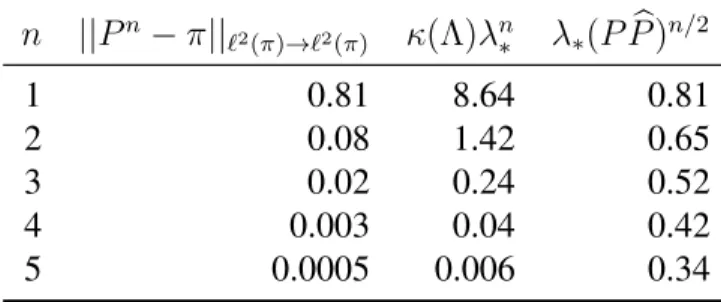
2.1 `2_{(π)-rate of convergence of}_P _{. . . .} ₆₀

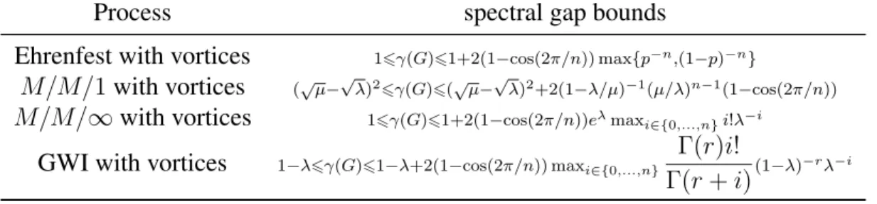
4.1 Spectral gap bounds for various birth-death processes with n-dimensional cyclic vortices . . . 124

(14)

CHAPTER 1

INTRODUCTION

Consider a Markov chain with transition kernelP and stationary distributionπ with its time-reversalP∗ on a general state space X. In the reversible case, that is, when P is viewed as a linear self-adjoint operator in the weighted Hilbert spaceL2_{(π), the}

quan-titative rate of convergence to equilibrium, as measured in the Hilbert space topology, total variation distance or separation distance, is well-known to be closely connected to the spectrum or the spectral gap ofP, see for instance Aldous and Fill [1], Levin et al. [74], Meyn and Tweedie [78], Miclo [81], Montenegro and Tetali [84], Saloff-Coste [97] and the references therein. Roberts and Rosenthal [93] shows that the existence of aL2

-spectral gap is equivalent toP being geometrically ergodic. The main technical insight relies heavily on the spectral theory of self-adjoint operators, which facilitates the anal-ysis of the spectrum ofP. From an application point of view, reversible Markov chains form the backbone in many diverse areas ranging from Markov chain Monte Carlo (see e.g. Roberts and Rosenthal [94] and Diaconis et al. [34]) or in the study of population genetics and community ecology (see e.g. Khare and Zhou [65] and Griffiths [46]). However,P need not be reversible in general. IfP is non-reversible, the analysis on the rate of convergence is fragmentally understood, possibly due to a much less developed spectral theory for non-self-adjoint operators. We refer interested readers to the work of Montenegro and Tetali [84], Wilmer [112] and Lorek [75] for excellent discussion on the convergence rate of some particular non-reversible Markov chains.

On the other hand, in addition to the theoretical interest as described above, the study of non-reversible Markov chains is also fascinating from an application perspective. It has been shown in Hwang et al. [53,54] and Chen and Hwang [18] that one can accel-erate the convergence of Markov processes by adding anti-symmetric drift to a common

(15)

underlying equilibrium. Diaconis et al. [33] proposes a non-reversible Markov chain sampler and analyzes the convergence rate in total variation distance, and more recently Sun et al. [106] and Bierkens [6] propose a non-reversible Metropolis-Hastings method by inserting vortices or perturbations to improve convergence rate, while Duncan et al. [35] studies non-reversible Langevin samplers and demonstrates a faster convergence rate with smaller asymptotic variance both theoretically and empirically. In this view-point, it is interesting to see if one can derive new algorithms to speed up convergence and offer an unifying framework for the analysis of non-reversible Markov chains.

We now give a historical account of the theoretical development and describe three different approaches that have been elaborated to deal with non-reversibility.

The first approach, suggested by Kendall [62], shows that non-reversible Markov kernel can be “dilated” to a semigroup of unitary operators in a larger Hilbert space by Sz.-Nagy’s dilation theorem. Yet, this approach seems to be dedicated enough to yield useful information on the rate of convergence. In this spirit of modifying the functional space, it is recently proposed by Kontoyiannis and Meyn [67] to castP in a weighted Banach space L∞_V instead of the classicalL2_(π)_{framework, where} _V _{is the}

Lyapunov function associated withP. In particular, they show that for a φ-irreducible and aperiodic Markov chain,P is geometrically ergodic if and only ifP admits a spectral gap in the spaceL∞_V equipped with theV-norm. They also give an example in which a non-reversible Markov chain is geometrically ergodic yet it fails to have aL2(π)spectral gap.

The second approach, initiated by Fill [42], is to resort to an appropriatereversiblized version of P and analyze how its spectrum can be related to the chi-squared distance to stationarity of the original chain. Two reversiblizations are proposed, namely the multiplicative reversiblization P P∗ and the additive reversiblization (P +P∗)/2. In

(16)

the discrete-time setting, it is shown that the second largest eigenvalue ofP P∗ can be used to upper bound the distance from stationarity, while the spectral gap of(P+P∗)/2 is used for continuous-time Markov chain. More recently, Paulin [89] generalizes this approach and defines apseudo-spectral gap, based upon the maximum spectral gap of P∗kPk fork _>1. He demonstrates that the proposed gap plays a similar role as that of spectral gap in the reversible case. He proves variance bounds and Bernstein inequality based on his proposed gap. In this fashion, we will explain an original approach that involves two types of Metropolis-Hastings reversibilizations in Chapter4.

The third approach, presented by Patie and Savov [85], is to resort to the concept of intertwining to build a link between non-reversible and reversible operators. More precisely, they investigate the rate of convergence to equilibrium of the so-called gener-alized Laguerre semigroups which are associated to non-self-adjoint integro-differential operators, and obtained explicit spectral estimate for the hypocoercivity phenomenon of this class. We will illustrate the spectral theory of skip-free Markov chains and more general non-reversible Markov chains via the concept of similarity, that is, an inter-twining relationship with the link operator having a bounded inverse, in Chapter2and Chapter3respectively.

1.1

Organization and outline of the Thesis

This thesis consists of four self-contained chapters, with a recurrent theme of analyzing non-reversible Markov chains from various perspectives. We now summarize the con-tributions and give a high-level discussion of the content in each chapter. Note that each chapter has its own introduction and a more detailed outline of the work.

(17)

Markov chains on denumerable state space. This encompasses their potential theory via an explicit characterization of their potential kernel expressed in terms of family of fundamental excessive functions, which are defined by means of the theory of Martin boundary. We also describe their fluctuation theory generalizing the celebrated fluctua-tions identities that were obtained by using the Wiener-Hopf factorization for the specific skip-free random walks. We proceed by resorting to the concept of similarity to identify the class of skip-free Markov chains whose transition operator has only real and simple eigenvalues. We manage to find a set of sufficient and easy-to-check conditions on the one-step transition probability for a Markov chain to belong to this class by stochas-tic monotonicity as introduced by Siegmund [102] and Clifford and Sudbury [22]. We also study several properties of this class including their spectral expansions given in terms of Riesz basis, derive a necessary and sufficient condition for this class to exhibit a separation cutoff, and give a tighter bound on its convergence rate to stationarity than existing results.

Chapter3. Building upon the work of Chapter2, we further examine the spectral the-ory of Markov chains on a denumerable state space from a similarity orbit perspective in this Chapter, expanding along the intertwining approach proposed by Patie and Savov [85] and Miclo [83]. In particular, we study the class of Markov chains that are in the similarity orbit of normal Markov chains such as birth-death chains or reversible Markov chains, which allows us to derive spectral expansions and offer a detailed anal-ysis on the convergence rate, separation cutoff (Chen and Saloff-Coste [13], Diaconis and Saloff-Coste [31], Mao et al. [76]) andL2_{-cutoff (Chen and Saloff-Coste [12], Chen}

et al. [15]) of this class of non-reversible Markov chains that is otherwise inaccessi-ble. We also look into the problem of estimating the integral functionals from discrete observations for this class, extending the work of Altmeyer and Chorowski [2] in this direction. Finally, as illustrations, we investigate three particular similarity orbits of

(18)

reversible Markov kernels, that we call the permutation, pure birth and random walk or-bit, and analyze various variants of classical birth-death processes, such as the Ehrenfest model, linear birth-death process, quadratic birth-death process and M/M/∞ model and their relationships with orthogonal polynomials in these orbits. Another highlight of this approach is that the Markov chain and all other chains in its orbits share the same eigentime identity as studied by Aldous and Fill [1], Cui and Mao [25], Miclo [82].

Chapter4. In this Chapter, along the reversiblization approach suggested by Fill [42] and Paulin [89], we study two types of Metropolis-Hastings (MH) reversiblizations for non-reversible Markov chains with transition kernel P. While the first MH kernel is the classical Metropolis chain of P as introduced by Hastings [48], Metropolis et al. [77] and Roberts and Rosenthal [94], we identify a new self-adjoint yet possibly non-Markovian operator that we call the second MH kernel to capture the opposite transition effect of the first kernel. We state a version of Weyl’s inequality for the spectral gap ofP and its additive reversiblization in the finite state space case, and illustrate the sharpness of the inequality by investigating in details the asymmetric simple random walk on the n-cycle and on discrete torus. We proceed by defining a pseudo-spectral gap, that we call the MH-spectral gap, based on the spectrum of the two MH kernels. We show that the existence of a MH-spectral gap implies thatP is geometrically ergodic, and by Weyl’s inequality the second MH kernel is a contraction operator wheneverP is lazy and ergodic in the finite state space case. We carry out some numerical examples that reveal that our MH-spectral gap is, for non-reversible chains, a better estimate than the existing bounds found in the literature. Variance bounds are also proved in terms of the proposed gap. Finally, we revisit the notion of metastability and the Cheeger inequality, and offer a variant of these celebrated inequalities by means of comparison of the Dirichlet form between the non-reversible chain and the two MH kernels.

(19)

Chapter5. In the final Chapter, motivated by the work of Hsu et al. [50], we consider the problem of estimating the log-Sobolev constant and the eigenspace of transition matrix via a single sample path from a reversible and ergodic Markov chain, in order to yield a tighter mixing time estimate by the log-Sobolev upper bound (see e.g. Diaconis and Saloff-Coste [30]) and the Wilson’s method for the lower bound (see e.g. Saloff-Coste [98]). We rely on the well-known relationship between the spectral gap and the log-Sobolev constant to provide an interval estimator of the latter, and we invoke a variant of Davis-Kahansinθtheorem to prove statistical guarantee for our proposed estimator of the eigenspace. We then proceed to illustrate that the same idea can be used to estimate other functional constants such as the modified log-Sobolev constant and the Cheeger constant of the Markov chain.

(20)

CHAPTER 2

SKIP-FREE MARKOV CHAINS

2.1

Introduction

Let X = (Xn)n∈N be a Markov chain on the countable state spaceE = [[l,r]] ⊆ Z, where we use the notation [[ (resp. ]]) to denote that l (resp. r) may or may not be in E, defined on the filtered probability space (Ω,(Fn)n∈N,P = (P)x∈E). We denote its transition matrix by P = (p(x, y))x,y∈E. We assume further thatX is irreducible, i.e. for all x, y ∈ E˙ =]l,r[, p(n)_{(x, y) =}

Px(Xn = y) > 0 for some n ∈ N, and upward skip-free, i.e. for all x ∈ E, p(x, x+ 1) > 0 and p(x, x+y) = 0, y _> 2. We denote by SF be the set of such upward skip-free Markov chains (or transition operators) onE.

The aim of this Chapter to develop a comprehensive theory for the setSF, includ-ingthe potential theory, the fluctuation theoryand, resorting to the algebraic concept of similarity,the spectral theory. As a by-product, we also provide, for ergodic chains, a detailed analysis of the speed of convergence to stationarity and investigate the separa-tion cutoff phenomena.

We recall that under the additional condition thatp(x, x−y) = 0, y _>2, that is, it is also skip-free to the left,X ∈ SF becomes a birth-death chain. These chains have been and are still the object of intensive and fascinating studies. This probably originates from the seminal work of Karlin and McGregor [59], see also Lederman and Reuter [69], on the diagonalization of their transition operator that provide deep insights into fine distributional properties of these chains. Note that the spectral analysis of these operators has also revealed fascinating links with the theory of orthogonal polynomials

(21)

and Stieljes moment problem. A review of birth-death chains including their potential theory, is given below in Section2.2.2.

Our contributions to the theory of the classSF can be summarized as follows.

(i) Potential theory: We shall start our program by studying the potential theory of chains inSF. More specifically, we implement an original approach based on the theory of Martin boundary for Markov chains as developed by Dynkin [39] to ex-press their q-potential kernel. In this vein, we recall that in the specific case of birth-death chains, this q-potential is given in terms of the two fundamental so-lutions (the decreasing and increasing one) of a three-term recurrence equations (discrete analogue of a second order differential equation), see Section 2.2.2 for more details regarding this expression. In our context, the situation is more del-icate as one has to solve an infinite recurrence equation whose set of solutions does not seem to have been clearly identified in the literature. Although the issue of solving this equation is of algebraic nature, we shall elaborate a strategy based mostly on a combination of techniques from probability theory and potential the-ory. More specifically, instead of trying to identify directly the convex cone of q-excessive functions for the chain X ∈ SF, we take an alternative route which consists in characterizing theq-potential kernel in terms of the so-called fundamen-tal q-excessive (for short FqE) functions of three different chains: (X,_P), (X,Pb)

the dual chain as defined in (2.2.2) below and(X,_Py]), y ∈ E, where(X,_Py])is the Markov chain (X,_P)killed upon entering the half-line[[l, y], which is plainly an upward skip-free Markov chain on the state spaceEy]_{= (y,}_r_]].

(ii) Fluctuation identities: From this representation of theq-potential kernel, we derive the main fluctuations identities for chains in SF. We recall that the fluctuation theory, which is concerned with the distribution of the first visit of the chain to

(22)

some (finite or infinite) intervals is of great importance in many applications such as biology, epidemiology and also in ruin theory where the upward skip-free property is required. This theory is well established for the case of birth-death chains (skip-free on both sides), see e.g. Karlin and McGregor [58], Keilson [60]. On the other hand the famous Wiener-Hopf factorization technique has proven to be useful to characterize the law of the first exit times for the class of random walks, that is for Markov chains with stationary and independent increments, see Spitzer [104] for further details on these identities. We also mention the interesting work of Fill [43] where he characterizes the upward hitting time distribution of upward skip-free chain via establishing an intertwining with pure-birth chain. Our original approach goes decisively beyond these frameworks as it allows to treat in an unified way, not only the first upward passage time, but also the first downward passage time, including the possibility of undershoot, of the irreducible skip-free Markov chain. To implement our methodology on some specific examples, one merely needs to have access to a transformation (Laplace transform, Fourier transform, moment generating function. . . ) that determines the one-step transition kernel of the chain. We shall illustrate this idea by recovering, in a simple manner, Spitzer’s identities for skip-free random walks, and, by studying the first passage times of branching Galton-Watson processes with immigration, whose details will be provided in a subsequent paper [20]. We also mention that the continuous analogue of these results for skip-free continuous-time Markov processes on the real line has been detailed in [87] and applications to generalized Ornstein-Uhlenbeck processes and continuous branching processes with immigration are carried out in [72] and [86] respectively.

(iii) Spectral theory and its applications: We also aim at providing some insights into the spectral theory of the (transition operator of) Markov chains that belong to the

(23)

class SF. This is a challenging issue as the transition operator P of such a chain is non-self-adjoint (non-reversible) in the weighted Hilbert space `2_(π), _where _π

is the reference measure, implying that there is no spectral theorem available for such bounded linear operator. To overcome this difficulty, we propose an original approach based on the concept of similarity. More specifically, we introduce a subclass ofSF, denoted bySsf, whose each element is related to a (diagonalizable) transition matrix of a birth-death Markov chain via a certain commutation relation. Using this identity, we resort to some techniques from non-harmonic analysis to investigate how to transfer the known spectral information of the reversible birth-death transition operator to the non-reversible one in order to obtain its spectral decomposition. By means of the inverse spectral theorem we manage to show that the classSsf characterizes completely the family of transition operators inSF that have real and distinct eigenvalues. On the other hand, we shall provide a set of sufficient and easy-to-check conditions on the one-step transition probability for a Markov chain to belong to Ssf. It is worth mentioning that, to the best of our knowledge, this is the first identification of a class of non-reversible chains with such a spectrum. This is a useful fact which answers an open question raised by Fill [43] on understanding the class of skip-free chains that have real and non-negative eigenvalues.

We believe that this new way of classifying Markov chains based on similarity orbit is powerful enough to tackle many substantial and delicate problems arising in the analysis of such chains. To illustrate this fact, we provide the spectral decomposi-tion of their non-symmetric transidecomposi-tion matrices, the law of their first passage times, including the case with possible overshoot. We also study for ergodic chains inSsf the speed of convergence to equilibrium in both the `2(π)-topology and the total variation distance. In this line of work, we indicate that Miclo [82] has recently

(24)

in-troduced a new notion known as Markov similarity and compares the mixing speed of Markov similar generators. As for the speed of convergence to equilibrium, there is a vast literature devoted to this important topic in various settings. For instance, in the case when P is a linear self-adjoint operator in`2_(π)_{(reversible), the chain}

satisfies the spectral gap, which according to Roberts and Rosenthal [93], is equiv-alent to P being geometrically ergodic. In the non-reversible case, to overcome the lack of a spectral theory, many interesting reversibilization techniques have been implemented to obtain a quantitative rate of convergence and we refer the interested readers to Fill [42] and Saloff-Coste [97]. We propose an alternative ap-proach based on the concept of similarity which seems to be a natural extension of the spectral gap estimate developed in the reversible case. Moreover, our technique enables us to provide an explicit and a spectral interpretation as a perturbed spec-tral gap estimate of the (discrete) hypocoercivity phenomena that was introduced by Villani [109] for general non-self-adjoint semigroups. We also manage to obtain generalization to the class SM

sf, a subclass of Ssf with stochastic monotone time-reversal to be formally introduced in Section 2.6, of the remarkable spectral gap times mixing time going to infinityseparation cutoff criteria established by Diaconis and Saloff-Coste [31] for reversible birth-death chains, and recently by Mao et al. [76] for continuous-time skip-free chain with stochastic monotone time-reversal.

We point out that these three topics (potential, fluctuation and spectral theory) are intertwined. Indeed, there is of course a fundamental connection between the resolvent operator and the spectral theory of P as the spectrum of P is, by definition, the set of complex numbers z such that the resolvent operator Rz = (zI − P)−1 does not exist or is unbounded. Note that since P is a contraction operator, this set is included in the unit disc. Moreover, the development of the fluctuation identities is based on the expression of the q-potential kernels whereas the spectral theory allow us to get

(25)

an explicit representation of the transition kernel (and hence by integration of the q-resolvent operator) and, also, of the distribution of the first passage times.

The rest of the Chapter is organized as follows. In Section2.2, we fix our notations and provide a review of birth-death chains and Martin boundary theory. The definition and study of the fundamentalq-excessive functions as well as the expression of the q-potential kernel are discussed in Section2.3. In Section2.4, we present the fluctuations identities, that is the explicit characterization (via the probability generating function) of the law of the first exit times of skip-free chains, and, following the line of work by Feller [41], Kent and Longford [63] and Viskov [110], a characterization of these stopping times as discrete infinitely divisible variables in Section 2.5. We proceed in the Sections 2.6-2.8 by introducing the subclass of skip-free Markov chains that are similar to a diagonalizable birth-death chain and discuss their spectral properties as well as its applications to the speed of convergence to equilibrium and the study of the cutoff phenomena.

2.2

Preliminaries

In this Section, we review some classical concepts on Markov chains that will play a central role throughout the chapter. This include some facts of the potential theory and the Martin boundary theory of Markov chains.

2.2.1

Basic facts on Markov chains

We recall thatX is said to be upward skip-freeif the only upward transition is of unit size, yet it can have downward jump of any arbitrary magnitude, i.e. for allx ∈ E and

(26)

y _> x+ 2, _Px(X1 = y) = 0. We consider an upward skip-free irreducible Markov

chainX = (Xn)n∈_N0 on a denumerable state spaceE ⊆Zwith left endpointland right

endpointr. We use the convention thatr ∈ E if the boundary pointris not absorbing. Otherwise, if ris absorbing or r = ∞, we say that X ∈ SF∞. We assume now that

X ∈ SF∞and postpone to Section2.3.3the study of the Markov chainX /∈ SF∞.

SinceXis irreducible, there existsπa positive and finite-valued excessive measure forP, that is,πP ₆π, see [61, Section5.2and6.8], and that will serve as a reference measure. LetGq be the q-potential kernel ofX (or its Green function) with respect to the reference measureπ. That is, for0< q <1,

Gq(x, y) = ∞ X n=0 qnPx(Xn =y) π(y) = ∞ X n=0 qnp (n)_{(x, y)} π(y) , x, y ∈E. (2.2.1) Whenq = 1, we writeG, rather thanG1, to denote the 1-potential kernel. Theπ-dual

matrixPb = (p(y, x))y,x_b ∈E is defined to be

b

p(y, x)π(y) = p(x, y)π(x). (2.2.2) Denoteζ to be the lifetime ofX, that is,ζ(ω) = k ifkis the last time thatX is in the state spaceE, andζ(ω) = ∞otherwise.

Let us now define the hitting times associated with X. Denote TA to be the first hitting time of the set A, that is,

TA= inf{n_>0;Xn ∈A},

with the usual convention thatinf{∅} =∞. IfA ={a}, we writeTa = TA. Similarly, ifA= (l, b], we useTb] =TA. Denote the first return time to beTa+ = inf{n >1;Xn = a}.

(27)

notation, for anyx, y ∈E, P f(x) =X y∈E p(x, y)f(y), µP(y) =X x∈E µ(x)p(x, y).

2.2.2

A review of birth-death chains

LetY be a birth-death chain onEwith transition operatorQ∈ B, that is,Q∈ SF with the additional requirements thatQ(x, x−1) >0andQ(x, x−y) = 0fory _> 2. Qis a bounded self-adjoint operator in the Hilbert space`2(πQ) whereπQ is the reversible measure, i.e. for all x, y ∈ E, Q(x, y)πQ(x) = Q(y, x)πQ(y). The q-potential of Q, denoted byUq, is well-known to take the form, for anyx, y ∈E,

Uq(x, y) =CqFq(x∧y)Fb_q(x∨y), (2.2.3)

whereFq (resp. Fbq) is the unique increasing (resp. decreasing) solution to the equation

qQF =F satisfying appropriate boundary conditions, andCqis their Wronskrian. Note that this equation boils down to a three-term recurrence equations, see [38, Ex. 5.3 p.150 and Section 5.4] for details regarding this expression. This is reminiscent to the expres-sion of the potential kernel of the continuous time-space analogue, whose generator is a second order differential operator. We recall that a systematic and thorough study of one-dimensional diffusion has been undertaken by Feller [40]. Moreover, the moment generating function of the first hitting timeTY

a = inf{n > 0; Yn = a}ofY to a fixed levela ∈Eis given by Ex[qT Y a _{] =} Fq(x) Fq(a)1 {x6a}+ b Fq(x) b Fq(a) 1{x>a}. (2.2.4)

Let us now describe a link between this expression and the diagonalization of the op-eratorQ in B. We assume, for sake of simplicity, that l = 0 and thusE is countable

(28)

subset ofN. It is worth mentioning that the similarity transformD√πQD_√1

π, whereDa is the diagonal matrix ofayields to a symmetric tridiagonal matrix which belongs to the well-studied class of Jacobi matrices. We also recall that a functionφis a Pick function if φ admits an analytical continuation to the cut complex plane _C \[0,∞) such that =φ(z)=(z) _> 0, and we denote byP the subset of such Pick functions that admit the representation, for=(z)>0, φ(z) = Z 1 −1 d∆(r) r−z , (2.2.5)

where∆is a probability measure on [−1,1]. From the work of Karlin and McGregor [59], we know that there exists the spectral mappingK : B → P which is one-to-one and∆is the spectral measure ofQ. More specifically, we have for anyf ∈`2_(π

Q)and n∈_N,Qncan be diagonalizable as follows

Qnf =

Z 1

−1

rnhf,Friπ_QFrd∆(r), (2.2.6) where for r ∈ supp(∆), QFr = rFr. Note that S(Q) the spectrum of Qis such that S(Q) = supp(∆) ⊂ [−||Q||,||Q||] ⊆ [−1,1]. Another remarkable and deep result, which is due to Krein, is the onto property of the spectral mapK. Indeed for anyφ ∈ P, i.e. a Pick function of the form (2.2.5), there exists an unique Q ∈ B on E with l a non-killing boundary with a spectral representation of the form (2.2.6). The first proof of this conjecture was given in [38, Chapter 6]; it uses the theory of Hilbert spaces of entire functions, and a deep uniqueness theorem due to de Branges. Note also that such a spectral representation reveals that when the spectrum ofQ is composed of isolated eigenvalues then they are necessarily simple (see e.g. Karlin and McGregor [59] and [38]).

(29)

2.2.3

Martin boundary theory of denumerable Markov chains

In this subsection, we review some essential results of Martin boundary theory of de-numerable Markov chains based on [39, 61, 113]. First, we recall the definition of q-excessive, q-harmonic andq-potential functions. A non-negative functionf on E is q-excessive (resp.q-harmonic) ifqP f(x)₆f(x) (resp. qP f(x) =f(x))for allx∈E, where0 < q ₆ 1. A non-negative functionf onE is a q-potential if f isq-excessive andlimn→∞(qP)nf(x) = 0for allx∈ E. We say thatf is harmonic (resp. excessive)

iff is1-harmonic (resp.1-excessive). Note that the irreducibility property implies that f ∈ Eq is positive, since if there existsy∈ Esuch that f(y)>0, then by irreducibility there existsnsuch that forx∈E f(x)_>qpn_{(x, y)f}_(y)_>_{0. We write}

Eq ={f :E →R+; qP f 6f}(resp.Hq,Pq)

to be the set ofq-excessive (resp. q-harmonic, q-potential) functions onE. We simply writeE (resp.H,P) to denote the set of excessive (resp. harmonic, potential) functions. We will also use the notationEbq(resp.Hbq,Pbq) to denote the set ofq-excessive (resp.

q-harmonic, q-potential) functions associated with Pb, which was defined in (2.2.2). We

point out that if ˆh ∈ Eb_q, then ˆhπ is a q-excessive measure for P in the sense that

qˆhπP f ₆ ˆhπf. Another commonly used terminology for excessive (resp. harmonic, potential) function is superharmonic (resp. invariant, purely-excessive) function.

We further recall the definition of minimalq-harmonic function. A non-zero function f on E is minimal q-excessive if f = f1 +f2 implies f = cifi for i = 1,2, where

f1, f2 ∈ Eq,c1 andc2are constants and0 < q 61. We say thatf is minimal excessive

if f is minimal 1-excessive. We write Emin

q (resp. Hminq ) to be the set of minimal q-excessive (resp. minimalq-harmonic) functions onE. Next, we state the classical Riesz representation theorem, which gives an unique decomposition of excessive function.

(30)

Theorem 2.2.1(Riesz representation theorem). For0< q ₆1, everyq-excessive func-tion can be written uniquely as the sum of aq-potential and aq-harmonic function. That is, iff ∈ Eq, then

f(x) =X y∈E

Gq(x, y)kq(y)π(y) +hq(x),

wherekq(x) = f(x)−qP f(x)andhq(x) = limn→∞(qP)nf(x)∈ Hq.

Suppose(X,_P)is a transient Markov chain with transition matrixP and reference measureπon a denumerable state spaceE. For a measureµonE, defineEµ = {y ∈ E; µG(y) > 0}, where µG(y) = P

x∈Eµ(x)G(x, y). We say that the measure µis a standard measure if Eµ = E. For x, y ∈ E and 0 < q ₆ 1, the q-Martin kernel associated to a standard measureµis defined to be

µKq(x, y) =

Gq(x, y) µGq(y)

, (2.2.7)

where the denominator is positive sinceµis standard. SinceXis transient,µKq(x, y)is finite for anyx, y ∈E. Next, define a metricµdqon the spaceE by

µdq(y, z) = X x∈E wx |µKq(x, y)−µKq(x, z)|+|1{x=y}−1{x=z}| Cxµ+ 1 , where the weights(wx)x∈E, withwx >0, are chosen such that

P

x∈Ewx <∞, andCxµ is a function that depends only onxand satisfies µKq(x, y) ₆ C_xµ. We can obtain the completion ofE with respect to the metricµdq, namelyE, and the boundary ofE inE is denoted as∂E =E−E. Eis the Martin compactification ofE and∂Eis the Martin boundary. The set

∂_PE ={y∈∂E; µKq(x, y)is minimalq-harmonic inx}

is known as theminimal Martin boundary. When there is no ambiguity in the probability measure, we write∂mE =∂PE. The inclusion of the indicator terms1{x=y}and1{x=z}

(31)

Martin boundary∂E is closed. Next, fix a reference pointo< r−1, and we write the q-Martin kernelδoKq(x, y)as δoKq(x, y) = µGq(y) Gq(o, y) µKq(x, y) = µKq(x, y) µKq(o, y) . Similarly, we have µKq(x, y) = Gq(o, y) µGq(y) δoKq(x, y) = δoKq(x, y) µKq(y) .

A sequence (yn) is a Cauchy sequence in the metric space (E,µdq) if and only if (µKq(x, yn)) is a Cauchy sequence of real numbers for every x if and only if (δoKq(x, yn)) is a Cauchy sequence of real numbers for every x if and only if (yn)is

a Cauchy sequence in the metric space (E,δodq). Thus, up to homeomorphism, E is

independent of the choice of the reference pointo. It can also be shown thatE is inde-pendent of the choice of the weights(wx)x∈E (see e.g. Proposition 10.13 in [61]). From now on, we fix the reference pointoand write

Kq(x, y) = δoKq(x, y) =

Gq(x, y) Gq(o, y).

LetΩ∞ = {ω; there isx∞ ∈ ∂Esuch thatxn → x∞in the Martin topology}.Ω∞can

be interpreted as the set ofnon-terminatingtrajectories of X that converges to ∂E. If (X, P) is transient and P is a stochastic matrix then there is a random variable X∞

taking values in∂E such that for eachx ∈E,_Px(limn→∞Xn =X∞) = 1.In terms of

trajectory space, we have_Px(Ω∞) = 1.IfP is strictly substochastic at some states, we

should extend the trajectories toE∪ {∇}, where∇is the graveyard state. Define Ω∇={ω; there isk>1such thatxn ∈E, ∀n 6kandxn =∇,∀n >k+ 1}. Ω∇ is the set of trajectories that eventually reach∇. Denoteζ to be the lifetime of X,

that is, ζ(ω) = K for ω ∈ Ω∇, where K is the last time thatX is in the state space

(32)

transient then there is a random variableXζtaking values inEsuch that for eachx∈E,

Px(limn→ζXn=Xζ) = 1.In terms of trajectory space, this means thatPx(Ωζ) = 1. Next, suppose now that h ∈ Eq. The h-process ofX is defined to be the Markov chain onEh ={y ∈E; h(y) >0}=E, by irreducibility, with the canonical measure

Phx such thatPhx(X1 = y) =

p(x, y)h(y)

h(x) .Recalling that ois the fixed reference point, theq-potential andq-Martin kernels associated with theh-process take respectively the form

Gh_q(x, y) = Gq(x, y)h(y)

h(x) , (2.2.8)

K_qh(x, y) = Kq(x, y)h(o)

h(x) . (2.2.9)

From (2.2.9) and the definition of the metricµdq, we observe that the Martin compacti-ficationE is homeomorphic to the Martin compactification of theh-process. Next, we state the following which are the main claims of Theorem6and7in [39].

Theorem 2.2.2(Uniqueness of the representation). Letq ∈ (0,1]. Ifh ∈ Eq such that h(o) = 1thenhhas a unique representation of the form

h(x) =

Z

E∪∂mE

Kq(x, y)µh(dy) = Kqµh(x),

where µh(·) = Ph(Xζ ∈ ·) defines a probability measure. Conversely, for any finite measure µ, the mapping x 7→ R

E∪∂mEKq(x, y)dµ(y)defines an q-excessive function, which isq-harmonic if and only ifµ(E) = 0. Finally, for ally∈ E∪∂mE, lethy(·) = K(·, y). Then y ∈ E ∪∂mE if and only if Ph

y

(Xζ = y) = 1. Moreover we have

Ph

y

(ζ =∞) = 1if and only ify ∈∂mE.

The previous claim means that X is forced to terminate at the pointy ∈ E∪∂mE

Ph

y

x -almost surely.

Theorem 2.2.3. We haveEmin

(33)

Finally, we recall the following useful result whose proof follows readily from [21, Theorem11.9].

Lemma 2.2.1. Suppose thathq ∈ Eq, andT is a stopping time with respect to(Fn)n>1.

Forx∈Ehq, Phqx (T <∞) = 1 hq(x)E x qThq(XT)1{T <∞} .

2.3

Potential Theory

In this Section, we provide an explicit representation of the q-potential kernelGq, as defined in (2.2.1), of an upward skip-free Markov chainX ∈ SF. We recall that in the simpler case when X boils down to a birth-death Markov chain, i.e. skip-free in both directions, then itsq-potential kernel takes the form

Uq(x, y) =CqFq(x∧y)Fb_q(x∨y), (2.3.1)

where Fq and Fb_q are the two fundamental solutions of a three-term recurrence

equa-tions (discrete analogue of a second order differential equation), see Section 2.2.2for more details regarding this expression. In our context, the situation is more delicate as one has to solve an infinite recurrence equation whose set of solutions does not seem to have been clearly identified in the literature. Although the issue of solving this equation is of algebraic nature, we shall elaborate a strategy based mostly on a combination of techniques from probability theory and potential theory. We start by expressing the q-potential kernel in terms of the so-called fundamentalq-excessive (for short FqE) func-tions of the following three processes: (X,_P), (X,bP)and (X,Py]), where (X,Py])is

the Markov chain (X,_P) killed upon entering the half-line [[l, y], which is plainly an upward skip-free Markov chain on the state spaceEy] _{= (y,}_r_{]], with transition kernel}

(34)

Theorem 2.3.1. 1. Writing, for anyx∈Eand0< q <1,

Hq(x) = Kqδr(x), (2.3.2) (resp.Hb_q(x) = Kb_qδ_l(x)) withδ_ris the Dirac mass atr, we have, for all0< q <1,

that

Hq ∈ E_qmin

(resp.Hb_q ∈ Eb_qmin) and it is the unique minimal increasing (resp. decreasing)

q-excessive forP (resp.Pb) such thatH_q(o) = 1(resp. Hb_q(o) = 1). Moreover, if

X ∈ SF∞(resp.X ∈ SF \ SF∞) thenHq is the unique increasing function in Hq(resp.Hq ∈ PqwithHq(r)<∞).

2. For any y < r, 0 < κyq] = lim x→r

Kqδr(x)

Kqy]δr(x)

< ∞. Then the functionHyq]defined, for anyx∈Ey]_{, by}

Hy_q](x) =κ_qy]K_qy]δr(x) (2.3.3) has (with respect toPy]_{) the same property than}_H

qbut with the normalization

lim x→r

Hyq](x) Hq(x) = 1 (recall that by conventionHyq](x) = 0for anyx6y).

3. Finally, let X ∈ SF∞ and set Cq = Gq(o,o) > 0. Then, we have, for all x, y ∈E,

Gq(x, y) =CqHb_q(y) H_q(x)−Hy_q](x)

. (2.3.4)

Remark2.3.1. Up to minor modifications all statements hold forq = 1when(X,_P)is transient.

Remark2.3.2. The terminology FqE comes from the birth-death case where these func-tions are usually called the fundamental solufunc-tions of the associated three-term recurrence equation and areq-excessive.

(35)

Remark2.3.3. In comparison to the expression of theq-potential of the birth-death chain given in (2.3.1), there is in addition to the (unique) FqE functions for(X,_P)and its dual (X,bP), the sequence of FqE functions associated to the family of killed Markov chains

(X,_Py]₎

y∈E.

Remark2.3.4. Additional properties of Hq and its relation with infinite divisibility are studied in Section2.5Corollary2.5.1.

We proceed with the proof of these statements which is split into several intermediate results.

2.3.1

Proof of Theorem

2.3.1

We start with the following result which relates the Martin kernel to the hitting time distribution.

Lemma 2.3.1. For anyx, y ∈E,

Ex(qTy) =

Kqδy(x) Kqδy(y) .

Proof. By Theorem2.2.1, for anyy ∈ E, Kqδy ∈ Pqwhich leads, by Theorem2.2.2, to_PKqδy(Xζ =y, ζ <∞) = 1, that is, for anyx, y ∈E,

PKqδyx (Ty <+∞) = 1.

Since, on the other hand, by Lemma2.2.1, we have, for anyx, y ∈E,

PKqδyx (Ty <+∞) =Ex(qTy)

Kqδy(y) Kqδy(x) we complete the proof.

(36)

Proof of Theorem2.3.1(1)

Suppose thatx∨o₆y₆a, wherex∨o= max{x,o}. By means of Lemma2.3.1, the upward skip-free property and the strong Markov property, we obtain that

Kqδa(x) = Ex(q Ta₎ Eo(qTa) = Ex(q Ty₎ Ey(qTa) Eo(qTy)Ey(qTa) =Kqδy(x). (2.3.5) Thus, for anyy _> x∨o, Kqδy(x) = Kq(x, x∨o). Hence, one can trivially define the functionHqas the extended Martin kernel atr, that is, forx∈E,

Hq(x) = lim

y→rKq(x, y) =

Z

E∪∂mE

Kq(x, y)δr(dy).

Hence if X ∈ SF∞ (resp. X ∈ SF \ SF∞) then r ∈ ∂_PE (resp. r ∈ E) and thus

by theorems2.2.2and 2.2.3(resp. and Theorem2.2.1), we get thatHq ∈ Hq ∩ Eqmin (resp. Hq ∈ Pq∩ Eqmin). Next note, from the first identity in (2.3.5), thatHq(o) = 1, and, forx₆y,Hq(x) = Kqδy(x). Hence, by Lemma2.3.1we have, for anyx6y,

Ex(qTy) =

Hq(x)

Hq(y), (2.3.6)

which entails, by the irreducibility of X, that Hq is positive everywhere since for any x∈E, the ratioHq(x) = Ex(qTa)

Eo(qTa) >0. To see that the mappingx7→Hq(x)is increasing,

one observes from again the strong Markov property and the upward skip-free property that (recall thatx₆y₆a)

Hq(x) = E

x(qTy)Ey(qTa)

Eo(qTa)

=_Ex(qTy)Hq(y)< Hq(y).

To prove the uniqueness, we proceed by contradiction and thus assume that there exists a positive function hq ∈ Eqmin (resp. in Hq when X ∈ SF∞) which differs from Hq and which is also an increasing function onE. Then, according to Theorem2.2.3, there existsy0 ∈ E (resp.y0 =lory0 =r) such that for allx ∈ E, hq(x) =

Kq(x,y0)

Kq(o,y0). Thus,

on the one hand, from Lemma2.3.1we deduce that for anyx₆y0, Ex(qTy) = Kqδy0(x) Kqδy0(y0) = hq(x) hq(y0) .

(37)

This combines with (2.3.6) yield thathq(x) =Hq(x)for anyx 6y0, which proves the

claim whenHq ∈ Hq andy0 = r. In the other cases, choosex > y0 such thathq(x) 6= Hq(x). Then, observe from Theorem 2.2.2that P

hq

x (Ty0 < +∞) = 1. As P hq

x (Ty0 < +∞) = hq_hq(₍y0_x₎)_Ex(qTy0)andhqis increasing andx > y0, we get thatEx(qTy0)>1which is impossible. This completes the uniqueness property of Hq. To complete the proof of Theorem2.3.1(1), we use similar arguments for deriving the stated properties ofHqb

after recalling that the dual chain(X,bP)is downward skip-free.

Proof of Theorem2.3.1(2)

We start with the following claim which is a straightforward reformulation of Theorem 2.3.1(1) for the killed chains.

Lemma 2.3.2. Letb ∈E and choose a reference pointob] _∈_Eb]_{. Then, for all}₀_{< q <}

1, the functionHqb](x) =Kqb]δr(x)defined onEb]is positive onEb], minimal, increasing q-harmonic forPb]withHqb](ob]) = 1. Moreover, for anyb6x6a,

Ebx](q Ta ) = _Ex(qTa₁{Ta<Tb]}) = Hqb](x) Hqb](a) .

Proof. Under_Pb], X is an upward skip-free Markov chain onEb], the results follows from Theorem2.3.1(1) and the identity (2.3.6).

The following lemma expresses the pgf of the downward hitting times (Tb,P

[a x), wherea > x > b, in terms of the FqE functions of(X,_P)and(X,_Pb]).

Lemma 2.3.3. For anyb < x < aand0< q <1, we have

Ex(qTb1{Tb<Ta}) = Hq(x) Hq(b) − Hq(a) Hq(b) Hqb](x) Hqb](a) .

(38)

Proof. Since by definitionHq =Kqδr, we have, from Theorem2.2.2that,

PHq(Xζ =r) = 1. (2.3.7)

This combines with the upward skip-free property, see Lemma2.2.1, yields that under

PHqx the sample paths of X that drop below b before hitting a must reaches b before reachinga. That is

PHqx (Tb < Ta) = PHqx (Tb]< Ta) = 1−PHqx (Ta< Tb]), (2.3.8)

where we used again (2.3.7) for the second identity. Hence, an application of Lemma 2.2.1gives PHqx (Tb < Ta) = Hq(b) Hq(x)E x(qTb1{Tb<Ta}) = 1− Hq(a) Hq(x)E x(qTa1{Ta<Tb]}) = 1− Hq(a) Hq(x) Hqb](x) Hqb](a) , where the last equality follows from Lemma2.3.2. Rearranging the terms provides the desired result.

The proof of Theorem2.3.1(2) follows readily after the following claim.

Lemma 2.3.4. Forx∈Eb], define

κb_q](x) = Hq(x) Hqb](x) .

Then the mappingx7→κbq](x)is non-increasing onEb]with0< κbq](x)<∞. Further-more,0< κbq]= limx→rκ

b]

q(x)<∞.

Proof. It is clear that, for all x ∈ Eb], 0 < κqb](x) < ∞, since both Hq and H b]

q are positive and finite onEb]. Next, for anyx∈Eb],

(39)

where the first inequality follows from the fact that Pb] _{is the restriction of}_P _to _Eb]_,

and we use thatHq ∈ Eq in the second inequality. Therefore,Hq (restricted onEb]) is q-excessive forPb]_{. Thus, one may define the}_H

q-transform ofqPb]by Hq_Pb]_{(x, y) =} Hq(y)

Hq(x)

qPb](x, y),

wherex, y ∈ {x∈Eb]: Hq(x)>0}=Eb]by Theorem2.3.1. Using Lemma2.2.1and Lemma2.3.2, we have, for anyx₆a,

Hq Pbx](Ta <∞) = Hq(a) Hq(x)E b] x(q Ta_{) =} H b] q(x) Hq(x) Hq(a) Hqb](a) = κ b] q(a) κbq](x) . (2.3.9) Since (X,Hq

Pbx]) is a transient upward skip-free Markov chain, using Lemma 2.3.1 and Theorem 2.3.1(1) for q = 1, one easily deduces, with the obvious notation, that

1

Cκb]q(x)

= Hq_Kb]_δ

r(x), for some C > 0. Thus the mapping x 7→ κ b]

q(x) is non-increasing. Henceforth κbq] = limx→rκ

b]

q(x) 6 κbq](b+ 1) < ∞. Observing that both Hq(r)andH

b]

q(r)are finite when X ∈ SF \ SF∞, we readily get that κbq] > 0which completes the proof in this case. It remains to show that

lim a→r κbq](a) κbq](x) = lim a→r Hq Pbx](Ta <∞)>0, (2.3.10) whenX ∈ SF∞. To this end, we assume the contrary, that is,lima→rHqP

b]

x(Ta<∞) = 0. SinceHq_Pbx](Ta < ∞) =P

Hq

x (Ta < Tb]), the assumption becomeslima→rP Hq x (Ta < Tb]) = 0and (2.3.8) leads to lim a→rP Hq x (Ta< Tb) = 0. (2.3.11) Next, by means of a first step analysis and the upward skip-free property, we obtain

PHqb (T + b < Ta) =pHq(b, b+ 1)P Hq b+1(T + b < Ta) +pHq(b, b) + X y<b pHq(b, y)_PHq_y (T_b+ < Ta). (2.3.12)

(40)

Takinga→r, the left-hand side converges toPHqb (T

+

b <∞)(recall thatT

+

b = inf{n> 1; Xn = b}) due to the monotone convergence theorem, the upward skip-free prop-erty and the fact that X ∈ SF∞. On the right-hand side of (2.3.12), the first term

converges to pHq_{(b, b} _{+ 1)} _{as a result of (2.3.11), while the third term converges to}

P

y<bp

Hq_{(b, y)}

PHqy (T_b+<∞)by invoking the dominated convergence theorem. There-fore, we arrive at PHqb (T + b <∞) = p Hq_{(b, b}_{+ 1) +}_pHq_{(b, b) +}X y<b pHq(b, y)_PHq_y (T_b+<∞) =pHq(b, b+ 1) +X y6b pHq(b, y) =_PHq_b (ζ >1) = 1,

where the second equality comes from the identity PHqy (T_b+ < ∞) = 1 which holds since _PHqy (Xζ = r) = 1 and y < b, while the last equality is due to Theorem 2.2.2 with the fact thatHq ∈ Hq sinceX ∈ SF∞. This is not possible since X is transient.

Therefore, we conclude thatκbq]>0.

2.3.2

Proof of Theorem

2.3.1

(

3

)

We start with the following extension of Lemma2.3.3.

Lemma 2.3.5. For anyx, y ∈Eand0< q <1, we have

Ex qTy = Hq(x)−H y] q(x) Hq(y) . (2.3.13)

Proof. The case whenx ₆ yis proved in (2.3.6). Next assume thatx > y. Thanks to the upward skip-free property ofX, for anyb ∈Ethe mapping₁{Tb<Ta}is increasing in

alarge enough. Then, the monotone convergence theorem and the fact thatX ∈ SF∞

give lima→rEx(qTb1{Tb<Ta}) = Ex(qTb). The sought result follows immediately from Lemma2.3.3and Lemma2.3.4.

(41)

We are now ready to prove the expression (2.3.4). First using (2.3.6), Lemma2.3.1 and the definition of the Martin kernel in (2.2.7), we obtain, for anyx₆o,

Ex(qTo) = Hq(x) = Gq(x,o) Gq(o,o) = Gq(x,o) Cq . (2.3.14)

Next, for sake of clarity we state the analogue of the identity (2.3.6) for the dual chain (X,bP).

Lemma 2.3.6. For all0< q <1and anyx₆y,

b Ey(qTx) = b Hq(y) b Hq(x) . (2.3.15)

A specific application of the previous result yields, for anyx₆o, that

b Eo(qTx) = 1 b Hq(x) = Gq(b o, x) b Gq(x, x) = Gq(x,o) Gq(x, x) , (2.3.16)

where we use the identityHb_q(o) = 1 in the first equality, the dual version of (2.3.14)

for the second one and the integrated version of the dual identity (2.2.2) for the last one. Combining (2.3.14) and (2.3.16), we get, for anyx₆o,

Gq(x, x) = CqHq(x)Hb_q(x). (2.3.17)

For anyx_>o, we reverse the role ofxandoto obtain, respectively,

Eo(qTx) = 1 Hq(x) = Gq(o, x) Gq(x, x), (2.3.18) b Ex(qTo) = Hb_q(x) = b Gq(x,o) b Gq(o,o) = Gq(o, x) Gq(o,o). (2.3.19) Combining (2.3.18) and (2.3.19), we again arrive at (2.3.17), which shows that (2.3.17) holds for all x ∈ E. Note that (2.3.17) holds regardless of the boundary condition at

r. In particular, when X ∈ SF∞, (2.3.13), (2.3.14) (replacing y by o), (2.3.17) and

(42)

2.3.3

X

∈ SF \ SF

∞

We suppose, in this Section, thatX ∈ SF \ SF∞, that is, ris a regular boundary. The

state spaceEincludes the pointr, that is,E = [[l,r]. Under_P[r_,_X_{is a skip-free Markov} chain on the state spaceE[r _{= [[}_l_,_r_{), which is killed whenever the process hits the state}

r. We are ready to state the following.

Proposition 2.3.1. Supposeris a regular boundary. Then for anyx > b,

Ex(qTb) =          Hq(x)−K¯ b] qHqb](x) Hq(b) ifr> x > b, Gq(r, b) Gq(b, b) ifr=x > b, whereK¯qb]= G[qr(o,o)Hb [r q(b) Gq(o,o)Hb_q(b) andGq(r, b) = ηb(q) c+ (1−q)p+P j∈E(1−q)ηj(q) ,where c_>0,p > 0, andη(q) = (ηj(q))j∈E is a family of non-negative numbers that satisfies, for any0< s, q <1,

sη(s)−qη(q) = (s−q)η(q)G[_qr, whereG[qr= (G[qr(i, j))i,j∈E.

In order to prove this Proposition, we need the following classical result that enables to connect theq-potential ofGqandG

[a

q (resp. Gb_qandGb

b]

q).

Lemma 2.3.7. We have, for any0< q <1,

Gq(x, y) = G[_qa(x, y) +_Ex(qTa)Gq(a, y), x, y ∈E[a, (2.3.20)

b

Gq(x, y) = Gbb_q](x, y) +Eb_x(qTb)Gb_q(b, y), x, y ∈Eb]. (2.3.21)

(43)

we have Px(Xn =y) = P[xa(Xn =y) + n−1 X k=1 Px(Xn =y|Ta=k)Px(Ta =k) =_P[_xa(Xn =y) + n−1 X k=1 Pa(Xn−k =y)Px(Ta=k),

where the second equality follows from strong Markov property. Next, multiplying by qn_{, dividing by}_{π(y), which is positive by irreducibility, and summing over}_{n, we obtain}

Gq(x, y) = G[qa(x, y) + ∞ X n=1 n−1 X k=1 qn−kPa(Xn−k=y) π(y) q k Px(Ta=k) =G[_qa(x, y) + ∞ X k=1 ∞ X n=k+1 qn−kPa(Xn−k =y) π(y) q k Px(Ta=k) =G[_qa(x, y) +_Ex(qTa)Gq(a, y)

which proves (2.3.20). (2.3.21) is the dual statement of (2.3.20).

We are now ready to complete the proof of Proposition 2.3.1. First, observe that (X,_P[r₎_{∈ SF}

∞and thus by means of Lemma2.3.7and (2.3.17), one gets

Gq(b, b) = G[qr(o,o)H [r q(b)Hb_q[r(b) + Hq(b) Hq(r) Gq(r, b). (2.3.22) If one chooses the same reference pointofor(X,_P)and(X,_P[r_{), then plainly, for any} x∈E[r_,_H

q(x) =H

[r

q(x), this leads, using again (2.3.17), to Gq(o,o)Hb_q(b) = G_q[r(o,o)Hb_q[r(b) +

Gq(r, b) Hq(r)

. (2.3.23)

Forr> x > b, using the lemmas2.3.1and2.3.7, we have

Ex(qTb) = Gq(x, b) Gq(b, b) = G [r q(x, b) +Ex(qTr)Gq(r, b) Gq(o,o)Hq(b)Hbq(b) = G[qr(o,o)(Hq[r(x)−Kqb]Hqb](x))Hb [r q(b) + Hq_Hq(₍x_r₎)Gq(r, b) Gq(o,o)Hq(b)Hbq(b) = Gq(o,o)Hq(x)Hq(b)b −G [r q(o,o)Hqb](x)Hb [r q(b) Gq(o,o)Hq(b)Hb_q(b) = Hq(x)−K¯ b] qHqb](x) Hq(b) ,

(44)

where we used (2.3.23) in the fourth equality. Forx = r > b, it follows from (2.3.17) that Er(qTb) = Gq(r, b) Gq(b, b) = Gq(r, b) Gq(o,o)Hq(b)Hbq(b) .

To complete the proof one appeals to Theorem 3.1 of [92] that enable to determine Gq(r, b).

2.4

Fluctuation identities

We pursue our program by exploiting the potential theoretic results of the previous Sec-tion to derive the fluctuaSec-tion identities of a general skip-free Markov chain. This consists in determining the law, through the pgf, of the first exit time ofXto a (in)finite interval. These quantities are critical in many applications in various settings including insurance mathematics, biology and epidemiology to name but a few. For instance, the timeT0]

corresponds to the time of ruin for a risk process having only negative jumps, which is a natural assumption in risk theory as they (the jumps) model the size of claims. We emphasize that our methodology enables to get the pgf of this time of ruin and hence al-lows to solve this problem for general Markovian risk processes. We also recall that for a birth-death chain the pgf of exit times is given as a linear combination of the two FqE functions, the one for(X,_P)and its dual(X,Pb). There exists also a theoretical

charac-terization of the laws of these variables for random walks through the celebrated Wiener-Hopf factorization. This technique, which is of complex analytical nature, seems to be limited only to the specific class of random walks. Our original approach appears to be more comprehensive for this issue in the context of general skip-free Markov chains. We have already mentioned that in order to illustrate its applicability, we will provide in the next subsection an alternative way to recover the fluctuation identities for

(45)

skip-free random walks. The analogue of these results for skip-skip-free continuous-time Markov processes on the real line can be found in [87] and applications to generalized Ornstein-Uhlenbeck processes and continuous branching processes with immigration are carried out in [72] and [86] respectively. We focus below on the caseX ∈ SF∞, the other case

can be dealt with similarly by means of Proposition2.3.1.

Theorem 2.4.1. Suppose thatX ∈ SF∞. Then for anyb ∈E,x∈Eb]and0< q61,

we have Ex(qTb]) = 1 + (q−1)Cq X y∈Eb] b Hq(y) Hbq](x)−Hyq](x) π(y), (2.4.1) and, for anya > b,x∈E(b,a)c,

Ex(qT(b,a)c) = 1 + (q−1)Cq X y∈E(b,a)c b Hq(y) Hyq](a) Hbq](a) Hb_q](x)−Hy_q](x) ! π(y). (2.4.2) Remark 2.4.1. We emphasize that the expressions (2.4.1) and (2.4.2) are comprehen-sive and are very useful to solve the first exit times problems when applied to some specific instances. Indeed they reveal that the characterization of the (probability gener-ating function of the) distribution of first passage times of skip-free Markov chains boils down to determine the positive constantCqand the functionsHb_q andH

b]

q. In practice, it turns out that the knowledge of a transformation, such as the Laplace transform, Fourier transform or moment generating function, of the one-step transition (and hence by inte-gration of theq-potential) of the chain enables to identifyHq andHq. The constantb Cq

can be determined by an argument of analytical continuation applied to the transform of theq-resolvent. Finally, (a transformation of) the functionHbq]can be obtained from the previous identifications combined with the following relations

Hy_q](x) = 1 CqHb_q(y)

(Hq(x)−Gq(x, y)).

that can be easily derived from (2.3.4). This procedure will be illustrated in Section 2.4.1below to the class of skip-free random walks and, in the subsequent paper [20], to the branching Galton-Watson processes with immigration.

(46)

Remark2.4.2. The analysis in Theorem2.4.1can be extended to study the joint law of XTb]−1 andXTb]. Indeed, forx, y ∈E andk 6b,

Ex(qTb]1{X_Tb]−1=y,X_Tb]=k}) = ∞ X n=1 qn_Px(Xn−1 =y, Xn =k, Tb]=n) =q Gb_q](x, y)p(y, k),

where the last equality follows from the Markov property. Takingq →1−and using the monotone convergence theorem, one gets

Px(XTb]−1 =y, XTb] =k) = G

b]_{(x, y)p(y, k).}

Summing overy∈E (ory∈Eb], sinceGb](x, y) = 0fory₆b), we have

Px(XTb] =k) =

X

y∈E

Gb](x, y)p(y, k).

We proceed with the proof of Theorem 2.4.1. First, let B ⊂ E and denote GB_q (resp.GbB_q) to be theq-potential of theX(resp. its dualX) killed upon entering into theb

setB. We recall the Hunt’s switching identity for Markov chains, which can be found in [61, page140], and says that, for anyx, y ∈E\B,

GB_q(x, y) =GbB_q(y, x). (2.4.3)

For sake of simplicity, we simply write GB q = G

b]

q (resp. GA_q = G[qa) if B = (l, b] (resp. ifB = [a,r)). With this notation in mind, we express theq-potential kernels of (X,_P[a) and (X,_Pb]) in terms of FqE functions of the three processes (X,_P), (X,Pb)

and(X,_Py]).

Lemma 2.4.1. Suppose thatX∈ SF∞.

G[_qa(x, y) =CqHb_q(y) Hyq](a) Hq(a) Hq(x)−Hyq](x) ! , x, y ∈E[a, (2.4.4) Gb_q](x, y) =CqHb_q(y) Hb_q](x)−Hy_q](x) , x, y ∈Eb], (2.4.5) G(_qb,a)c(x, y) =CqHbq(y) Hyq](a) Hbq](a) Hb_q](x)−Hy_q](x) ! , x, y ∈E(b,a)c. (2.4.6)

(47)

Proof. To show (2.4.4), we use (2.3.20) and (2.3.4) to get G[_qa(x, y) =Gq(x, y)−Ex(qTa)Gq(a, y)

=Cq(Hq(x)−Hqy](x))Hbq(y)−

Hq(x) Hq(a)

Cq(Hq(a)−Hyq](a))Hbq(y) =CqHb_q(y) Hq(x)H y] q(a) Hq(a) −Hy_q](x) ! .

Next, using the Hunt’s switching identity (2.4.3) and (2.3.21), we have Gb_q](x, y) = Gbb_q](y, x) = Gb_q(y, x)−Eb_y(qTb)Gb_q(b, x) =G_q(x, y)− b Hq(y) b Hq(b) Gq(x, b) =Cq(Hq(x)−Hqy](x))Hb_q(y)− b Hq(y) b Hq(b) Cq(Hq(x)−Hbq](x))Hb_q(b) =CqHbq(y) Hbq](x)−H y] q(x) ,

which proves (2.4.5). Finally, to get (2.4.6), we use the identity Gbq](x, y) = G(qb,a)c(x, y) +Exb](qTa)Gbq](a, y)and (2.4.5) combined with Lemma2.3.2.

With Lemma2.4.1in mind, the proof of Theorem2.4.1follows readily by applying the second claim stated in the following classical results which we prove for sake of completeness.

Lemma 2.4.2. For anyb < xandn∈_N, we have

Px(Tb]> n) = Pnb]1(x) = πPb

b]

nδx

π(x) (2.4.7)

and thus, for any0< q <1,

Ex(qTb]) = 1 + (q−1)Gbq]1(x) = 1 + (q−1) πGb b] qδx π(x) , (2.4.8) whereGbq]f(x) = P_y_∈_Eb]f(y)G b] q(x, y)π(y).

(48)

Proof. First, an application of Fubini’s theorem yields, that for anyb < xand0< q ₆ 1, Gb_q]₁(x) = X y∈Eb] Gb_q](x, y)π(y) = X y∈Eb] ∞ X n=0 qn_Px(Xn =y, n < Tb]) = ∞ X n=0 X y∈Eb] qn_Px(Xn=y, n < Tb]) = ∞ X n=0 qn_Px(Tb]> n).

Moreover, from the Hunt’s switching identity (2.4.3), we observe

Analysis of non-reversible Markov chains