Equity Risk Exposure and Proprietary Value: Evidence from
Banks in Ghana
Nurideen Ahmed Froko, PhD (Candidate)
Accra Institute of Technology-Open University of Malaysia Abstract
The paper investigated the relationship between equity risk exposure and proprietary value of banks in Ghana. The study first explored and conceptualised equity risk exposure of capital structure decision and subsequently investigated the causal relationship between equity risk exposure and proprietary value. This paper was conceived from the unexplored risk associated with capital structure decision especially from the perspective of the equity participants of the banking sector. Annual data was used with the eleven years span from 2004-2014. This paper employed panel ordinary least square approach to conduct the estimation of the relationship between equity risk exposure and proprietary value. It was found that short term equity risk exposure has significant negative effect on the proprietary value of banks in Ghana. Contrary, the long term equity risk exposure and total equity risk exposure indicated significant positive influence on the same proprietary value. It was concluded that equity risk exposure is indeed an integral part of capital structure decision with significant implication. It was also concluded that the consequence of equity risk exposure depends on the type of debt financing used which may be based on time horizon. It negative exposure implies that though banks in Ghana earn high interest income from short term debt (high interest spread), it increases the risk that equity participants could lose their investment providing evidence to support the UT Bank and Capital Bank scandal in Ghana. It is recommended that banks in Ghana should apply short term debt to low risk investment to mitigate equity risk exposure whiles using long term debt for long term investment
Keywords: Capital structure, short term equity risk exposure, long term equity risk exposure, total equity risk exposure and proprietary value
1. Introduction
Capital structure remains one of the most debated concepts in corporate finance. According to Cortez and Susanto (2013), capital structure decision is the combination of debt and equity that a company uses to finance its business. Capital structure decision forms one of the most significant decisions made by financial management (Goyal, 2013). Some of the decision making include dividend policy, project financing, issue of long term securities, financing of mergers, buyouts and so on. Therefore, one of the major objectives of a corporate financial manager is to guarantee the lower cost of capital and ensure the maximization of shareholders wealth. Owing to some of these reasons, capital structure decision has over the years been the focal point of most studies of finance researchers because of its importance of being related directly to the ability of an organization to fulfil the needs of its stakeholders (Muhammad, Tanveer & Muhammad, 2012; Tianyu, 2013). In fact, according to Froko (2017), poor management of the capital structure is one of the most common reasons for corporate failure. It is therefore essential that company managers have an understanding of this key area of corporate capital structure (Froko, 2017).
The root of the modern capital structure can be traced to the theory that has grown up on the seminal paper of Modigliani and Miller (1958) commonly known as the MM theory. The development of the MM theory dates back to 1958 as one of the most influential papers in economic literature (Bayeh, 2011). Since then a lot of propositions have developed to explain the nature and behaviour of the concept capital structure. Among these are trade-off-theory, pecking order theory of Myers (1984) and financial distress and bankruptcy cost theory (Bayeh, 2011; Brounen & Eichholtz, 2001). Despite these theoretical contributions, there are still some grey areas about what constitutes capital structure. Most of these theories seem to limit the dimension of capital structure as long term phenomenon. Some important dimensions such as short term leverage remain under research (Amidu, 2007; Froko, 2017).
Many scholars in the area of finance and investment are striving to address the challenges in the capital structure through a number of deductive reasoning and practical evidence (Barclays & Smith, 2005). One of these deductions unearthed the short term leverage which is yet to receive much empirical investigation (Froko, 2017). Better still capital structure concept remains a crucial considerable issue confronting financial pundits today especially how to possibly choose the debt and equity combination to achieve optimum capital structure that has the potential to minimise the firm’s cost of capital so as to improve return to the owners of the firm. A
business may utilise various kinds of available options to finance a company efficiently, however, the optimal level of finance is still often difficult to assess. Even though firms generally have a defined choice as to the mode of combining debt and equity, financial managers and other finance experts in both practice and academia do not have a specific guideline that they can rely on when taking decision in respect of optimal capital structure.
Referencing these challenges, Froko (2017) explored optimisation framework where the author contributed to estimating optimality by proposing optimal mean scale using minimum mean proxy measured by debt-asset ratio and maximum mean proxy measured by debt-equity ratio. It is argued that firms can use their specific data and industrial data to estimate a predetermined minimum and maximum capital structure via the proposed scale so as to serve as benchmark.
Although these contributions have shaped the concept and provided clear understanding of the concept of capital structure, the reshaping is on-going. Another dimension of capital structure which could be conceptualised but overlooked in the literature is the equity risk exposure of capital structure. This facet of capital structure is very critical as it is directly related to the equity participants or owners of businesses. The equity risk exposure is conceptualised from the equity multiplier effect as discussed by Ross and Jaffe (2011). The equity risk exposure of capital structure decision is fundamental because of the need to maximise return of their primary stakeholders (shareholders). The equity risk exposure dynamics could ultimately result in either improving or retarding growth potentials in or force liquidation of the value of investment made by the various categories of investors especially equity investors.
It is therefore important to recognise this facet and investigate its consequence on the shareholders as the concept affects them directly. The equity risk exposure is operationalised as the risk multiplier effect arising from capital structure decision. By applying additional debt to equity, the equity participants risk their investments which may take the form of zero returns whiles maintaining the principal investment, losses in a form of capital reduction or better still losing the entire capital. These possibilities of risk exposures make the conceptualisation timely. This is the focal point of this investigation. This paper conceptualises equity risk exposure as another dimension of capital structure and investigates the effect on proprietary value using evidence from banks in Ghana.
The study setting is influenced by the fact that risk exposure of banks in Ghana is becoming increasingly worrisome. Even listed banks where investors should be comfortable to tied their hard-earned income are equally exposing their equity holders to risk to the extent that these investors to lose their entire fortune. Recently (August, 2017), Bank of Ghana liquidated two seemingly vibrant banks (UT bank and Capital bank) in Ghana due to the high level of risk of debt. According to Bank of Ghana (2017), the decision was to protect the debt owed by these banks to depositors. Surprisingly, one of these banks (UT bank) is listed on the Ghana stock exchange and one red light was received from the stock exchange prior to the happening making the conceptualisation and investigation of equity risk exposure of capital structure quite timely. Additionally, the proposed new minimum capital requirement of banks in Ghana also comes with high equity risk exposure as this would alter their capital structure. It is against this that this paper seeks to investigate the equity risk exposure and proprietary value of banks in Ghana.
2. Literature Review
The first step in investigating relationship is to explore theoretical basis to conduct such empirical study. One of the earliest capital structure theories which could be borrowed in this study is the theory of Modigliani and Miller popularly called MM theory. One of the reasons for this theory is to develop a behavioral justification to support the net operating income approach. According to Modigliani and Miller (1958), in an economy without taxes, the cost of capital and firm’s market value remain constant throughout all degrees of capital structure. It is
thus believed that the cost of debt and value to equity holders balance off at all degree of capital structure. The MM theorem further stated that capital structure has positive effect on the expected return on equity because the risk of equity increases with leverage, however, this increase offsets by the cost of the same debt. The Modigliani and Miller (MM) theory provided prove that under a restrictive set of conditions, a firms value is unaffected by its capital structure which implies that the financing choice of firms is irrelevant (Olokoyo, 2012).
Following the arguments from the MM theory, it is learnt that equity participants’ value increases with their risk exposure. It suggests that equity holders expose their investment to risk and increasing cost of debt, however, compensated by increasing value. By implication, this theory suggests that equity risk exposure of capital structure has positive influence on proprietary value.
Additionally financial distress and bankruptcy costs theory provides assumption that underpins the present study. According to this theory, the use of debt in financing decision by firms generates financial distress which could lead to bankruptcy. The theory states that the larger the fixed interest charges associated by debt financing, the greater the probability of decline in earnings since it is allowable expenses and ultimately increase the likelihood of incurrence of costs of financial distress and bankruptcy (Harris & Raviv, 1991; Riahi-Belkaoni, 1999). The decline in earnings translates into decline in proprietary value. Thus, contrary to the MM theory, the financial distress and bankruptcy costs theory seems to suggest that though causal relationship exists between equity risk exposure of capital structure and proprietary value, the
relationship is negative.
agency costs are the costs that come as a result of the relationship that exist between shareholders and managers of a firm or managers of the firm and debt holders. Increasing debt could intensify agency problem through increasing probability of failure that the shareholders would have to bear (Jensen & Meckling, 1976). These equity holders who stand the risk of losing their investments will require higher returns before taking on additional risk exposure. This suggests that by the agency cost theory, risk
exposure could enhance proprietary value. 3. Concept of Equity Risk Exposure
Conceptualising equity risk exposure as dimension of capital structure is critical as the greater consequence of financing decisions fall on the equity holders. The equity risk exposure can be defined as the debt multiplier effect on equity participant arising from exposure to risk of additional debt employed. This concept is adapted from the equity multiplier as discussed by Ross and Jaffe (2011). The attempt to propose this dimension of capital structure follows the argument that capital structure should be analysed in terms of the trade-off between liquidated costs and liquidated benefits potentially available to both equity participants and managers (Harris & Raviv ,1991). A firm that fails to recognise this concept of capital structure from the equity holders’ perspective
could pay an untold price. The assigned reason for this is that such firms will then underestimate the bankruptcy costs of liquidation or reorganisation from the action and inaction of equity participants and may lead such firms to have more debt in their capital structure than they should (Riahi-Belkaoni, 1999).
Failure to recognise this dimension could amount to disregarding the primary goal of a firm-shareholders’
wealth maximisation. Firms could only maximise shareholders’ wealth when such wealth exists. Absence of
clearer understanding, measuring and managing risk exposure may trigger entirely loss of proprietary value. A typical case is the UT bank and Capital bank scandal in Ghana. These banks have been operating normally with UT bank listed on Ghana stock exchange. The UT bank even won award in 2011 as the bank of the year in Ghana. This bank provided debt support for government of Ghana energy crisis. In turn, the Capital bank had also been the main supporter and financier the Ghana premier league in the past. However, shareholders of these banks wake up to be at the mercy of receiver appointed by Bank of Ghana to liquidate these banks. According to Bank of Ghana (2017), the risk exposure of customers’ deposits was becoming high it was important to act as the
regulator, to protect these debt holders. This unfortunately was at the detriment of the shareholders. Thus, in the Ghanaian banking sector, not only do the debt holders protect their funds through debt covenant and high interest for taking on more risk, they are also protected by the Banking sector regulator. This cannot be said of the shareholders. Even the Ghana stock exchange could not release timely information to protect these shareholders. The capital structure challenges demonstrate the need to discuss the equity risk exposure as integral part of capital structure decision.
Depending on the type of capital structure decision, the equity risk exposure could be classified into three. Namely: short term equity risk exposure, long term equity risk exposure and total equity risk exposure. The short term equity risk exposure assesses equity risk of debt multiplier resulting from taking on additional short term debt. This could be more prone in the financial sector. The depository taking institutions are the sector which has one of the greatest short term equity risk exposures. In the case of Ghana, panic withdrawal from customers can erode the whole value of equity. This is more prevalent among microfinance institutions, until recently, August 2017 when Bank of Ghana demonstrated that this risk exposure has no border among the class of the financial sector. The long term equity risk exposure is also defined as equity risk exposure which originates from the debt multiplier effect of additional long term debt. This affects all businesses which do not operate 100% equity. The total equity risk exposure is the combination of both short term and long term equity risk exposures. The concept of equity risk exposure can be modelled as:
Where:
ERE is the equity risk exposure which could be operationalised as short term equity risk exposure, long term equity risk exposure and total equity risk exposure
D measures the type of debt which may be either short term or long term or total debt E denotes the total equity of the firm.
4. Concept of Proprietary Value
The proprietary value estimates the consequence of companies’ capital structure on the value of or return on
equity participants. There are different proxies for measuring proprietary value. This paper relies on empirical studies to measure proprietary value by return on equity (ROE). Return on equity has frequently been used in literature (Abor, 2005; Ebaid 2009; Frank & Goyal, 2003; Goyal, 2013; Kyereboah & Coleman, 2007; Muhammad et al, 2012; San & Heng, 2011).
5. Model Specification
The study primarily focuses on establishing cause and effect relationship and therefore numerical data are required. Given this, quantitative approach is chosen for this study. Quantitative approach assumes existence of cause and effect relationship between the study variables (Bayeh, 2011). Therefore, the study operationalises the primary objective into empirical hypotheses, construct data relevant to measure the variables, model the relationships and estimate such model. The hypotheses are formulated through the literature review in the previous section of the study. The study requires data to be collected from banks in Ghana (cross-section characteristics) over relatively long time (longitudinal characteristics). To satisfy these requirements, panel model is used to conduct the study. It follows the generalised panel multiple regression model of Froko (2017) to conduct the study. The generalised panel model is expressed as
Where:
‘i’ represents the cross-sectional dimension (banks in Ghana) and the ‘t’ also denotes the time-series dimension (year) of the model.
‘Y’, also denotes the dependent, shareholders wealth
‘X’, is the independent variable which is the short term financial leverage.
Φ is the intercept of the model
‘β’ denotes the coefficients of the independent variable ‘e’ represents the error term.
The empirical model is deduced from the generalised model in equation (1) without introduction of control variables. According to Queku (2017), the relevance of a model and study variables can only be ascertained when there is no noise which could cause overestimation of the model. The author argued that in regression analysis, introduction of control variables increase the predictive power which is measured by R2 and may obscure the true value of the model or the variables of interest (Queku, 2017). This study therefore presents the empirical panel model as:
Where:
ROE is return on equity;
S_ERE is short term equity risk exposure L_ERE is long term equity risk exposure ERE is total equity risk exposure
The rest of the variables remain as described under model (1) 6. Source of Data & Measurement of Variables
The primary sources of the data for this study are Bank of Ghana and official websites of these banks used in this study. The data for the measurement of the study variables are constructed from the audited financial statements of the banks. These data has span from 2004 to 2014. The main variables are equity return denoted as return on equity and equity risk exposure which is operationalised as short term equity risk exposure (S_ERE); long term equity risk exposure (L_ERE) and total equity risk exposure (ERE). The dependent variable is the equity return and it is measured by return on equity (Ebaid 2009; Froko, 2017; Goyal, 2013; Kyereboah & Coleman, 2007; Muhammad et al, 2012; San & Heng, 2011). The study follows equity multiplier effect to measure the equity risk exposure variables. The equity risk exposure is defined in this study as the number of times it takes banks to meet their debt obligations from the resources supplied by the equity participants. This is similar to the equity multiplier (Pauline, 2009). Therefore, the short term equity risk exposure (S_ERE), long term equity risk exposure (L_ERE) and total equity risk exposure (ERE) which are the independent variables are measured as:
Where: SD, LD, TD and E are short term debt, long term debt, total debt and equity respectively 7. Estimation Approach
The study uses Ordinary Least Square (OLS) approach to estimate the empirical panel model formulated in equation (2). Unless there is misspecification such as unit root problem, OLS estimates are considered as one of
the best and most reliable estimates in econometric analyses (Petra, 2007). This approach is easy to conduct as it has relatively few assumptions. The results, however, become spurious when the unit root or stationarity assumption is violated. To avoid this possible occurrence, the study tests the unit roots on the variables prior to running the OLS estimation. The Fisher Augmented Dickey Fuller (ADF) and Fisher Philip-Perron (PP) are used to test the unit root or the stationarity. Both two tests have the null hypothesis that the variable has unit root. Therefore, where the Ch-square is significant, then the null hypothesis is rejected and the conclusion is that the variable does not have unit root. It has the integration order zero (I(0)). However, when the variable is insignificant, then, it has unit root. The implication is that the estimation cannot be conducted at levels. The Chi-square is significant when the corresponding p-value is less than 1%, 5% or 10%. Furthermore, Hausman test would also be conducted to determine whether the fixed or random effect is more suitable. The study uses Eviews to conduct all the estimates in this study.
8. Results and Discussions
This part of the study presents the statistical results, interprets results and discusses the findings from the results. The relevant diagnostics tests results are also presented and discussed. The details are as follows:
8.1 Descriptive Analysis
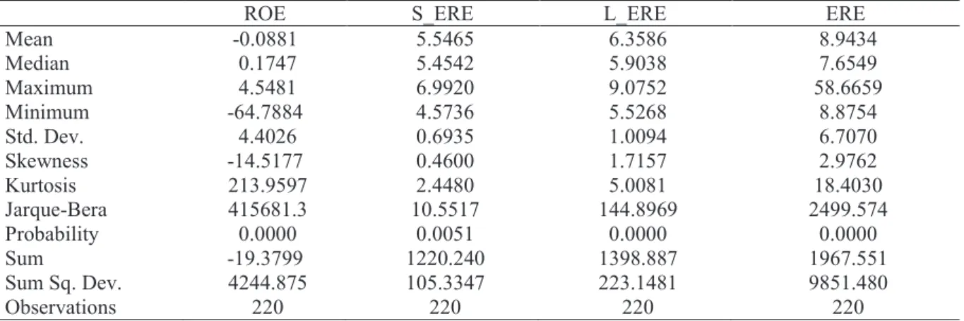
Table 1 illustrates vividly the descriptive statistics of the study variables. From the Table 1, it can be seen that all the equity risk exposure variables have positive means. However, returns accruing to the shareholders have negative mean. This is not strange considering that ROE takes its numerator value from net earnings which could assume negative values. The true averages of all the variables are positive. The true average here is denoted by the median as the variables do not have normal distribution. The results from the Jarque-Bera statistics indicate that the study rejects the null hypothesis that the series used in this study are drawn from a normally distributed random process. From Jarque-Bera test, when a variable has statistic with p-value of less than 0.05, then, the variable has no normal distribution and vice-versa. From the Table 1, all the variables have p-value of less than even 0.01 providing a strong case of no normal distribution. The p-values are the probability values below the Jarque-Bera statistics of each of the variables.
Following the literature since these variables are not normally distributed, the study uses median as the central tendency rather than the mean (Dess, Lumpkin & McFarlin, 2005). This means that the averages use in this study are based on the medians. Table 1 indicates that all the variables have positive medians. The averages (medians) are 0.1747, 5.4542, 5.9038 and 7.6549 for ROA, S_ERE, L_ERE and ERE respectively. The short term equity risk exposure (S_ERE) and long term equity risk exposure (L_ERE) have relatively low standard deviation (SD=0.6935 for S-ERE and 1.0094 for L_ERE). This shows that these variables have slow fluctuation or dispersions over the periods considered in this study. The standard deviation for total equity risk exposure (ERE) is 6.7070 and for return on equity (ROE) is 4.4026 is very high. These standard deviations suggest high level of fluctuation. The Table again reports the minimum and maximum values. The values for ROE, S_ERE, L_ERE and ERE are 4.5481(-64.7884), 6.9920(4.5736), 9.0752(5.5268) and 58.6659 (8.8754) respectively. The minimum values are in the parentheses. Whiles return on equity is negatively skewed; all the equity risk exposure variables have positive skewness. These suggest that the ROE has left tail whiles S_ERE. L_ERE and ERE are left tail. Apart from S_ERE with normal peakness, the rest of the variables have excess peakness. The details are on the Table below:
Table 1: Descriptive Statistics of the Study Variables
ROE S_ERE L_ERE ERE
Mean -0.0881 5.5465 6.3586 8.9434 Median 0.1747 5.4542 5.9038 7.6549 Maximum 4.5481 6.9920 9.0752 58.6659 Minimum -64.7884 4.5736 5.5268 8.8754 Std. Dev. 4.4026 0.6935 1.0094 6.7070 Skewness -14.5177 0.4600 1.7157 2.9762 Kurtosis 213.9597 2.4480 5.0081 18.4030 Jarque-Bera 415681.3 10.5517 144.8969 2499.574 Probability 0.0000 0.0051 0.0000 0.0000 Sum -19.3799 1220.240 1398.887 1967.551 Sum Sq. Dev. 4244.875 105.3347 223.1481 9851.480 Observations 220 220 220 220
Source: Generated from Eviews 7.0 Package 8.2 Panel Unit Root Analysis
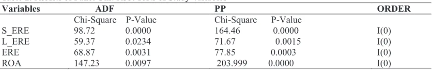
econometric estimations or specifically applying Ordinary Least Square. Since the study seeks to use panel ordinary least square estimator (POLS), it is crucial to determine the order of integration for reliable results (Froko, 2017). According to Froko (2017), when the stationarity assumption is not met a researcher could not appropriately estimate the study model at levels using OLS unless the series which have unit root be differenced. The paper tests the unit root assumption using Augmented Dickey Fuller (ADF) and Philip –Peron (PP). The results are reported in Table 2. It can be observed that all the variables are I(0). This means that the variables do not have unit root. It is also an indication that the variables are stationary and therefore POLS can be used to estimate the earnings model.
Table 2: Results of Panel Unit Root Tests of Study Variables
Variables ADF PP ORDER
Chi-Square P-Value Chi-Square P-Value
S_ERE 98.72 0.0000 164.46 0.0000 I(0)
L_ERE 59.37 0.0234 71.67 0.0015 I(0)
ERE 68.87 0.0031 77.85 0.0003 I(0)
ROA 147.23 0.0097 203.999 0.0000 I(0)
Source: computed using Eviews 7.0 Package 8.3 Hausman Test
One other diagnostics which is common for panel model specification is the choice between random and fixed effect. Researchers are confronted to make a choice of whether to use the random panel specification or fixed panel specifications. Although some researchers use qualitative characteristics as the basis for making such choice, such judgements may be erroneous as they could not be objectively be verified. One technique to make objective selection of suitable specification is the use of Hausman test. It is conducted on the null hypothesis that the appropriate specification is random effect. Therefore where the null hypothesis is rejected, then, it is concluded that fixed effect is the appropriate specification. However, when the study fails to reject this null hypothesis, the random effect becomes more suitable. The results are presented in Table 3. The Table shows that the study fails to reject the null hypotheses on cross-section random specification and the period random. Each of these tests generate p-values of 1.0000 each. Therefore, on individual basis either cross-section or period random requires random effect specification. However, the appropriate specification for estimating both cross-section and period effect together is the fixed effect.
Table 3: Hausman Chi-square Test on Equity Return Model
Test Summary Chi-Sq. Statistic Chi-Sq. d.f. Prob.
Cross-section random 0.000000 3 1.0000
Period random 0.000000 1 1.0000
Cross-section and period random 4.909934 1 0.0267
Source: Generated from Eviews 7.0 Package 8.4 Panel Estimation
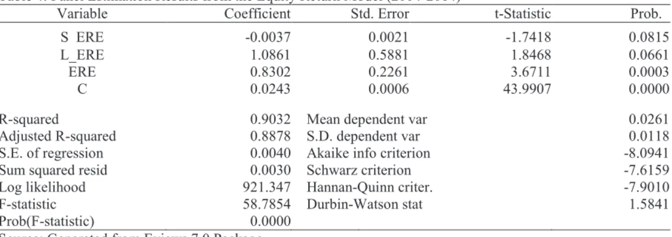
Having determined that it is more appropriate to employ two way fixed effect specifications, the study proceeds to estimate the returns model using such specification. The panel ordinary least square approach is used. The results are depicted in Table 4. The Table indicates that the R2 and adjusted R2 for the return model are 0.9032 and 0.8878 respectively. These statistics are usually used to determine the fitness or goodness of a model. The high the R2 and adjusted R2 values are good indication that the model estimated is good. The adjusted R2 of 0.8878 also suggests that holding other factors constant, the explanatory variables (capital structure indicator-Equity risk exposure) explain about 88.78% of variations in the level of returns on equity of banks in Ghana. The remaining 11.22% (100-88.78) is accounted for by factors outside this model. The model also shows significant f-statistic. The f-stat of 58.7854 has corresponding p-value of 0.0000. The f-stat indicates the coefficients of all the explanatory variables are jointly significant. The Durbin –Watson statistics is closer to 2 (1.5841) indicating that there is no autocorrelation. This provides further evidence of the strength of the model.
Table 4: Panel Estimation Results from the Equity Return Model (2004-2014)
Variable Coefficient Std. Error t-Statistic Prob.
S_ERE -0.0037 0.0021 -1.7418 0.0815
L_ERE 1.0861 0.5881 1.8468 0.0661
ERE 0.8302 0.2261 3.6711 0.0003
C 0.0243 0.0006 43.9907 0.0000
R-squared 0.9032 Mean dependent var 0.0261
Adjusted R-squared 0.8878 S.D. dependent var 0.0118
S.E. of regression 0.0040 Akaike info criterion -8.0941
Sum squared resid 0.0030 Schwarz criterion -7.6159
Log likelihood 921.347 Hannan-Quinn criter. -7.9010
F-statistic 58.7854 Durbin-Watson stat 1.5841
Prob(F-statistic) 0.0000
Source: Generated from Eviews 7.0 Package
It is observed from the Table 4 that the coefficient of short term equity risk exposure (S_ERE) is -0.0037. This coefficient is negative indicating that short term equity risk exposure has negative influence on equity returns. The p-value of this coefficient is 0.0815. This p-value is less than 10% demonstrating that the coefficient is significant. The implication is an increase in the level of short term equity risk exposure would decrease the equity return and vice-versa. It is therefore concluded that equity risk multiplier emanating from short term debt erode the equity returns of banks in Ghana
Contrary to this finding, the long term equity risk exposure has positive coefficient of 1.0861 with p-value of 0.0661. This coefficient is significant at 10%. Therefore, the study rejects the null hypothesis that long term equity risk exposure does not significantly affect equity return. It suggests that 1% increase in the level of long term equity risk exposure leads to 1.0861 increase in the level of equity return. On the other hand, a decrease in long term equity risk exposure could also reduce equity return.
The direction of the relationship between long term equity risk exposure and equity return is similar to the relationship between the total equity risk exposure (ERE) and equity return. The total equity risk exposure (ERE) in Table 4 has coefficient of 0.8302. The direction of this coefficient is positive indicating a positive influence on the level of equity return. The p-value of this coefficient is 0.0003. This means that the coefficient is significant. This suggests that the study rejects the null hypothesis of no significant effect of total equity risk exposure (ERE) on equity return at 1% confidence level.
The findings in summary are that equity risk exposure has significant relationship with equity return. Another finding from the analysis is that, the direction or nature of the effect of equity risk exposure on returns is based on time horizon of the exposure and the mixture of different time effect. Since this is the first time equity risk exposure has been conceptualised as component of capital structure, there are no empirical evidences in the literature to support or disaffirm the findings. However, the findings could be placed within the context of the theoretical literature so as to set the tone for further investigation. These findings are consistent with basic theory of intuition of investment. The basic theory of investment assumes that there is a positive relation between risk and returns. The higher the risk of an investment, the higher the returns should be and vice-versa. This is similar to the findings about the relationship between the equity risk exposure (total equity risk exposure and long term equity risk exposure) and the equity return.
The findings about total equity risk exposure and long term equity risk exposure also provide empirical evidence to support MM theory. One of the assumptions of the MM theory is that capital structure has positive effect on the expected return on equity arising from increasing earnings because the risk of equity increases with leverage (Modigliani & Miller, 1958). By implication, the MM theory suggests that equity risk exposure of capital structure positively affects the level of returns. In addition, the findings also provide empirical evidences to affirm the agency cost theory. The theory assumes that due to agency problem, shareholders or equity holders would ensure positive returns and subsequently rewarded for taking on extra risk. Therefore, per the agency cost theory, equity risk exposure is expected to have positive effect on return and this is consistent with the empirical results in this study.
To explain the negative significant effect of short term equity risk exposure on equity return, the financial distress and bankruptcy theory is employed. Following the financial distress and bankruptcy cost theory, increase in risk associated with debt financing such as equity risk of bankruptcy and ultimately decrease the returns (Harris & Raviv, 1991). The theory suggests that there is negative relationship between the level of equity risk exposure and returns which is similar to the significant negative predictive value of short term equity risk exposure to returns
The practical implication of the findings is that even though short term debts could generate high earnings through the high interest spread in the Ghanaian banking sector, equity return is safer only when there is
appropriate balance between equity risk arising from short term debt and long term. This defines the total equity risk exposure. Therefore, appropriate optimal risk exposure to maintain or increase equity return should have a mean statistics of 7.6549 (see Table 1). Pursuing a policy of accumulating customers’ deposits (short term debt)
without sustainable long term financial stability (long term debt) would not generate sustainable returns even though there would be high interest spread in favour of the banks in Ghana. The implication reflects the characteristics of the Ghanaian banking. Due to the poor investment culture, the accumulated deposits translated into loans may not generate the expected returns due to the cost of performing loan. These costs of non-performing loans could lead to financial distress and loss of equity value (equity risk exposure) if there is no long term financing (long term equity risk exposure). This extrapolation is evident by the recent UT Bank and Capital Bank scandal (BOG, 2017). Despite the high coverage, customers’ deposits and high public confidence, these
banks collapsed overnight due to high short term equity risk exposure arising from non-performing loans. UT banks won even banking award in 2011 and has been built through the banking class to the universal status.
According to Bank of Ghana (2017), the decision to liquidate these banks was to protect customers’ deposits.
This makes the short term equity risk exposure quite detrimental as found in this study.
Although the long term equity risk exposure is higher than the short term equity risk exposure, the direct implication on equity holders is long enough to generate positive returns to support the obligations of claims. Shareholders returns would not be exposed to panic withdrawal which is typical in the Ghanaian banking sector. Public reaction to bad news in the banking sector is swift. This makes short term equity risk difficult to accommodate and manage. The banks should therefore strive to balance their equity risk exposure between short term and long term as short term equity risk emanating from deposits mobilisation could undermine the returns sustainability of the equity holders.
9. Conclusion and Recommendation
This study examined how equity risk exposure emanating from capital structure decision determines proprietary value in the Ghanaian banking sector. The study conceptualised equity risk exposure into three components: short term equity risk exposure, long term equity risk exposure and total equity risk exposure. Since this is the first time this concept has been conceptualised within the framework of capital structure, the study was built based on theoretical evidences. The predictive relationship between the equity risk exposure and equity return was estimated using panel ordinary least square. It was found that short term equity risk exposure has negative influence on equity returns whiles long term equity risk exposure and total equity risk exposure generated positive influence. It was concluded that when the short term equity risk of banks in Ghana increases, they could sacrifice the equity returns (proprietary value) and vice-versa. Additionally, it was concluded that equity returns are likely to be improved when the equity risk is balanced between short term and long term debts. It was further revealed that long term equity risk sustains equity return better than short term equity risk exposure.
It is recommended that banks in Ghana should not be only concerned about mobilisation of short term debt (customers’ deposits) and generate income from these debts but also should be concerned about investment
vehicles that transform the mobilisation into better returns. This is critical as the study revealed that short term debt increases equity risk exposure and reduces proprietary value. Therefore, investing these funds in high risk investment may results in losing the equity value. This might have been one of the primary reasons that led to the collapsed of UT Bank and Capital Bank in Ghana. It is also concluded that although long term debt generates lower interest income compare to short term debt in Ghana, the long term has lower risk exposure than the short term debt. Therefore, management of banks in Ghana should strive to balance off the mixture of short term and long term debt to optimally reduce equity risk exposure and enhance proprietary value as found in this paper. References
1. Abor, J. (2005). The effect of capital structure on profitability: an empirical analysis of listed firms in Ghana. Journal of Risk Finance (Emerald Group Publishing Limited), 6(5), 438-445.
2. Amidu, M. (2007). Determinants of capital structure of banks in Ghana: an empirical approach. Baltic Journal of Management, 2(1), 67-79.
3. Bank of Ghana Report (2017), UT, Capital Bank Collapse: GCB to the Rescue. https://www.ghanaweb.com/GhanaHomePage/NewsArchive/UT-Capital-Bank-collapse-GCB-to-the-rescue-569424
4. Barclay, M. & Smith, C. (2005) Capital Structure Puzzle: The Evidence Revised. Journal of Applied Corporate Finance,17(1),8-17
5. Bayeh, A. K (2011) Capital Structure Determinants: An Empirical Study on Insurance Industry in Ethiopia. Addis Ababa University School of Graduate Studies
6. Brounen, D & Eichholtz, P A, (2001). Capital structure theory: Evidence from European property companies capital offerings’, Journal of Real Estate Economics, 2, pp. 4-21.
Japanese Manufacturing Companies. Journal of International Business Research, 11(3); 1-15.
8. Frank M.Z. & Goyal V. .K. (2003) Testing the pecking order theory of capital structure, Journal of Financial Economics, 67, p.p. 217-248.
9. Goyal, A. M. (2013). Impact of capital structure on performance of listed public sector banks in India. International Journal of Business and Management Invention, 2(10), 35-43.
10. Harris, M., & Raviv, A. (1991), The Theory of Capital Structure, Journal of Finance, 46, 297-355
11. Jensen, M. and Meckling, W. (1976), “Theory of the firm: managerial behavior, agency costs and Ownership structure”, Journal of Financial Economics, 3, 305-60.
12. Kyereboah-Coleman, A. (2007). The impact of capital structure on the performance of microfinance institutions. [Article]. Journal of Risk Finance (Emerald Group Publishing Limited), 8(1), 56-71.
13. Modigliani F & Miller M. (1958), The cost of capital Corporate finance and the theory of investment”,
American Economic Review, 48, pp. 261-297.
14. Muhammad, U. Z., Tanveer, S. A., & Muhammad, S., (2012). Impact of Capital Structure on Firms’
Financial Performance: Evidence from Pakistan. Research Journal of Finance and Accounting , 3(9), 15. Myers C.S. (1984), The capital structure puzzle The Journal of Finance, 39 (3), 575 - 592.
16. Olokoyo, F.A., (2012) capital structure and corporate performance of Nigerian quoted firms: a panel data approach. Ph.D thesis Covenant University, Ota, Ogun state, Nigeria.
17. Queku, I. C. (2017) Value Relevance of International Financial Reporting Standards (IFRS) and
Shareholders’ Wealth Maximisation: Evidence from Banks in Ghana. Accepted for publication: International Journal Advanced Research (IJAR),
18. Ross, W & Jaffe, J (2011). Core principles and applications of corporate finance. Global edition
19. San, T. O & Heng, B. T (2011), Capital Structure and Corporate Performance of Malaysian Construction
Sector”, International Journal of Humanities and Social Sciences, 1(2), 28-36.
20. Tianyu, H (2013). The comparison of impact from capital structure to corporate performance between Chinese and European listed firms. Jonkopon International Business School, Jonkopon university
21. Froko, N. A. (2017) Short term financial leverage and shareholders’ wealth maximisation of Ghanaian