Coordinated Tax-Tariff Reforms, Informality,
and Welfare Distribution
Jenny E. Ligthart
Gerard C. van der Meijden
CES
IFO
W
ORKING
P
APER
N
O
.
3107
CATEGORY 1: PUBLIC FINANCE
JUNE 2010
An electronic version of the paper may be downloaded • from the SSRN website: www.SSRN.com • from the RePEc website: www.RePEc.org • from the CESifo website: Twww.CESifo-group.org/wpT
CESifo
Working Paper No. 3107
Coordinated Tax-Tariff Reforms, Informality,
and Welfare Distribution
Abstract
The paper studies the revenue, efficiency, and distributional implications of a simple strategy
of offsetting tariff reductions with increases in destination-based consumption taxes so as to
leave consumer prices unchanged. We employ a dynamic micro-founded macroeconomic
model of a small open developing economy, which features an informal sector that cannot be
taxed, a formal agricultural sector, and an import-substitution sector. The reform strategy
increases government revenue, imports, exports, and the informal sector. In contrast to Emran
and Stiglitz (2005), who ignore the dynamic effects of taxes and tariffs on factor markets, we
find an efficiency gain, which is unevenly distributed. Existing generations benefit more than
future generations, who - depending on pre-existing tax and tariff rates and the informal
sector size - even may become worse off.
JEL-Code: E26, F11, F13, H20, H26.
Keywords: tariff reform, consumption tax reform, informal sector, home production,
transitional dynamics, overlapping generations, second-best outcome.
Jenny E. Ligthart
Department of Economics and CentER
Tilburg University
P.O. Box 90153
5000 LE Tilburg
The Netherlands
j.ligthart@uvt.nl
Gerard C. van der Meijden
Department of Economics and CentER
Tilburg University
P.O. Box 90153
5000 LE Tilburg
The Netherlands
g.c.vdrmeijden@uvt.nl
May 2010
The authors would like to thank Pedro Bom, Bas van Groezen, Ben Heijdra, and the
participants of the 2010 NAKE Research Day at Utrecht University for helpful comments.
1
Introduction
Tariff revenue of low-income countries has declined from 5.4 percent of GDP in 1985 to 3.4 percent of GDP in 2000, which is primarily driven by their trade liberalization programs. Nevertheless, trade taxes continue to be the major source of revenue for these nations: tariff revenue accounted on average for 30 percent of total tax revenue during 1990–2000 compared with only 1 percent in OECD countries.1 Washington-based financial institutions such as the International Monetary Fund (IMF) and the World Bank have strongly advocated tariff cuts coupled with tax measures to recoup the potential public revenue losses. Much of the discussion on alternative revenue sources has focused on consumption taxes like the value-added tax (VAT). Policy prescriptions of the IMF and the World Bank are typically based on the (presumed) efficiency gain of these integrated tax-tariff reforms. Recently, Emran and Stiglitz (2005) have challenged the validity of this prescription by pointing to the efficiency loss induced by the presence of a “hard-to-tax” informal sector.2 Our paper contributes to this debate. More specifically, we show that the Washington-based policy line remains valid—even when a substantial informal sector exists—once allowance is made for factor market dynamics. There is a large informal literature discussing potential measures to offset the revenue loss of tariff reform. See, for example, Mitra (1999). Early theoretical analyses primarily focus on the welfare effects of tariff cuts (cf. Hatta, 1977). Such tariffs cuts, however, typically imply a tariff revenue loss for developing countries. The sparse literature on coordinated tax-tariff reforms acknowledges countries’ budget constraints and studies tax measures to offset the associated revenue losses. Early contributions are those by Hatzipanayotou et al. (1994) and Keen and Ligthart (2002), who find that integrated tax-tariff reforms increase both government revenue and welfare.3 Intuitively, the reform reduces the static implicit production subsidy at an unchanged consumption tax distortion. Recently, the desirability of integrated reform strategies has been under discussion. The main result may break down when allowance is made for important features of reality such as an informal sector (cf. Emran and Stiglitz, 2005), imperfect competition on the goods market (cf. Haque and Mukherjee, 2005; and Keen and Ligthart, 2005), and tax administration costs (cf. Munk, 2008). The existing literature typically employs static (partial) equilibrium frameworks to analyze piecemeal tax-tariff reforms and thus can neither take into account important effects on domestic factor markets nor consider transitional dynamics.4
1
See Ebrill, Stotsky, and Gropp (1999) and World Bank (2009). Income groups are defined by the World Bank classification.
2
See Schneider and Enste (2000) for an overview of the size, causes, and economic consequences of informal sector activities.
3Boadway and Sato (2009) take a different perspective by constructing a general model of optimal tax
design in an economy with an informal sector. They compare a VAT regime with a trade tax regime and identify the circumstances that determine which of the two is preferred on efficiency grounds.
4
Notable exceptions are Naito (2006) and Heijdra and Ligthart (2010). Their models neither feature an informal sector nor allow for distributional issues.
Our work is most closely related to Emran and Stiglitz (2005), who acknowledge the incomplete coverage of VAT due to the existence of an informal sector. Employing a model with fixed factor endowments, they investigate the welfare effect of an integrated tax-tariff reform so as to leave government revenue unchanged. While a radial tariff reduction is shown to alleviate both consumption and production distortions, the revenue-neutral increase in the VAT reinforces the consumption distortion across formal and informal sectors.5 Emran and Stiglitz (2005) find that such a reform reduces welfare under plausible conditions, leading them to conclude that ‘...the results derived earlier in the literature are unhelpful at best and potentially misleading as the basis of indirect tax policy reform in developing countries’ (Emran and Stiglitz, 2005, p. 618).6 However, although Emran and Stiglitz (2005) take into account the static output distortion induced by the import tariff, their model ignores the dynamic distortion of the tariff. In a dynamic setting, tariffs affect firms’ investment decisions and thereby the accumulation of physical capital. Given that import-competing sectors are typically much more capital intensive than the rest of the economy (including the informal sector), the import tariff is relatively more distorting compared to the consumption tax than it is in the static analysis of Emran and Stiglitz (2005).
This paper studies the revenue, efficiency, and intergenerational welfare effects of a reform strategy of cutting tariffs and increasing destination-based consumption taxes so as to leave domestic consumer prices unchanged. To this end, we construct a dynamic macroeconomic model of a small open developing economy. Our analysis explicitly considers an informal sector and factor market dynamics. The strategy of keeping consumer prices fixed allows us to focus on the effects of a change in the composition of the combined burden of consumption taxes and tariffs rather than the level of the tax burden, implying that all efficiency gains/losses from the reform materialize as a change in the market value of aggregate consumption. Besides being analytically simple, this strategy is also practical. Compared with a revenue-neutral reform—which requires an analysis of time-varying consumption tax rates—all that is needed is information on the current marginal tariff and tax rates.
We consider a model in which households are finitely lived, building on the work of Yaari (1965) and Blanchard (1985). In line with the economic structure of a typical developing country, households engage in home production.7 Because of measurement problems, this kind of informal output neither enters the national accounts nor can be taxed (cf. Tanzi, 1999). The home production specification builds on the real business cycle (RBC) literature
5
Emran and Stiglitz’s (2005) analysis concerns the case of a selective tax-tariff reform, which contrary to a radial reform only applies to a subset of the commodities subject to the tax and the tariff. However, they claim that the results go through for a radial reform, which they work out in an (unpublished) paper.
6
Keen (2008) argues that Emran and Stiglitz (2005) underestimate the extent to which the VAT is able to tax the informal sector, because the VAT functions as a tax on the purchases (including imports) of firms in the informal sector (which cannot claim an input tax credit).
7
As Schneider (2002, p. 30) notes, informal activities in developing countries are primarily related to household production.
(cf. Benhabib, Rogerson, and Wright, 1991; Parente, Rogerson, and Wright, 2000; and Campbell and Ludvigson, 2001).8 In our framework, firms operate in two market sectors, that is, an export sector and an import-substitution sector. Following Brock and Turnovsky (1993), the export sector produces an agricultural good using labor and a sector-specific factor (land), whereas the import-substitution sector produces a manufactured good employing labor and imported physical capital as a sector-specific factor. Both goods and factor markets are perfectly competitive. Labor is perfectly mobile across the informal and formal sector and within the formal sector.9 To avoid trivial capital dynamics, capital accumulation is subject to adjustment costs.
We solve the model analytically and provide numerical illustrations of the transitional allocation effects and welfare effects of a tax-tariff reform. To this latter end, we simulate the model for empirically plausible parameter values. The reform strategy is shown to increase government revenue and market access in the long run, that is, steady-state imports and exports rise.10 In addition, both the informal and formal agricultural sector expand at the
expense of the import-substitution sector; however, informal agricultural output rises rela-tively more. Aggregate formal employment and output fall, more so in the long run than in the short run. The qualitative allocation effects are robust to changes in the size of the informal sector. In contrast to Emran and Stiglitz (2005), we find an efficiency gain under plausible conditions. Intuitively, the reform alleviates the tariff distortion (yielding too much production and too little consumption of import substitutes) more than it exacerbates the consumption tax distortion (giving rise to excess home production). More specifically, in addition to a static efficiency gain, lower tariff rates also generate an intertemporal efficiency gain; that is, tariffs reduce the larger than socially optimal physical capital stock in the import-substitution sector. The welfare change is unequally distributed across generations. Old existing generations benefit more than young generations. Future generations may even become worse off, depending on the pre-existing tax and tariff rates and the share of informal output in GDP.
The paper proceeds as follows. Section 2 sets out a micro-founded model of a small open economy extended with an informal sector. Section 3 describes the solution procedure. Sec-tion 4 studies the dynamic allocaSec-tion effects of a consumer-price neutral tax-tariff reform strategy in which tariffs on imported consumption goods are lowered and destination-based consumption taxes are increased. Section 5 studies the dynamic efficiency and
intergenera-8
Pigott and Whally (2001) investigate a VAT base broadening while allowing for household production. However, they do not consider tariffs and calibrate their model for Canada. Turnovsky and Basher (2009) employ a dynamic macroeconomic model in which firms rather than households produce informal goods. They focus on a closed economy and therefore do not touch upon tariff reform issues.
9
We use the terms home production, informal sector, and shadow economy interchangeably.
10
Anderson and Neary (2007) show that welfare-improving tariff reforms in general do not coincide with market access-improving tariff reforms. Nevertheless, Kreickemeier and Raimondos-Møller (2008) succeed in deriving a revenue-neutral tax-tariff reform that increases welfare, market access, and government revenue.
tional welfare effects. Section 6 concludes.
2
The Model
This section sets out the dynamic micro-founded model of a small open developing country. We subsequently discuss behavior of individual households, aggregate households, firms, and the government.
2.1 Individual Households
Following Yaari (1965) and Blanchard (1985), individual households face a constant proba-bility of deathβ >0, which equals the rate at which new agents are born. Consequently, the population size is constant and can thus be normalized to unity. Households are disconnected and therefore do not leave bequests. Actuarially fair annuity markets allow households to bor-row and lend funds at the exogenously given world rate of interest adjusted for the probability of death.
Expected lifetime utility at time t of a representative household born at time v ≤ t is given by the following additively separable specification:
Λ(v, t) =
Z ∞
t
lnC(v, z)e−(ρ+β)(z−t)dz, (1)
where ρ is the pure rate of time preference. Consumption is discounted at the effective discount rate ρ+β, reflecting the positive death rate. The aggregate consumption index
C(v, t) is given by:
C(v, t)≡CM(v, t)εCA(v, t)1−ε, 0< ε <1, (2)
which is defined over a manufactured good CM(v, t) and a composite agricultural good
CA(v, t). The parameterεrepresents the consumption share of manufactured goods.
House-holds can either choose to buyCE(v, t) agricultural goods on the market or produce CS(v, t)
of these goods at home:11
CA(v, t)≡CE(v, t) +CS(v, t). (3)
The household allocates its total time available, which we have normalized to unity, be-tween working LF(v, t) hours in the market sector and working LS(v, t) hours at home
(so-called informal employment). The household’s home production function is given by:
CS(v, t) =YS(v, t) = ΩSLS(v, t)1−αS, 0< αS<1, ΩS >0, (4)
11
This specification is warranted because home and market goods are typically close substitutes in developing countries (Parente, Rogerson, and Wright, 2000, p. 683).
where ΩS is a productivity index, YS(v, t) is home production, and 1−αS is the output
elasticity of time devoted to home production. Equation (4) says that home production of generationvis fully consumed by the representative household of that generation. Allimplicit income earned in the informal sector is attributed to labor.
The household’s flow budget constraint is: ˙
A(v, t) = (r+β)A(v, t) +w(t)LF(v, t) +T(t)−pM(t)CM(v, t)−pE(t)CE(v, t), (5)
where ˙A(v, t)≡dA(v, t)/dt,A(v, t) denotes real financial wealth,ris the world rate of interest,
w(t) is the (age-independent) real wage rate,LF(v, t) is total employment in the market sector,
T(t) are lump-sum transfers, pM(t) is the domestic consumer price of manufactured goods,
andpE(t) is the domestic consumer price of agricultural goods produced in the export sector.
We choose the exported agricultural good as the numeraire. The world market prices of agricultural and manufactured goods are exogenously given. Hence, we can normalize them to unity. The domestic consumer prices of manufactured and agricultural goods produced in the market are defined as:
pM(t)≡(1 +tC(t))(1 +τM(t)), pE(t)≡1 +tC(t), (6)
whereτM(t) is an ad valorem import tariff on imported manufactured goods andtC(t) denotes
an ad valorem destination-based consumption tax (which is applied to the tariff-inclusive import price, in line with international practice).
The representative household of cohortv chooses time profiles forCM(v, t),CE(v, t), and
CS(v, t) to maximize Λ(v, t) subject to its flow budget constraint (5), the home production
function (4), and a No-Ponzi-Game solvency condition. By solving this optimization problem, we find the following three necessary conditions:
ε 1−ε CA(v, t) CM(v, t) = pM(t) pA(t) , (7) pA(t)(1−αS)ΩSLS(v, t)−αS = w(t), (8) ˙ X(v, t) X(v, t) = r−ρ, (9)
where pA(t) is the price index of composite agricultural consumption and full consumption
X(v, t) is defined as the market value of aggregate consumption:
X(v, t)≡pC(t)C(v, t) =pM(t)CM(v, t) +pA(t)CA(v, t), (10)
wherepC(t) is thetrue price index of the aggregate consumption index:
pC(t) = ΦCpM(t)εpA(t)1−ε, ΦC ≡
εε(1−ε)1−ε−1
>0. (11)
Because CE(v, t) and CS(v, t) are perfect substitutes, the shadow price of home production
Condition (7) sets the marginal rate of substitution between agricultural goods and imported goods equal to their relative price. Equation (7) says that the value of the marginal product of time devoted to informal activities should be equal to the real market wage rate. According to (8), optimal individual full consumption growth is given by the difference between the real interest rate and the pure rate of time preference. We consider the case of a patient nation for whichr > ρholds. By integrating (5), and using (8) and (10), it follows that full consumption of the representative household is a fixed fraction of total wealth:
X(v, t) = (ρ+β) [A(v, t) +H(v, t)], (12)
whereH(v, t) is the expected lifetime human wealth of vintagev at time t:
H(v, t)≡
Z ∞
t
[w(z)LF(v, z) +T(z) +pS(z)YS(v, z)]e−(r+β)(z−t)dz, (13)
which equals the expected discounted value of the current and future returns to labor, which consists of formal wage income, lump-sum transfers, and all implicit income earned in the shadow economy.
2.2 Aggregate Household Sector
Aggregate variables can be calculated from the individual variables by integrating over all existing generations while noting that in each period the number of newbornsβ is equal to the number of households that pass away. We assume large cohorts, so that frequencies and probabilities coincide by the law of large numbers. Therefore, aggregate full consumption, for example, is given by:
X(t)≡
Z t
−∞
βX(v, t)eβ(v−t)dv. (14)
The aggregate values for other variables can be derived in a similar fashion. By taking the time derivative of (14), the aggregate version of (8) is obtained:
˙ X(t) X(t) =r−ρ−β(ρ+β) A(t) X(t) = ˙ X(v, t) X(v, t)−β X(t)−X(t, t) X(t) . (15)
Aggregate full consumption growth differs from individual full consumption growth because of the generational turnover effect (cf. Heijdra and Ligthart, 2007). On the one hand, the birth of new generations has a positive effect on aggregate consumption growth (represented by the term βX(t, t) on the right-hand side of the second equality sign). On the other hand, the death of old generations has a negative effect on aggregate growth, reflecting that they cease to consume (represented by the term −βX(t)). Because old generations are wealthier than newborn households, they consume more. Consequently, on balance, aggregate full consumption growth falls short of individual full consumption growth.
Aggregate informal output is given by:
YS(t) =
Z t
−∞
βYS(v, t)eβ(v−t)dv. (16)
Because the real wage rate is the same for every generation, it follows from (7) that the level of individual informal production is independent of the household’s age. Hence, we know that individual informal production and aggregate informal production coincide: YS(t) =
YS(v, t).12
2.3 Firms
Production of market goods takes place in an agricultural sector and a manufacturing sector. Formal agricultural firms produce predominantly for the export market, but also sell products on the domestic market. Domestic manufacturing firms compete with foreign firms that produce a perfect substitute for the manufactured commodity. Both sectors are perfectly competitive, yielding zero excess profits.
2.3.1 Export Sector
Output in the export sector YE(t) is produced according to the following Cobb-Douglas
pro-duction function:
YE(t) = ΩEZEαELE(t)1−αE, 0< αE <1, ΩE >0, (17)
where ΩE is a productivity index,LE(t) is employment in the export sector,ZE denotes the
fixed factor land, and 1−αE is the output elasticity of labor in the agricultural sector. The
representative firm in the export sector maximizes its net operating surplus:
ΠE(t)≡YE(t)−w(t)LE(t)−rZ(t)ZE, (18)
whererZ(t) is the rental rate on land. We assume that the government cannot tax land.13
The first-order conditions characterizing the firm’s optimal plans are
w(t) = (1−αE)ΩE ZE LE(t) αE , rZ(t) =αEΩE ZE LE(t) −(1−αE) . (19)
The first expression yields the labor demand curve in the export sector. The land rentals— which are distributed to households—are equal to the firm’s gross operating surplus, that is,
¯
ΠE(t) =αEYE(t) =rZ(t)ZE.
12
Aggregate variables and variables averaged over all generations are equal, because of the normalization of the population size to unity.
13
If the government were to have access to a land tax—which is a non-distortionary source of revenue given that land is a fixed factor—then it becomes hard to justify why the government employs distortionary tariffs and consumption taxes.
2.3.2 Import-Substitution Sector
The representative firm in the import-substitution sector produces YM(t) according to a
Cobb-Douglas technology:
YM(t) = ΩMK(t)αMLM(t)1−αM, 0< αM <1, ΩM >0, (20)
where ΩM is a productivity index, LM(t) is employment in the import-substitution sector,
K(t) denotes the physical capital stock, and αM is the output elasticity of physical capital
in the manufacturing sector. Capital goods can only be imported, do not bear any tariff or tax, and are subject to adjustment costs. Following Uzawa (1969), the firm faces a strictly concave accumulation function Ψ(·) that links net capital accumulation to gross investment:
˙ K(t) = Ψ I(t) K(t) −δ K(t), (21)
where δ >0 is the constant rate of capital depreciation and I(t) denotes gross investment. The accumulation function has the following properties: Ψ(0) = 0, Ψ0(·)>0, and Ψ00(·)<0.
Because of adjustment costs, physical capital is less mobile in the short run than in the long run. The degree of physical capital immobility is given by σ ≡ −(I/K)Ψ00/Ψ0 >0, where a smallσ characterizes a high degree of capital mobility. Note that the limiting case of σ →0 (i.e., no adjustment costs) corresponds to perfect capital mobility.
The firm chooses employment and investment to maximize its stock market value,
VK(t)≡
Z ∞
t
[(1 +τM(z))YM(z)−w(z)LM(z)−I(z)]e−r(z−t)dz, (22)
subject to the production function (20), the accumulation equation (21), and a transversality condition: limz→∞q(z)K(z)e−r(z−t) = 0, where q(t) denotes Tobin’s q, which measures the
market value of physical capital relative to its replacement costs. The firm takes the (positive) initial stock of physical capital as given. We have normalized the price of imported capital goods to unity. The optimization procedure yields the following first-order conditions:
w(t) = (1 +τM(t))(1−αM)ΩM K(t) LM(t) αM , (23) 1 = q(t)Ψ0 I(t) K(t) , (24) ˙ q(t) + (1 +τM(t))αMYKM((tt)) q(t) =r+δ− Ψ I(t) K(t) −Ψ0 I(t) K(t) I(t) K(t) . (25)
Equation (23) yields labor demand conditional on the physical capital stock. Investment demand is given by (24), which is a positive function of Tobin’sq. Equation (25) describes the evolution of Tobin’sq, which ensures that the return on physical capital (the left-hand side) equals the user costs of physical capital (the right-hand side). The return on physical capital is the sum of the shadow capital gains/losses and the marginal product of capital. The
user costs of physical capital consist of the interest rate, the depreciation rate, and the term between brackets, which captures the effect of investment on future adjustment costs. Because the adjustment function is strictly concave, the bracketed term is positive. Intuitively, current investment increases the future capital stock, thereby lowering future adjustment costs.14
2.4 Government
The government levies taxes on consumption in the formal sector, but cannot tax consumption of informal goods.15 In addition, the government imposes tariffs on imported consumption goods. In line with international practice, all consumption taxes are destination-based, im-plying that exported goods are zero-rated and imported goods are taxed. The government distributes tax revenues to households in a lump-sum fashion. Hence, the government’s budget identity is given by:
T(t) =tC(t) [CE(t) + (1 +τM(t))CM(t)] +τM(t)[CM(t)−YM(t)]. (26)
The first term on the right-hand side of (26) represents consumption tax revenue, where we take into consideration that consumption taxes are levied on the domestic consumption of
CE(t) and the tariff-inclusive value of CM(t). The second term denotes tariff revenue from
imported consumption goods.
2.5 Foreign Sector
Given the relative market prices, the small open economy importsXM(t) = CM(t) +I(t)−
YM(t) of the manufactured good and exportsXE(t) =YE(t)−CE(t) of the formal agricultural
good. The trade account of the balance of payments is obtained by subtracting imports from exports: XE(t)−XM(t) =YM(t) +YE(t)−[CM(t) +CE(t) +I(t)], showing that market output
YM(t) +YE(t) less domestic (market) absorptionCE(t) +CM(t) +I(t) equals aggregate net
exports. The evolution of net foreign assets is then given by: ˙
F(t) =rF(t) +XE(t)−XM(t). (27)
National solvency is retained provided the initial value of net foreign assets equals the present value of trade account deficits:
F(t) =−
Z ∞
t
[XE(z)−XM(z)]e−r(z−t)dz. (28)
14Without adjustment costs, we have Ψ (·) =I(t)/K(t), which yieldsσ= 0. Equation (24) then reduces to q= 1. In this case,q(t) andK(t) adjust instantaneously to their steady-state levels. Consequently, equation (25) collapses to (1 +τM)∂Y∂KM =r+δ,which is the familiar rental rate derived in a static framework.
15Tax evasion in the informal sector is assumed to be 100 percent. We thus abstract from the possibility of
2.6 Market Equilibrium
Equilibrium in the goods market is given by: YM(t) +YE(t) +XM(t) = CM(t) +CE(t) +
I(t) +XE(t), where the right-hand side shows the sources of aggregate demand. We define
the country’s Gross Domestic Product (valued at domestic market prices) as: Y(t) = (1 +
tC(t))[(1 +τM(t))YM(t) +YE(t)]. In line with international practice, official GDP does not
include any output produced in the informal economy.
Labor market equilibrium requires that LF(t) +LS(t) = 1, where aggregate formal
em-ployment is LF(t) = LE(t) +LM(t) and aggregate informal employment is LS(t). Because
informal employment is inversely related to the wage rate and total time is normalized to unity, aggregate formal employment rises with the wage rate. Financial market equilibrium implies that household’s aggregate claim on assets equals the sum of the value of the domestic physical capital stockVK(t), the value of the stock of landVZ(t), and net foreign assets:
A(t) =VK(t) +VZ(t) +F(t). (29)
The stock market value of import-competing firms is given byVK(t)≡q(t)K(t). All financial
assets are assumed to be perfect substitutes. Arbitrage ensures that land attracts the market rate of return, which consists of the sum of the capital gain ˙VZ(t) and the rental rate rZ(t):
rVZ(t) = ˙VZ(t) +rZ(t), (30)
where we have normalized the constant stock of land to unity, that is,ZE = 1.
3
Solving the Model
This section solves the model, describes its dynamic properties, and discusses the parameters used in the numerical simulations of Sections 4 and 5.
3.1 Steady State
To analyze the dynamic properties of the model, we log-linearize it around an initial steady state (Table A1). A tilde (˜) denotes a relative change for most variables (e.g., ˜X(t) ≡
dX(t)/X), except for financial variables, lump-sum transfers, tax rates, and tariffs rates (see Appendix A.1 for a further discussion). Time derivatives of variables are generally defined asX˙˜(t)≡X˙(t)/X. The model can be reduced to a four dimensional dynamic system, which consists of two predetermined variables [ ˜K(t),A˜(t)] and two non-predetermined or forward-looking variables [˜q(t),X˜(t)]. Because the dynamic system is recursive, the investment sub-system [˜q(t),K˜(t)] can be solved independent of the savings subsystem [ ˜X(t),A˜(t)]. The model is locally saddle-point stable; its stability properties are summarized in Proposition 1.
Proposition 1 The model is locally saddle-point stable ifr < ρ+ηβ, where0< η ≡[1 + (1−
ε)τM]/[(1+tC)(1+τM)]<1. The dynamic system can be decomposed in two subsystems—one
for investment and one for savings—with the following properties:
(i) the investment system has two distinct real eigenvalues; that is, −h∗1 < 0 and r∗1 =
h∗1+r >0 with∂h∗1/∂σ <0, limσ→0h∗1 =∞, andlimσ→∞h∗1 = 0; and
(ii) the savings system has two distinct real eigenvalues; that is, −h∗2 < 0 and r∗2 = h∗2+ 2r−ρ >0 with∂h∗2/∂β >0 and limβ→∞h∗2=∞.
Proof. See Appendices A.2 and A.3.
Deferring technical details to Appendix A.2 and dropping time indices, the investment system can be written as:
" ˙˜ K ˙˜ q # = " 0 δ12 δ21 r # " ˜ K ˜ q # + " 0 0 −λq γq # " ˜ τM ˜ tC # , (31) where δ12 ≡ rωI/(σωK) > 0, δ21 ≡ r(ωLM)2αMαSαE/(|Ω|ωK) > 0, and |Ω| = αMαEωLS+
αSαEωLM +αSαMωEL > 0 is the determinant of the Jacobian matrix corresponding to the
labor market equilibrium (Appendix A.1). The GDP shares of the respective variables are defined as: ωI ≡ I/Y, ωK ≡rqK/Y, and ωLi =wLi/Y for i={M, E, S}. The elements in
the matrix of tax policy shocks are given by:
λq≡ αM 1−αM rωML ωK αEωSL+αS ωLE+αEωLM |Ω| >0, γq≡ r ωLM ωK αMαEωSL |Ω| >0,
and the shock terms are defined as ˜τM ≡dτM/(1+τM) and ˜tC ≡dtC/(1+tC). The investment
system can be graphically summarized by the phase diagram in Panel (a) of Figure 1. The ˙˜
K= 0 line represents combinations of ˜q and ˜K for which net investment is zero. The schedule is horizontal at ˜q∗ = 0, which corresponds to the steady-state value of Tobin’s q for which Ψ(.) = δ. ˜q-values exceeding ˜q∗ yield positive net investment. Conversely, ˜q-values falling short of ˜q∗ give rise to negative net investment, which is indicated by the horizontal arrows in the figure. The ˙˜q = 0 schedule is downward sloping and shows combinations of ˜q and
˜
K for which Tobin’s q is constant over time. Intuitively, a higher capital stock leads to a fall in the marginal product of capital and thus yields lower dividends to shareholders. For points to the right of the ˙˜q = 0 schedule, the marginal product of capital is too low, so that part of the return to capital consists of capital gains. Conversely, for points to the left of
˙˜
q = 0 schedule, the the marginal product of capital is too high, giving rise to capital losses on investment. Hence, ˙˜q >0 to the right of the line and ˙˜q <0 to the left, as represented by
Figure 1: Phase Diagrams: The Investment and Savings System Panel (a): Investment System
q K 0 [q=0] 1 [q=0] 0 K= 0 E 1 E A 1 SP 0 SP
Panel (b): Savings System
A X 0 X = 1 [A=0] 0 [A=0] [A 0] ∞ = i i i 0 E A E∞ 1 SP 0 SP SP ∞ iB
Notes: Panel (b) describes a special case of the model, corresponding to the benchmark calibration. The financial wealth
schedule shifts up at impact and remains above its initial position if and only ifεγA−λA >0 andκA(εγq+λq)−
the vertical arrows in Figure 1. The arrow configuration confirms that the equilibrium at E0
is saddle-point stable.
Again relegating the derivations to the appendix, the savings system can be written as:
" ˙˜ X ˙˜ A # = " r−ρ −rω−ρ A −rηωX r # " ˜ X ˜ A # + " 0 0 0 κA λA γA # ˜ K ˜ τM ˜ tC , (32)
where ωX ≡ X/Y, ωA ≡ rA/Y, and the composite terms κA, λA, and γA are defined in
Appendix A.3. Pre-existing tax and tariff rates and the relative sector sizes determine the signs of these terms. Because the system features the capital stock in the second vector on the right-hand side of (32), the first shock term is time-varying. The savings system is graphically represented in Panel (b) of Figure 1. The X˙˜ = 0 line represents combinations of ˜X and ˜A for which aggregate full consumption does not change. The schedule is upward sloping, owing to the generational turnover effect; that is, larger financial wealth holdings by households increase the gap between consumption of newborn generations and aggregate full consumption so that aggregate full consumption must increase to keep the proportional gap constant. If financial wealth exceeds the equilibrium value, full consumption declines. Conversely, if financial wealth falls short of the equilibrium value, full consumption increases. TheA˙˜= 0 locus depicts combinations of ˜Xand ˜Afor which financial wealth is constant. This schedule is also upward sloping, because an increase in financial wealth supports a higher level of full consumption. The slope of the X˙˜ = 0 line is steeper with respect to the ˜A axis than that of theA˙˜= 0 schedule. For points above theA˙˜= 0 schedule, full consumption is too high, leading to a decrease in financial wealth. Conversely, for points below the A˙˜ = 0 schedule, financial wealth rises. As can be inferred from the arrow configuration, the equilibrium is saddle-point stable.
3.2 Calibration
To get insight into the quantitative allocation and welfare effects, we calibrate the model to match a typical low-income developing economy by using parameter values taken from the literature and derived from primary data. Table 1 provides an overview of the chosen parameter values. We set the world interest rate r to 4 percent (cf. Mendoza, 1991). We choose a value ofβ= 0.033 to match the average crude birth rate—which is assumed to equal the death rate—in low-income countries over the last decade (World Bank, 2009), implying an average expected working lifetime of 33.33 years. In order to get a reasonable imports-to-GDP share, the taste parameterε is set to 0.55.
In line with Gollin (2002), we set the output elasticity of labor in the import-substitution sector 1−αM to 0.67. Based on Valentinyi and Herrendorf (2008), who find that the labor
income share in the agricultural sector is lower than that of the aggregate economy because of the large land income share, we use 1−αE = 0.5. We assume that the production elasticity
T able 1: The P arameter V alues in the Benc hmark Mo del Description P arameter V alue Source Pr efer enc es ε 0.550 W orld Bank (2009), World Development Indic ators Demo gr aphy β 0.033 Av erage exp ected life span of 33.3 w orking y ears World inter est rate r 0.040 Mend oz a (1991) T echnolo gy αE 0.500 V alen tin yi and Herrendorf (2008) αM 0.330 Gollin (2002) αS 0.500 V alen tin yi and Herrendorf (2008) ΩE 1.000 W orld Bank (2009), World Development Indic ators ΩM 0.750 W orld Bank (2009), World Development Indic ators ΩS 0.850 Sc hneider and Enste (2002) and P aren te , Rogerson, and W righ t (2000) Capital ac cumu lation δ 0.100 Mend oz a (1991) and Mendoza and T esar (2005) ¯ z 1.250 Mend oz a (1991) T ax rates tC 0.125 Gord on and Li (2009) τM 0.200 E brill, Stotsky , and Gropp (1999)
of labor in home production 1−αS also takes on a value of 0.5. The productivity indexes are
chosen to get empirically plausible sectoral output levels as share of GDP. In keeping with the RBC literature (cf. Kydland and Prescott, 1982), the rate of depreciationδis set to 0.10. We employ a logarithmic specification of the concave adjustment cost function:
Ψ I K = ¯z ln I K + ¯z −ln ¯z , (33)
where ¯z is a parameter that regulates the concavity of the function and therefore the mag-nitude of the adjustment costs.16 By choosing ¯z = 1.25, we obtain adjustment costs on the order of 0.4 percent of GDP, slightly above Mendoza (1991) and Heijdra and Ligthart (2010), who work with 0.1 and 0.2 percent of GDP, respectively.
The average collected import tariff rate in low-income countries is roughly 20 percent (cf. Ebrill, Stotsky, and Gropp, 1999).17 Gordon and Li (2009) derive an average statutory VAT rate across 26 emerging market and developing countries of 14.7 percent. Portes (2009) finds aneffective consumption tax rate—defined as the ratio of consumption tax revenue to consumption—in Mexico of 8.4 percent. Therefore, we set the consumption tax rate to 12.5 percent, which lies in between the values of Gordon and Li (2009) and Portes (2009). These initial tax and tariff rates put the economy on the upward-sloping segment of the Laffer curve for total government revenue, both in the short and long run.
We normalize the stock of net foreign assets in the benchmark scenario to zero (i.e.,
F(0) = 0), which implies a pure rate of time preference of 2.9 percent. The two stable eigenvalues amount to h∗1 = 0.204 and h∗2 = 0.018. Hence, the convergence speed of the investment system is considerably higher than that of the savings system. A number of key steady-state macroeconomic shares derived in the calibration are reported in Table 2. Using data from the World Bank’s (2009) World Development Indicators, we find that the employment share of the agricultural sector has been around 53 percent over the last decade in lower middle income countries.18 Our implied employment share of 50 percent comes close to this number. Over the last decade, imports of goods and services as a share of GDP averaged around 37 percent in low-income countries (cf. World Bank, 2009). This number is roughly in line with the implied share of 0.43.
The implied investment-to-GDP share of 9 percent falls short of the average GDP share of gross capital formation in low-income countries, which amounted to roughly 21 percent during the last decade (cf. World Bank, 2009). For our setup, in which investment only is feasible in the import-substitution sector, a figure of 9 percent does not seem unreasonable.
16
Using l’Hˆopital’s rule, it can be derived that limz¯→∞Ψ (I/K) =I/K, so that adjustment costs are zero for infinitely large values of ¯z.
17The collected import tariff rate is defined as tariff revenue divided by the import value (including cost,
insurance, and freight) and is typically smaller than the statutory tariff rate, reflecting exemptions, evasion, and the like.
18
Table 2: Macroeconomic Shares
Share Definition Value
ωA rA/Y 0.293 ωMC (1 +tC)(1 +τM)CM/Y 0.787 ωEC (1 +tC)CE/Y 0.175 ωSC (1 +tC)CS/Y 0.468 ωH rH/Y 0.623 ωI I/Y 0.088 ωK rqK/Y 0.037 ωEL wLE/Y 0.256 ωML wLM/Y 0.252 ωS L wLS/Y 0.234 ωT T /Y 0.161 ωEY (1 +tC)YE/Y 0.576 ωMY (1 +tC)(1 +τM)YM/Y 0.424 ωSY (1 +tC)YS/Y 0.468 ωX X/Y 1.430 ωXE XE/Y 0.432 ωIM XM/Y 0.432 ωZ rZZE/Y 0.256
Notes: The shares are based on the parameters of the
The implied public revenue-to-GDP share amounts to 16 percent, which is not far from the 14.1 percent that Gordon and Li (2009) find for low-income countries. We obtain an implied home production share of 47 percent. This value is clearly within the range of the informal sector sizes that Schneider and Enste (2002, p. 31) report for African countries, which vary from 20 percent to 76 percent.
4
Dynamic Allocation Effects of Tax-Tariff Reform
This section considers the dynamic allocation effects of a simple strategy of offsetting a tar-iff rate cut (i.e., ˜τM < 0) by an increase in the destination-based consumption tax (i.e.,
˜
tC = −ετ˜M > 0) so as to leave the consumer price index unchanged; that is, ˜pC = 0. We
assume an exogenously given initial tax and tariff system. The policy change is permanent and unanticipated in the sense that it is simultaneously announced and implemented on a permanent basis. We first discuss analytical allocation results for the investment system, the labor market, and the savings system before we turn to a quantitative analysis.
4.1 Analytical and Graphical Analysis
4.1.1 Investment System
The time paths of the capital stock and Tobin’sqinduced by the tax-tariff reform experiment are given by (Appendix A.2.2):
˜ q(t) = λq+εγq r1∗ e −h∗ 1tτ˜ M, (34) ˜ K(t) = δ12 h∗1 λq+εγq r∗1 1−e−h∗1t ˜ τM, (35)
where h∗1 measures the convergence speed of the investment system. The impact (or short-run) effect of the reform corresponds to t = 0 and the long-run effect takes t → ∞. From (34)–(35), it can easily be seen that ˜q(0)/τ˜M >0, ˜q(∞)/˜τM = 0, and ˜K(∞)/˜τM >0 (recall
˜
τM <0).
Panel (a) of Figure 1 shows that the reform shifts down the ˙˜q(t) = 0 locus from [ ˙˜q(t) = 0]0
to [ ˙˜q(t) = 0]1, whereas theK˙˜(t) = 0 locus remains unaffected. On impact, Tobin’s q jumps
down, because the drop in the import tariff directly decreases the marginal product of capital in the import-substitution sector. The accompanying increase in the consumption tax rate amplifies the fall in Tobin’sqthrough a reallocation of workers from the formal to the informal sector, which further decreases the marginal product of capital in the import-substitution sector. In the figure, the jump in Tobin’sq is represented by the movement from the initial equilibrium E0 to point A on the saddle path SP1. The drop in the firm’s stock market value
depresses gross investment, causing the capital stock in the manufacturing sector to fall over time. During transition, the marginal product of capital increases, so that Tobin’sq slowly
recovers until it equals its pre-shock level again. The economy moves from point A along the saddle path to the new steady state E1, which lies to the left of the old equilibrium E0.
4.1.2 Aggregate and Sectoral Labor Markets
Panel (a) of Figure 2 shows the effects on the aggregate formal labor market and Panels (b)–(d) depict the sectoral labor markets.19 On impact, the tariff cut shifts the labor demand
curve in the import-substitution sector to the left [Panel (b), dashed line], reflecting a lower domestic price of import substitutes. Because the labor demand curve in the export sector is not affected [Panel (c), solid line], the aggregate formal labor demand curve also shifts leftward [Panel (a), negatively sloped dashed line]. Moreover, the accompanying increase in the consumption tax rate shifts the labor supply curve in the informal sector to the right [Panel (d), dashed line], and hence the aggregate formal labor supply curve moves to the left [Panel (a), positively sloped dashed line]. As a result, informal employment expands on impact at the expense of employment in the aggregate market sector. Note that in Panel (a) the shift of the aggregate formal labor demand curve dominates the shift in the aggregate formal labor supply curve, implying a lower wage rate on impact; that is, ˜w1 <w˜0.20 As a
result, employment in the formal agricultural sector goes up immediately.
Panel (b) of Figure 2 shows that the transitional decrease in the capital stock shifts the labor demand curve of the import-substitution sector further to the left (see the dotted line). Because the labor demand curve in the export sector is not affected [Panel (c), solid line], the aggregate formal labor demand curve shifts leftward too [Panel (a), dotted line]. The labor supply curve of the informal sector does not depend on the physical capital stock, implying that the formal labor supply curve remains unchanged [Panel (a), positively sloped dashed line]. Consequently, the market wage rate decreases from ˜w1 to the new steady-state level
˜
w∞ = ˜τM/(1−αM)<0 and equilibrium employment in the formal sector falls from ˜LF,1 to
˜
LF,∞[Panel (a) of Figure 2].
4.1.3 Savings System
This section focuses on the short-run and long-run effects of the tax-tariff reform on full consumption and financial assets. To keep the discussion as simple as possible, we defer the analytical solutions for the time paths of full consumption and financial wealth to Appendix A.3. The jump in aggregate financial wealth is determined by the investment system and is composed of changes in the value of the firm in the import-competing sector and in the value
19
The corresponding expressions for the labor market system are given in (A.3)–(A.6).
20The sign of the short-run wage change is equal to the sign of the termα
Figure 2: Aggregate and Sectoral Lab or Mark et Equilibrium P anel (a): Aggregate Lab or Mark et P anel (b): Man ufacturing Sector w F L 0 ,0 ( , ) S F M L K τ 0 ,0 ( , ) D F M L K τ 0 ,1 ( , ) D F M L K τ ,1 ( , ) D F M L K τ ∞ 0 ,1 ( , ) S F M L K τ 0 w w1 w∞ , F L ∞ ,1 F L ,0 F L C A B w M L 0 ,0 ( , ) M D M L K τ 0 ,1 ( , ) D M M L K τ ,1 ( , ) D M M L K τ ∞ 0 w w1 w∞ , M L ∞ ,1 M L ,0 M L C A B P anel (c): F ormal Agricultural Sector P anel (d): Informal Agricultural Sector w E L D E L 0 w w1 w∞ , E L ∞ ,1 E L ,0 E L C A B w S L ,0 ( ) D S M L τ ,1 ( ) D S M L τ 0 w w1 w∞ , S L ∞ ,1 S L ,0 S L C A B Notes: P anel (b) is based on equation (23), P anel (c) on (19), and P anel (d) on (8). P anel (a) follo ws from LF = LM + LE and LS = 1 − LF . The dashed and dotted lines represen t short-run and transitional resp onses, resp ectiv ely .
of land: ˜ A(0) =ωKq˜(0) + ˜VZ(0) = ωK λq+εγq h∗1+r 1− ω E L ωLM 1 1 +tC (1−αE) αE h∗1 r ˜ τM −ωZ(1−αE) αSωLM −εαMωLS |Ω| τ˜M, (36)
where ωZ ≡ rZ/Y and the terms on the right-hand side of the equality sign are obtained
by substituting (34) at t= 0 and ˜VZ(0) (Appendix A.3.4). The first term between brackets
captures the direct negative effect of a fall in Tobin’sq on financial wealth. The second term represents the increase in the value of land induced by the future decrease in the capital stock. Intuitively, as the capital stock diminishes, part of the workers in the import-substitution sector move to the export sector, thereby increasing the marginal product of land. Note that this effect is absent when capital mobility is zero (i.e., σ → ∞ and thus h∗1 = 0). The last term of (36) captures the static labor reallocation effect. In economic terms, the cut in the import tariff rate decreases employment in the manufacturing sector, thereby increasing the number of workers and the marginal product of land in the export sector (first term in the numerator). In contrast, the accompanying increase in the consumption tax induces workers to move to the informal sector, which decreases employment and the marginal product of land in the export sector (second term in the numerator).
The net impact effect on financial wealth depends strongly on the relative employment sharesωEL/ωLM, the adjustment speed of the investment systemh∗1, and the size of the informal sectorωS
L. As long as the export sector is large compared to the import-substitution sector
and the adjustment speed is not too small, the term between brackets is negative, thereby raising financial wealth (because ˜τM <0). Intuitively, a large relative size of the export sector
implies a large share of land in households’ wealth portfolios; in that case, the effect of the change in the value of land dominates that of the change in the value of physical capital. Moreover, the jump in the value of land is positively affected by the adjustment speedh∗1 via a more rapid increase in the marginal product of land. The term on the second line of (36) is negative as long as the informal sector size is not too large and thus immediately boosts financial wealth in that case. The reason is that the direct labor reallocation effect of the tariff cut then dominates that of the consumption tax rate increase, so that the marginal product of labor in the export sector rises.
According to (12), full consumption depends on the change in financial wealth and human capital. The jump in full consumption is given by:
˜ X(0) = h ∗ 2+ρ rηωX ˜ A(0) + 1 rηωX h∗2+ρ h∗2+r h∗1 κA(λq+εγq) δ21(h∗1+h∗2+r) −(εγA−λA) ˜ τM. (37)
The first term represents the effect of the short-run change in financial wealth, whereas the second term accounts for the effect of human capital on full consumption. Human capital is negatively affected by the future decrease in the capital stock, which depresses the wage rate
(first term between brackets).21 Note that this intertemporal effect disappears when capital mobility is zero (i.e.,h∗1 = 0). The second term between brackets captures the (static) effect on the return to human capital for a given level of the physical capital stock, which is positive as long as the employment share of the informal sector is not too large.22
In the long run, full consumption and financial wealth change according to: ˜ X(∞) = 1 ωA ˜ A(∞) = (r−ρ) [δ21(εγA−λA)−κA(εγq+λq)] δ21ωA|∆I| |∆S| ˜ τM, (38) where∆I <0 and ∆S
<0 (ifr < ρ+ηβ) are the determinants of the investment system
and savings system, respectively (see Appendices A.2 and A.3). The first term between brackets in the numerator on the right-hand side represents the static effect on the return to human capital for a given physical capital stock, which is positive as long as the employment share of the informal sector is not too high (see footnote 22). The second term captures the intertemporal effect of the decrease in the capital stock. Section 4.2 demonstrates that the size of the informal sector has an important bearing on the signs of the long-run net effect on full consumption and financial wealth.
Panel (b) of Figure 1 illustrates the dynamic effects of the reform on the savings system. The phase diagram is drawn for the case in which the long-run effects on full consumption and financial wealth are positive, which corresponds to the benchmark scenario in Section 4.2. Moreover, it is assumed that the employment share of the informal sector is not too big and that the employment share of the export sector is not too small (see Appendix A.3.2). The reform shifts up the A˙˜ = 0 schedule to [A˙˜ = 0]1, whereas X˙˜ = 0 remains unaffected.
Initially, the economy jumps from the old equilibrium E0 to point A. Subsequently, as the
capital stock starts decumulating, theA˙˜= 0 locus gradually shifts down so that the economy moves from point A to the new long-run equilibrium E∞.
4.2 Quantitative Transitional Dynamics
To get insight into the transitional dynamic effects of the coordinated tax-tariff reform, we simulate the calibrated model. In the simulations, we use the analytical impulse response functions derived in Appendices A.2.2–A.3.3. The size of the tariff rate cut is set to ˜τM =
−0.01. We present results for 200 periods, where a period corresponds to a year. To examine the importance of the informal sector, we distinguish three scenarios with a different output share of the informal sector ωSY ≡(1 +tC)YS/Y by varying the productivity parameter ΩS;
the latter takes on the values 0.60, 0.85 (benchmark), and 0.95 to arrive at values for ωYS
of 0.20, 0.47 (benchmark), and 0.63, respectively. Figure 3 shows the time profiles of the
21We assumeκ
A>0, implying that the effect of the capital stock on financial wealth and human capital is
not dominated by the indirect effect that operates through lump-sum transfers.
22In Appendix A.3.2, we derive sufficient conditions forεγ
A−λA>0, which are easily satisfied for plausible
variables of interest and Table 3 reports both the short-run and long-run effects. The solid line in Figure 3 and the middle column of Table 3 correspond to the benchmark scenario. We keep the pure rate of time preference fixed across scenarios and use the initial stock of net foreign assets as a calibration parameter.
4.2.1 Output, Employment, and Consumption
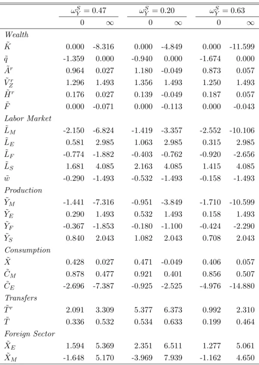
Panels (a) and (b) of Figure 3 show that the qualitative labor market and output effects are robust to changes inωYS. A larger informal sector (see the dotted lines) leads to a permanently larger fall in output and employment in both the manufacturing and aggregate market sector. The decline in the wage rate is less pronounced in the short run if the informal sector is large, because formal labor supply then decreases by more. Accordingly, a larger informal sector temporarily dampens the increase in formal agricultural employment and output, and vice versa (see the dashed lines). The effect on long-run wages, however, is independent of the size of the informal sector. Since the rental rate of capital is fixed, the change in the long-run capital-labor ratio in the import-competing sector—and associated with it the change in the steady-state wage rate—is fully determined by the change in the import tariff rate. Accordingly, the increases in both formal and informal agricultural employment and output in the long run are not affected by the size of the informal sector.
The import tariff cut lowers the relative price of the imported consumption good, so that consumption of the manufactured good increases both in the short and long run. Informal goods consumption also goes up, because the higher consumption tax rate induces households to substitute informal goods for formal agricultural goods. The time profile of full consump-tion is negatively sloped (see below), so that consumpconsump-tion of both formal goods decreases over time. However, consumption of the informal good increases during the transition, owing to expanding home production as workers are leaving the import-substitution sector. A larger informal sector amplifies the decrease in the consumption of formal agricultural goods, as more labor is relocated to production of informal agricultural goods.
4.2.2 Government Revenue
The tax-tariff reform leads to an increase in government revenue, in the short run as well as the long run [Panel (a) of Figure 3]. Although tariff revenue goes down on impact, this is more than offset by an increase in consumption tax revenue, owing to a larger consumption tax base (which includes both domestic and imported goods). In the long run, both the consumption tax and the import tariff generate more revenue than before the reform. Import tariff revenue increases, reflecting a positive tariff base effect that dominates the negative tariff rate effect in the long run. The base of the import tariff expands as the country imports more consumption goods. Intuitively, manufacturing output falls, whereas consumption of
Figure 3: Transitional Dynamics of a Tax-Tariff Reform Panel (a): : Labor Market and Public Revenue
˜ LF(t) L˜M(t) 0 20 40 60 80 100 120 140 160 180 200 −0.03 −0.025 −0.02 −0.015 −0.01 −0.005 0 time LF 0 20 40 60 80 100 120 140 160 180 200 −0.11 −0.1 −0.09 −0.08 −0.07 −0.06 −0.05 −0.04 −0.03 −0.02 −0.01 time LM ˜ LE(t) L˜S(t) 0 20 40 60 80 100 120 140 160 180 200 0 0.005 0.01 0.015 0.02 0.025 0.03 time LE 0 20 40 60 80 100 120 140 160 180 200 0.01 0.015 0.02 0.025 0.03 0.035 0.04 0.045 time LS ˜ w(t) T˜(t) 0 20 40 60 80 100 120 140 160 180 200 −0.015 −0.01 −0.005 0 time w 0 20 40 60 80 100 120 140 160 180 200 1 2 3 4 5 6 7 8x 10 −3 time T
Notes: The dashed line denotes the scenario ofωSY = 0.20, the solid line representsωYS= 0.47, and the dotted line depicts
Panel (b): Consumption and Output ˜ C(t) = ˜X(t) C˜M(t) 0 20 40 60 80 100 120 140 160 180 200 −1 0 1 2 3 4 5x 10 −3 time C 0 20 40 60 80 100 120 140 160 180 200 4 5 6 7 8 9 10x 10 −3 time CM ˜ CE(t) C˜S(t) = ˜YS(t) 0 20 40 60 80 100 120 140 160 180 200 −0.18 −0.16 −0.14 −0.12 −0.1 −0.08 −0.06 −0.04 −0.02 0 time CE 0 20 40 60 80 100 120 140 160 180 200 0.006 0.008 0.01 0.012 0.014 0.016 0.018 0.02 0.022 time CS ˜ YM(t) Y˜E(t) 0 20 40 60 80 100 120 140 160 180 200 −0.12 −0.1 −0.08 −0.06 −0.04 −0.02 0 time YM 0 20 40 60 80 100 120 140 160 180 200 0 0.005 0.01 0.015 time YE
Notes: The dashed line denotes the scenario ofωS
Y = 0.20, the solid line representsωYS= 0.47, and the dotted line depicts
ωS
Panel (c): Financial Assets and Wealth ˜ q(t) K(t)˜ 0 20 40 60 80 100 120 140 160 180 200 −18 −16 −14 −12 −10 −8 −6 −4 −2 0 2x 10 −3 time q 0 20 40 60 80 100 120 140 160 180 200 −0.12 −0.1 −0.08 −0.06 −0.04 −0.02 0 time K ˜ Vr Z(t) F˜(t) 0 20 40 60 80 100 120 140 160 180 200 0.0125 0.013 0.0135 0.014 0.0145 0.015 0.0155 time VZ 0 20 40 60 80 100 120 140 160 180 200 −1.5 −1 −0.5 0 0.5 1 1.5 2x 10 −3 time F ˜ Ar(t) H˜r(t) 0 20 40 60 80 100 120 140 160 180 200 −2 0 2 4 6 8 10x 10 −3 time A 0 20 40 60 80 100 120 140 160 180 200 −5 0 5 10 15 20x 10 −4 time H
Notes: The dashed line denotes the scenario ofωS
Y = 0.20, the solid line representsωYS= 0.47, and the dotted line depicts S
manufactured goods expands. The increase in public revenue depends negatively on the informal sector size, through its effect on the consumption tax base.
4.2.3 Financial Assets and Human Wealth
Panel (c) of Figure 3 shows that the net impact effect on financial wealth is positive. The positive jump in the value of land dominates the fall in Tobin’s q, because the employment share of the export sector compared to that of the import-substitution sector and the ad-justment speed of the investment system are large enough. Full consumption also jumps up, implying that the negative effect of the lower future physical capital stock is not strong enough to outweigh the immediate increase in financial wealth and the positive static effect on the return to human capital. The time profiles of financial wealth and full consumption are downward sloping, owing to a rising population share of new generations, who did not benefit from the increase in financial wealth at the time of the policy reform. Table 3 reveals that financial assets and human capital change in the long run by the same amount, which equals the change in full consumption [see (12)].
The jumps in financial wealth and full consumption are decreasing in the informal sector size, because a larger informal sector amplifies the fall in Tobin’sq and dampens the initial increase in the value of land. In the long run, however, the increase in both financial wealth and full consumption rises with the size of the informal sector. The reason is that a larger informal sector increases the importance of income from home production for human capital, which positively affects the long-run change in human capital. Panel (c) of Figure 3 shows that the long-run effects on full consumption, financial wealth, and human capital become negative if the informal sector is relatively small. In terms of Panel (b) of Figure 1, theA˙˜= 0 locus shifts down beyond its initial steady-state position.
The current account of the balance of payments turns into surplus in the short run— reflecting an immediate fall in investment—so that net foreign assets start to accumulate. At the same time, however, imports of manufactured goods rise by more than exports of formal agricultural goods. In the medium run, when the level of investment has settled down at its new equilibrium value, a deficit on the trade account materializes, so that net foreign assets go down and even become negative. The stock of net foreign assets thus display a non-monotonic adjustment path. In the new steady state, the current account is balanced again (i.e.,F˙˜(∞) = 0), implying that the interest payments on foreign debt need to be compensated by a trade account surplus. A larger informal sector positively affects the increase in exports by amplifying the fall in domestic consumption of the formal agricultural good, so that the decline in steady-state net foreign assets becomes smaller.
Table 3: Short-Run and Long-Run Allocation Effects (in Percent) ωSY = 0.47 ωYS = 0.20 ωYS = 0.63 0 ∞ 0 ∞ 0 ∞ Wealth ˜ K 0.000 -8.316 0.000 -4.849 0.000 -11.599 ˜ q -1.359 0.000 -0.940 0.000 -1.674 0.000 ˜ Ar 0.964 0.027 1.180 -0.049 0.873 0.057 ˜ VZr 1.296 1.493 1.356 1.493 1.250 1.493 ˜ Hr 0.176 0.027 0.139 -0.049 0.187 0.057 ˜ F 0.000 -0.071 0.000 -0.113 0.000 -0.043 Labor Market ˜ LM -2.150 -6.824 -1.419 -3.357 -2.552 -10.106 ˜ LE 0.581 2.985 1.063 2.985 0.315 2.985 ˜ LF -0.774 -1.882 -0.403 -0.762 -0.920 -2.656 ˜ LS 1.681 4.085 2.163 4.085 1.415 4.085 ˜ w -0.290 -1.493 -0.532 -1.493 -0.158 -1.493 Production ˜ YM -1.441 -7.316 -0.951 -3.849 -1.710 -10.599 ˜ YE 0.290 1.493 0.532 1.493 0.158 1.493 ˜ YF -0.367 -1.853 -0.180 -1.100 -0.424 -2.290 ˜ YS 0.840 2.043 1.082 2.043 0.708 2.043 Consumption ˜ X 0.428 0.027 0.471 -0.049 0.406 0.057 ˜ CM 0.878 0.477 0.921 0.401 0.856 0.507 ˜ CE -2.696 -7.387 -0.925 -2.525 -4.976 -14.880 Transfers ˜ Tr 2.091 3.309 5.377 6.373 0.992 2.310 ˜ T 0.336 0.532 0.534 0.633 0.199 0.464 Foreign Sector ˜ XE 1.594 5.369 2.351 6.511 1.277 5.061 ˜ XM -1.648 5.170 -3.969 7.939 -1.162 4.650
Notes: The parameters are set at their benchmark values in the first column. In the second
and third column, ΩS is changed to 0.60 and 0.95, implying ωS
Y = 0.20 andωYS = 0.63, respectively. The policy shock consists of ˜τM =−0.01 and ˜tC=−ετ˜M. To facilitate a sound comparison between the scenarios, variables with an ‘r’ in the superscript are scaled by their relative steady-state values instead of byY.
5
Welfare Effects of Tax-Tariff Reform
This section investigates the welfare effects of a consumer price-neutral tax-tariff reform start-ing from a calibrated initial equilibrium. Changes in the import tariff rate and the consump-tion tax rate have both efficiency and intergeneraconsump-tional welfare effects. To separate these two effects, we first discuss the special case of infinite planning horizons of households, so that only the pure efficiency effect is present. Subsequently, we analyze the effects on the intergenerational welfare distribution using the finite-horizon model.
5.1 Efficiency Effects
5.1.1 Command Outcome versus Decentralized Market Outcome
We first look at the infinite-horizon model (i.e., β = 0) as a special case. In this case, the model only features a steady state if the ‘knife-edge’ condition r = ρ holds. The first-best outcome follows from a command economy in which a social planner can allocate resources directly. The social planner’s optimization problem yields the following optimality conditions:
ε 1−ε CA(t) CM(t) = 1, (39) (1−αS)ΩSLS(t)−αS = (1−αM)ΩM K(t) LM(t) αM = (1−αE)ΩE ZE LE(t) αE , (40) ˙ q(t) +αMYKM((tt)) q(t) =r+δ− Ψ I(t) K(t) − 1 q(t) I(t) K(t) . (41)
Let us first analyze the case without an informal sector (i.e., ΩS = 0), so that the first equality
of (40) drops out. Comparing (39)–(41) with (7), (7), (19), and (23)–(25) reveals that the decentralized market equilibrium only coincides with the social planner’s solution if τM = 0.
Intuitively, there are no externalities in the model so that the tariff rate is the only variable distorting agents’ decisions on consumption, production, and investment. Because of the tariff distortion, too much capital and labor is allocated to the manufacturing sector and too little of the manufactured good is consumed domestically. The consumption tax is allowed to take on any value, because it does not distort the allocation of consumption across agricultural goods and manufactured goods. Therefore, starting from a positive pre-existing import tariff rate, the consumer price-neutral tax-tariff reform always improves welfare.
If an informal sector is present (i.e., ΩS > 0), then the first equality on the left-hand
side of (40) also holds. Consequently, the consumption tax is no longer irrelevant for welfare purposes, because it then distorts the allocation of labor between the formal and informal sector. The decentralized market economy now only coincides with the planner’s solution if
tC =τM = 0. Starting from positive pre-existing consumption tax and tariff rates, the
Figure 4: Welfare Effects of a Tax-Tariff Reform under Infinite Horizons: Plausible Cases
Notes: The pre-existing tax and tariff rates are: τM = 0.20, tC = 0.125 (solid line), tC = 0.175 (dotted line), and
tC= 0.225 (gray line). The policy shock consists of ˜τM =−0.01 and ˜tC=−ετ˜M.
the consumption tax distortion. Hence, the sign of the welfare change depends on the relative magnitudes of these two effects.
5.1.2 Welfare Results
By log-linearizing (1), while using (7) and (10), we obtain the change in lifetime indirect utility:23 dΛ∗RA(t) = X˜RA(t) ρ − Z ∞ t ˜ pC(z)e−ρ(z−t)dz = ˜ XRA(t) ρ , (42)
where we use the subscript RA to distinguish variables in the infinite planning horizon case from their counterparts in the overlapping generations formulation. The size of the informal sector has two opposing effects on the welfare change induced by the tax reform: (i) the consumption tax distortion increases (yielding a negative effect); and (ii) the tariff distortion gets smaller (yielding a positive effect). If the pre-existing consumption tax distortion is large compared to the pre-existing import tariff distortion, the negative effect dominates the positive effect so that a larger informal sector negatively influences the change in welfare. Conversely, if the pre-existing import tariff distortion is large compared to the pre-existing consumption tax distortion, the positive effect on the welfare change exceeds the negative effect for a specific range of informal sector sizes.
Figure 4 studies the effect of the informal sector size on the welfare change by varying the initial consumption tax rate. The welfare change is a monotonically negative function of the informal sector size if the initial consumption tax rate is high, whereas the relationship
23
The term capturing the price effect on lifetime welfare drops out, reflecting the price-neutrality of the tax-tariff reform.
Figure 5: Welfare Effects of a Tax-Tariff Reform under Infinite Horizons: Extreme Cases
Panel (a): VariousτM values andtC= 0.20 Panel (b): VarioustCvalues andτM = 0.15
Notes: In Panel (a), the pre-existing tax and tariff rates are: tC= 0.20,τM = 0.05 (solid line),τM = 0.10 (dotted
line), τM = 0.15 (gray line). In Panel (b), the pre-existing tax and tariff rates are: τM = 0.15,tC = 0.20 (solid line),tC= 0.30 (dotted line), andtC= 0.40 (gray line). The policy shock consists of ˜τM =−0.01 and ˜tC=−ετ˜M.
is non-monotonous if the initial consumption tax is low. On the upward-sloping part of the schedule, the fall in the tariff rate distortion dominates the rise in the consumption tax distortion, whereas on the downward-sloping part the rise in the consumption tax distortion is dominant. Although the pure efficiency effect may thus be decreasing in the size of the informal sector, it remains positive for all empirically plausible pre-existing tax and tariff rates. Figure 5 depicts two unrealistic parameter settings, in which case the welfare effect does become negative. In Panel (a), we choose a rather high consumption tax rate (i.e.,
tC = 0.20) and vary the import tariff rate between 0.05 and 0.15. In Panel (b), we set an
unrealistically low import tariff rate (i.e., τM = 0.05) and pick values of the consumption tax
rate in the range 0.10 and 0.30. Hence, only the combination of an unrealistically low import tariff rate and a rather high consumption tax rate (assuming ΩS > 0) renders the welfare
effect negative.
Our welfare findings for plausible conditions differ qualitatively from the results derived in a static model with an informal sector (cf. Emran and Stiglitz, 2005), because we take into account the distortionary effect of import tariffs on the investment decision of firms. As a result, a reduction in the import tariff rate is more beneficial in a dynamic model than in a static constellation.
5.2 Intergenerational Distribution Effects
We now turn to the model with a positive birth rate (i.e., β > 0), where we have to take into account that generations differ in the amount of wealth they have accumulated and therefore are affected differently by the reform. We distinguish between existing generations (represented by generation index v < 0) and future generations (represented by generation indexv=t≥0), where the time at which the policy reform takes place is normalized tot= 0. The welfare effect for existing generations is defined as the change in expected lifetime utility at the time of the reformdΛ∗(v,0), whereas the welfare effect for future generations is defined as the change in expected lifetime utility evaluated at birthdΛ∗(t, t). By log-linearizing (1), using (7) and (10), we find the change in lifetime utility for all generations (Appendix A.4):
dΛ∗(v, t) = ˜
X(v, t)
ρ+β . (43)
5.2.1 Existing Generations
Existing generations are born before the implementation of the policy shock and thus have al-ready accumulated financial assets. Equation (12) shows that full consumption is a fixed frac-tion of total wealth. Following Bovenberg (1993), the average welfare effect of the generafrac-tions currently alive is given by:
(ρ+β)dΛ∗(0) = 1− β β+r−ρ ˜ A(0) ωA + β β+r−ρ ˜ H(0) ωH , (44)
whereωH ≡rH/Y. Hence, the average welfare effect is a weighted average of the change in
financial wealth and human capital of existing generations. The coordinated tax-tariff reform boosts financial wealth at the time of the policy change, because the increase in the value of land—due to a current and future reallocation of labor to the export sector—dominates the negative wealth effect of the fall in Tobin’s q. Human capital is positively affected by an expansion of the informal sector—via the implicit income of informal workers—and a rise in lump-sum transfers and negatively by the drop in the wage bill of formal workers. In the benchmark scenario, human capital increases, reflecting the dominant effect of an increase in home production and lump-sum transfers. For plausible parameter values, the average welfare effect for the existing generations is positive as well.
Under the assumption that every existing generation has the same relative shares of equity and land in its portfolio, the welfare change for generationv is given by:
(ρ+β)dΛ∗(v,0) = 1−e(r−ρ)v A˜(0) ωA +e(r−ρ)vH˜(0) ωH , (45)
where 0 < e(r−ρ)v < 1 is the share of human wealth in the household’s wealth portfolio,
which is decreasing in the generation’s age. For relevant parameters, we find that the reform increases both short-run financial wealth and human capital, where financial wea