THE RESEARCH INSTITUTE OF INDUSTRIAL ECONOMICS
Working Paper No. 575, 2002
Discounting and Future Selves
by María Sáez-Martí and Jörgen W. Weibull
IUI, The Research Institute of Industrial Economics P.O. Box 5501
SE-114 85 Stockholm Sweden
Discounting and Future Selves
Maria Saez-Marti
∗Research Institute of Industrial Economics, Stockholm
Jörgen W. Weibull
†Stockholm School of Economics, and
Research Institute of Industrial Economics
21February 2002
Abstract
Is discounting of future instantaneous utilities consistent with altruism towards future selves? More precisely, can temporal preferences, expressed as a sum of dis-counted instantaneous utilities, be derived from a representation in the form of a sum of discounted total utilities? We find that a representation in the quasi-exponential (β, δ)-form in Phelps and Pollak(1968) and Laibson (1997) corresponds
to exponential altruism towards one’s future selves: the current self gives quasi-exponentially declining weights to her total utilities in future periods. For β = 1/2,
these welfare weights are exponential, while for β < 1/2 they are biased in favor of
the current self, and for β > 1/2 in favor of the future selves. More generally, we
establish a functional equation which relates welfare weights to instantaneous-utility weights and apply this equation to a number of examples. We also postulate five desiderata for instantaneous-utility discounting. None of the usual discount func-tions satisfy all desiderata, but we propose a simple class of discount funcfunc-tions which does.
JEL codes: D11, D64, D91, E21.
Keywords: Altruism, discounting, dynamic inconsistency, welfare.
∗This is a revised version of IUI Working Paper No. 572, 2002, “Welfare foundations of discounting.” The authors thank Philippe Aghion, David Laibson, Anders Martin-Löf, Arthur Robson, Ariel Rubinstein, Jean Tirole and Fabrizio Zilibotti for helpful comments and suggestions. A special thank to Ulf Persson who proved and generalized one of our conjectures. Saez-Marti thanks Vetenskapsrådet for financial support of her research.
†Weibull thanks the Laboratoire d‘Econométrie, Ecole Polytechnique, Paris, for its hospitality during part of his research.
1 Introduction
Samuelson (1937) introduced discounting of instantaneous utilities as a modelling approach in economics: “During any specified period of time, the individual behaves so as to max-imize the sum of all future utilities, they being reduced to comparable magnitudes by suitable time discounting.” (op. cit. p. 156). In order to obtain analytical tractability, he apologetically added the assumption that the discounting be exponential: “For simplicity we assume ... that the rate of discount of future utilities is a constant.... The arbitrariness of these assumptions is again stressed ...” (op. cit. p. 156).
Time preferences have recently come back into the foreground in the economics liter-ature, this time focusing on quasi-exponential or “hyperbolic” discounting, see Laibson (1997), Barro (1999), Krusell and Smith (1999) and Laibson and Harris (2001). Such pref-erences easily give rise to dynamic inconsistency.1 This implication from non-exponential
discounting was noted already by Ramsey (1928) and analyzed by Strotz (1956), Pollak (1968), Phelps and Pollak (1968), and Peleg and Yaari (1973).
In all these studies, preferences are represented by utility functions in the form of a sum of discounted instantaneous utilities. We here pose the question whether such preferences are consistent with the assumption of forward-looking agents who care about their future total utility, not only about their future instantaneous utilities. In other words: is discounting of future instantaneous utilities consistent with altruism towards future selves?2
Consider a decision-maker who is to choose a sequence x = (x0, x1, x2, ...) of
consump-tion vectors xt to b e consumed at dates t = 0, 1, 2, .... In Phelps and Pollak (1968) and
Laibson (1997), the consumer’s preferences at any decision time τ are represented by a
utility function of the form
Uτ(x) = u (xτ) + β ∞ t=1 δtu (x τ+t) , (1)
where β > 0 and 0 < δ < 1. The term u (xt) is interpreted as the instantaneous utility
in period t. We will call discount functions in the above (β, δ)-form quasi-exponential
(sometimes these are called quasi-hyperbolic), with exponential discounting as the special caseβ = 1.
In the cited studies, the function Uτ is decision theoretic in the usual sense of revealed
preferences: it determines the actual choice made by the consumer in period τ (with
1Dynamic inconsistency may arise if preferences are as in equation (1) below, and ifβ = 1: A sequence
x∗ = (x∗
0, x∗1, x∗2, ...) which maximizes U0 need not maximize Uτ for some τ > 0, given the “history”
x∗
0, x∗1, x∗2, ..., x∗τ−1 preceding period τ. The reason is simple: once a future period τ has become the present, the rate of substitution between the instantaneous utilities in periods τ + 1 and τ has changed
from its original valueδto the new valueβδ.
2An early discussion of the notion of “future selves”is Elster (1979).
due regard to the presence or absence of commitment possibilities). From a normative
viewpoint, Uτ(x) represents the welfare of the individual in period τ: the higher this
function value is, the “better off” is the individual in that period. Current welfare or “total utility”, so defined, does not stem only from current instantaneous utility but also from (the anticipation of) the stream of future instantaneous utilities. But, by assumption, this is true for the welfare in all future periods as well. In particular, the welfare in a future decision period τ > τ will in part depend on the instantaneous utilities in periods
t > τ. However, formula (1) does not explicitly account for future welfare. For example,
a marginal increase in instantaneous utility two periods ahead from some decision period
τ by an infinitesimal amount ε > 0 will add βδ2εu(x
τ+2) to current welfare, but it will
also add βδεu(x
τ+2)to welfare in the next period - an effect not explicitly accounted for
in equation (1).
We argue that a rational and forward-looking decision maker should respect the pref-erences of his or her future selves.3 In particular, if also future selves are forward-looking,
then this should not be neglected by the current self. Alternatively phrased: a rational decision maker who cares about his or her own welfare in future periods should strive to maximize some increasing function of her welfare in those periods. By contrast, an indi-vidual who in each period strives to maximize Uτ, as defined in equation (1), appears to
suffer from second-order myopia: she cares today about her future instantaneous utilities, but not about her future total utility (which also includes caring about her future total utility etc.).4 Does this matter for the induced behavior? Or are preferences of the form
(1) behaviorally equivalent with preferences that care about one’s future welfare?
In order to answer these questions we generalize formula (1) and study utility functions which can be written as a weighted sum of instantaneous utilities, and show that such functions have a welfare-theoretic foundation if the discount factor between successive periods is non-decreasing over time - as it indeed is in quasi-exponential and hyperbolic discounting. In particular, we find that a instantaneous-utility-based representation (1) in the “classical” exponential form, that is with β = 1, corresponds to one-period altruism:
the individual attaches weight δ to her welfare in the next period and weight zero to all
later periods (but her next self attaches weight δ to the welfare two periods ahead, etc. in
an infinite chain). Such preferences are sometimes assumed in intergenerational (dynastic) macroeconomic models, see for example Barro (1974) and Barro and Becker (1988).
We also find that instantaneous-utility-based representations (1) in the quasi-exponential form, that is with β < 1, correspond to quasi-exponential altruism towards one’s future
selves. The case β = 1/2 plays a special role. For such instantaneous-utility weights,
the welfare weights are in fact exponential; such individuals attach exponentially declin-3In the same vein, Lindbeck and Weibull (1988) analyze a simultaneous-move game between two altru-istic players who respect each others’ mutual altruism.
4A decision maker could be said to be first-order myopic if she does not even care about her future instantaneous utility from consumption, that is, if βδ = 0in eq. (1).
ing weight to their welfare in all future periods. For β < 1/2, the welfare weights are
quasi-exponential with a bias in favor of the current self (“myopia”), while for β > 1/2the
welfare weights are biased in favor of one’s future selves (“farsightedness”).
Another finding is that exponential welfare weights attached to the next T periods
-and weight zero to all future periods - yield instantaneous-utility weights that are based on the so-called Fibonacci sequence when T = 2, and forT > 2 on generalized Fibonacci
sequences.5 Moreover, we show that these instantaneous-utility weights need not decrease
monotonically over time. Indeed, such an individual may attach more weight to his in-stantaneous utility two periods ahead than to his inin-stantaneous utility next period. We also show, by way of examples, that certain instantaneous-utility-based preferences imply “spite” rather than “altruism” towards one’s future selves, i.e., a preference for as low as possible welfare in certain future periods. For example, if the parameterβ in equation (1)
would apply to periods t = 2, 3, ..., rather than to periods t = 1, 2, ..., then the associated
welfare weight two periods ahead would be negative.
To the best of our knowledge, we are the first to identify the recursive functional equation that constitutes the link between discounting of instantaneous utilities and total utilities. However, already Zeckhauser and Fels (1968) started from a certain welfare rep-resentation based on total utilities, and derived the corresponding reprep-resentation based on instantaneous utilities.6 Their main result was that “perfect altruism”, that is,
exponen-tial discounting of instantaneous utilities, is incompatible with their chosen representation based on total utilities.7 As indicated above, however, this claim is not valid in our
frame-work; the welfare representation of exponential discounting of instantaneous utilities is the above-mentioned one-period altruism (see section 3.1 below).
The present investigation may also have some bearing on a related modelling issue in macroeconomics, namely whether it matters, in models of sequences of altruistic gen-erations, if each generation cares only about the next generation’s instantaneous or total utility, or about all generations’ instantaneous or total utility, see for example Barro (1974), Andreoni (1989) and Abel and Bernheim (1991).
The remainder of the paper is organized as follows. Section 2 provides the model, and section 3 establishes a one-to-one relationship between welfare weights and instantaneous-utility weights. Section 4 analyzes a few examples from the literature, and section 5 5The Fibonacci sequence is 1, 1, 2, 3, 5, 8, 13, ...., each term, after the first two, being the sum of the two preceding terms.
6In our notation, their welfare representation was
Uτ(x) = u (xτ) + bUτ(x) + d ∞ t=1 atU τ+t(x)
7More exactly, they found that this implies b = 1, which makes their welfare representation undeter-mined, see previous footnote.
postulates some desiderata for discounting functions. None of the usual formulations satisfy all desiderata, but in section 6 we propose a simple parametric family of discount functions which meet the desiderata. Section 7 concludes. Mathematical proofs are collected in an appendix at the end of the paper.
2 The model
Consider an infinitely lived individual who makes decisions over a sequence of periods
t ∈ N = {0, 1, 2, ...}. In each periodt, the individual consumes some vectorxt ∈ X, where
X ⊂ Rnis a set of consumption alternatives andn ∈ N
+ = {1, 2, ...}. Aconsumption stream
x is an infinite sequence of consumption vectors xt, and we write x = (x0, x1, ...) ∈ X∞.8
Let τbe the preferences of the decision maker in period τ over consumption streams
x ∈ X∞. A preference profile for the individual is a sequence (
τ)τ∈N of preferences,
one for each “self τ”.
We here study preference profiles that can be represented by stationary and additively separable utility functions of the type used in the macroeconomics literature. More exactly, we focus on preference profilesττ∈N for which there exists functionsUτ : X∞ → R, one
for each decision period τ ∈ N, such that x τ y if and only if Uτ(x) ≥ Uτ(y), where
Uτ(x) = ∞
t=0
f(t)u (xτ+t) (2)
for some u : X → R+ and f : N → R+ with the normalization f (0) = 1. Here u (xs) will
be called the instantaneous (sub)utility from consumption in period s, andf(t)theweight
that the decision maker assigns to her instantaneous utility t periods later.
We will say that a sequenceUττ∈N of such utility functions admits a (stationary and
additively separable) welfare representation if for all τ ∈ Nand x ∈ X∞,
Uτ(x) = u (xτ) + ∞ t=1 f∗(t) U τ+t(x) , (3) for some f∗ : N
+ → R. Here f∗(t) is the weight that the decision maker places on her
welfare or total utility t periods later.
A negative weight attached to another individual’s welfare expresses “spite” rather
than “altruism.” Such welfare weights appear pathological in the present context.9 We
will hence call a welfare-weight function f∗ regular if it is non-negative. In this case we
will say that Uττ∈N admits a regular welfare representation. 8Of course,x
tneed not be consumption.
9We do not deny that the excluded possibility may sometimes be psychologically relevant, but it appears not to be typical for consumers in conventional decision problems.
3 The welfare representation
Does the sequence Uττ∈N defined in equation (1) admit a regular welfare representation?
If so, which? A key result for answering this and related questions is the observation that every sequenceUττ∈N in the more general form (2) admits a welfare representation of the
form (3), and, moreover, f∗ : N
+ → R is uniquely determined by the following system of
recursive equations:
f∗(t) =
f (1) if t = 1
f(t) −t−1s=1f(t − s)f∗(s) if t > 1 . (4)
Proposition 1: If Uτ satisfies equation (2) for some u : X → R and f :
N → R, then Uτ admits the welfare representation (3), where f∗ : N+ → R
is the unique solution to (4).
(See Appendix for a proof.)
Conversely, the instantaneous-utility weight function f may be obtained from the
welfare-weight function f∗ via equation (4), which implies
f(t) =
f∗(1) if t = 1
t−1
s=0f∗(t − s)f(s) if t > 1 , (5)
a recursive equation system which uniquely determines f fromf∗ (recall the normalization
f (0) = 1). This equation states that the instantaneous-utility weightf(t)can be computed
as the sum of that period’s instantaneous utility’s contributions to the decision maker’s welfare in all interim periods.
It is immediate from equation (5) that if f∗ is non-negative, so is f. However,
Propo-sition 1 does not claim that the welfare representation necessarily be regular, even if f
is non-negative. Indeed, the welfare-weight function f∗ may well take negative values
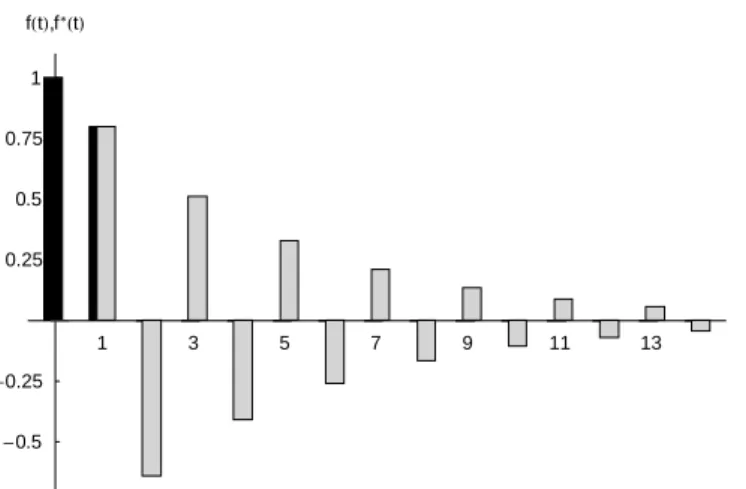
although all instantaneous-utility weights are positive. To see this, note that (4) gives
f∗(2) = f (2) − f2(1). Hence, in order for the welfare weight f∗(2) to be negative it
suffices that f (2) < f2(1). This is the case, of course, if f (1) > 0 but f (2) = 0.10 The
welfare representation is non-regular, see Figure 1 below.11
Another example is whenf is of the hyperbolic form f(t) = 1/ (0.5 + t); thenf2(1) =
(2.25)−1 > f (2) = (2.5)−1. A third example is f(t) = 1/ (1 + t2), yielding f2(1) = 1/4 >
f(2) = 1/5. A fourth example is when the β in the quasi-exponential representation (1)
kicks in with one period’s delay, that is, when f (1) = δ and f (2) = βδ2 for someβ < 1. 10This arises as a special case of the preference structure in the intergenerational analyses in Lane and Mitra (1981) and Leininger (1986), where each generation’s welfare is as a function of its own consumption and that of its immediate descendant.
11It is easy to verify that equation (4) givesf∗(t) = (−1)t+1f (1)t. 6
1 3 5 7 9 11 13 t -0.5 -0.25 0.25 0.5 0.75 1 fHtL,f*HtL
Figure 1: Instantaneous-utility weights f(1) = δ and f(t) = 0 for t > 1 (black bars), for δ = 0.8, and the corresponding welfare weights,f∗(t) (gray bars).
Then clearly f∗(2) = f(2)−f2(1) = (β−1)δ2 > 0.12 See Figure 2 below. In all four
cases, the decision-maker is constantly spiteful to his future self two periods ahead.
1 3 5 7 9 11 13 t -0.25 0.25 0.5 0.75 1 fHtL,f*HtL
Figure 2: Instantaneous-utility weights f(1) =δ and f(t) = βδt for t >1 (black bars), for
δ = 0.8 andβ = 0.6, and the corresponding welfare weights,f∗(t) (gray bars).
A sufficient condition for all welfare weights to be non-negative, and hence for the welfare representation to be regular, is that all instantaneous-utility weights are positive and that the ratio between successive instantaneous-utility weights - the discount factor between successive periods - be non-decreasing over time. Equivalently, the discount rate should be non-increasing. Formally:
Proposition 2: Suppose f : N → R++ and let g : N+ → R be defined by
12This situation would arise if, say, the underlying continuous-time discounting function would beϕ (t) =
δt for t < 1 andϕ (t) = βδt for t ≥ 1, where t ∈ R
+. If the decision times aret = 0, 1, 2, 3, ..., then (1) applies, while if the decision times aret = 0,1
2, 1,32, ..then the discrete-time instantaneous-utility weights, sequentially labeled, would bef (0) = 1,f (1) = δ1/2,f (2) = βδ,f (3) = βδ3/2etc.
g(t) = f(t)/f(t−1). If g is non-decreasing, then f∗ ≥ 0. If g is strictly
increasing, then f∗ >0.
The proof of this result, based on our initial and more restrictive conjecture, was kindly provided by Ulf Persson (see appendix).
The discount functionf in the quasi-exponential form (1), for β,δ∈[0,1], clearly satisfy
this monotonicity condition; theng(1) =βδ ≤g(t) =δ for all t >1. Diamond and K˝oszegi
(Appendix D, 1999) study a “more hyperbolic” version of (1), namely where f(1) = βγδ
and f(t) = βγ2δt for all t > 1, for some β,γ,δ ∈ [0,1]. Also these discount functions
meet the monotonicity condition; then g(1) =βγδ ≤g(2) =γδ ≤ g(3) =g(4) =...=δ.
Hence, each of these representations has a regular welfare foundation.
As a more general comment, we note that with f,f∗ ≥ 0, we have 0 ≤ f∗(t) ≤ f(t)
for all positive integers, by (4). If, moreover, f(t)→0 ast → ∞, then so doesf∗(t).
In the following section we analyze examples of instantaneous-utility-based and welfare-based discount functions.
4 Examples
4.1 Exponential instantaneous-utility weights
Suppose the instantaneous-utility weights decline exponentially: f(t) = δt for all t, for
some δ ∈(0,1). This is the standard case in macroeconomic modelling, corresponding to
the special case β = 1 in equation (1). It is not difficult to verify that equation (4) then gives f∗(1) =δ and f∗(t) = 0 for all integers t >1.
To see this, first note that equation (4) gives f∗(1) =δ and f∗(2) = 0. Suppose that
f∗(1) =δ and f∗(s) = 0 for alls = 2,..,t−1. Then (4) gives
f∗(t) =δt−t−1 s=1δ
t−sf∗(s) =δt−δt−1δ= 0 . (6)
Hence, by induction this holds for all positive integers t.
Conversely, suppose that the decision maker cares only about her current instantaneous utility and her welfare in the next period. Then f∗(1) =α, for some α >0, andf∗(t) = 0
for all integers t >1. An application of equation (5) immediately gives f(t) =αt for allt.
Hence, the reduced form (2) for such an individual is indeed exponential: Uτ(x) = ∞ t=0 αtu(x τ+t) , (7)
where the discount factor equals the weight that the decision maker attaches to his or her welfare in the next period.
In sum: exponential instantaneous-utility weights have a regular welfare foundation. Zero weight is given to the welfare in all future periods beyond the next.
4.2 Exponential welfare weights
Suppose instead that it is the welfare weightsf∗(t)that decrease exponentially over future
periods t. What are then the associated instantaneous-utility weights? More exactly,
suppose thatf∗(t) = αtfor someα ∈(0,1) and for allt. Equation (5) then gives f(1) =α,
f(2) = 2α2, and f(3) = 4α3. One may thus conjecture that
f(t) = 12 (2α)t ∀t >0. (8)
This conjecture is easily proved to be true by induction, see appendix. Substituting (8) in (2) we thus obtain Uτ(x) =u(xτ) + 12 ∞ t=1 δ tu(x τ+t) , (9)
for δ = 2α. Hence, exponential altruism is equivalent to the Phelps-Pollak-Laibson repre-sentation (1) with β = 1/2.
Note that in the special case whenα = 1/2, we haveδ = 1and thus f(t) = 1/2 for all integers t. Hence, in this case the same weight is given to the instantaneous utility in all time periods. This special case is relevant from a biological viewpoint, since the genetic kinship between any pair of successive generations is precisely 1/2.
4.3 Finite-horizon exponential welfare weights
We next consider the intermediate cases between one-period altruism and exponential altruism, namely when the welfare weight decreases exponentially over a finite number of time periods, beyond which all weights are zero. What is the corresponding reduced form (2)?
More exactly, let T > 1, and suppose f∗(t) = αt for some α ∈ (0,1) and for all
t ≤ T, with f∗(t) = 0 for all t > T. It can then be verified that f can be written as
fT(t) =mT(t)αt, where
mT(t) =
min{t,T }
s=1 m
T(t−s) (10)
for all positive integers t, and mT(0) = 1(see appendix). It follows from (10) that, for any
finite horizon T,
1≤mT(t)≤mT+1(t)≤2t−1 (11)
and
αt ≤f
T(t)≤fT+1(t)≤ 12(2α)t (12)
for all t. Hence, the longer the altruism horizon T, the higher the weight given to each
future instantaneous utility.
Moreover, it follows from an established result for recursive equations that the ratio between the mT-weights assigned to two consecutive periodst and t+1converges ast goes
to infinity (see e.g. Weisstein, 1999), for any given T >1:
lim t→∞ fT(t+ 1) fT(t) =αt→∞lim mT(t+ 1) mT(t) =αλT , (13)
where λT is the unique solution λ > 1 of λ = 2− λ−T. Notice that λT is increasing
in T, and limT →∞λT = 2. Hence, for each T > 1, the instantaneous-utility weights are
asymptotically exponential with discount factorαλT.
In particular the sequencem2(t)is the Fibonacci sequence. The ratio between
succes-sive Fibonacci numbers is known to converge to the so-called golden number (Kelley and Peterson, 1991): m2(t+ 1) m2(t) →λ2 = 1 + √ 5 2 . (14)
Note also that the induced weight function,f, need not be monotonic. In fact, for all T ≥ 2 and α > 1/2: f(1) < f(2) < f(0). Figure 3 illustrates this feature for T = 2 and
α = 0.6 1 3 5 7 9 11 13 t 0.25 0.5 0.75 1 fHtL,f*HtL
Figure 3: Instantaneous-utility weights,f(t)(black bars), and welfare weights, f∗(t)(gray
bars), with two-period-horizon exponential altruism, with α= 0.6. 4.4 Quasi-exponential instantaneous-utility weights
We found that exponential welfare weights imply quasi-exponential instantaneous-utility
weights (β,δ) with β = 1/2. What welfare weights correspond to quasi-exponential
instantaneous-utility weights (β,δ) when β = 1/2? 10
Suppose, thus, thatf(0) = 1andf(t) =βδtfor all positive integers. Thenf∗(1) =βδ
and f∗(2) =β(1−β)δ2. It is not hard to prove by induction that
f∗(t) =β(1−β)t−1δt ∀t (15)
(see appendix). Hence, a representation in the Phelps-Pollak-Laibson form (1), withβ = 1, is the reduced form of a welfare representation (3) in the quasi-exponential form
Uτ(x) =u(xτ) +β∗ ∞ t=1 (δ∗)tU τ+t(x) , (16) where β∗ =β/(1−β) and δ∗ = (1−β)δ. (17)
Quasi-exponential instantaneous-utility weights thus do have a regular welfare founda-tion, namely quasi-exponential welfare weights. We note that the “welfare myopia” factor β∗ is an increasing function of the “instantaneous-utility myopia” factor β, such that β∗
reaches the value1 - hence exponential welfare weights - precisely when β reaches 1/2, an observation that is consistent with our earlier finding in the case of exponential welfare
weights. At β = 1/2, welfare weights switch from being biased toward “myopia” to being
biased toward “farsightedness.”
Angeletos et al (2001) made the following estimate of the parameter pair (β,δ) in
the Phelps-Pollak-Laibson model, based on annual US data: β = 0.55and δ = 0.96. The
associated welfare representation is thus slightly biased toward “farsightedness”: β∗ = 1.22
and δ∗ = 0.43. In other words, individuals place relatively more weight on their future
welfare, in comparison with exponential weights: f∗(1) =β∗δ∗ = 0.52, f∗(2) =β∗(δ∗)2 =
0.23etc.
4.5 Hyperbolic instantaneous-utility weights
Empirical studies of temporal preferences suggest that the discount function f be
hyper-bolic, rather than exponential. Hence, Ainslie (1992), following Herrnstein (1981) and Mazur (1987), suggests f(t) = (λ+µt)−1 for some λ,µ >0 (op. cit. eq. (3.7)). A similar
hyperbolic expression, (1 +µt)−β/µ is suggested by Loewenstein and Prelec (1992).
As noted above, for certainλ and µ, the first form may correspond to negative welfare weights - a non-regular welfare representation. In particular, such hyperbolic preferences
express spite against oneself two periods ahead (after each current period) if and only if
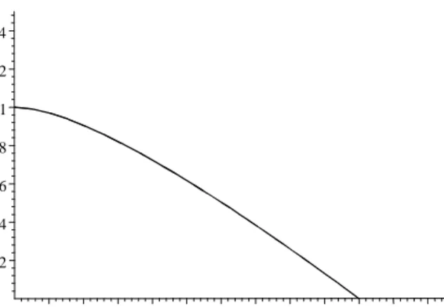
(λ+µ)2 < λ+ 2µ. In Figure 4 below, which has µ on the horizontal and λ on the vertical axis, this is the area below the curve.13
13Recall that f∗(2) = f (2) − f2(1). Also note that f∗(1) = f (1) ≤ 1 iff λ + µ ≥ 1.
0.2 0.4 0.6 0.8 1 1.2 1.4 0.2 0.4 0.6 0.8 1 1.2 1.4 1.6 1.8 2 2.2 2.4
Figure 4: Points below the curve are parameter combinations (µ,λ) for which the welfare
weightf∗(2) is negative.
Clearly, the sufficient condition for non-negative welfare weights in proposition 2 is violated if (λ+µ)2 < λ+ 2µ. However, it also turns out that all welfare weights are
non-negative when the inequality does not hold. Hence, the result in proposition 2 is sharp in
this special case. To see this, let f(0) = 1 and f(t) = (λ+µt)−1 for all positive t. Then
g(t+ 1)≥g(t)for allt if and only if g(1)≥g(0), which is equivalent to(λ+µ)2 ≥λ+2µ.
Without any loss of generality, we relabel the parameters in the second form mentioned above, and study
f(t) = (1 +at)−b ∀t ∈ N, (18)
for a,b > 0. It follows from proposition 2 that the corresponding welfare-weight function f∗ is everywhere positive, since f > 0 and the discount factor between successive periods
is strictly increasing over time:
g(t) = f(ft(−t)1) =1− 1 +aat b
. (19)
We do not have an explicit formula forf∗, though. Instead, using equation (4) we have
generated the welfare weights f∗(t), for t = 1,2,...,50, for different combinations of a and
b, and fitted the function
˜
f(t) = θ
(1−a˜+ ˜at)˜b (20)
to the data. (Note that f˜(1) =θ.)
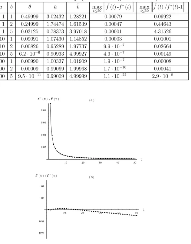
Table 1 reports the estimatesa,˜ ˜b and θ, as well as the maximum absolute and relative errors in the first50periods. We note that, for fixeda,a is decreasing and˜ ˜b increasing in b. Moreover, ˜a≈1and˜b≈b when a is large. Figure 5 below shows the welfare weights f∗(t)
(dots) obtained from equation (5), for a = 10 and b = 1, the estimated function-values
˜
f(t), as well as the ratio f˜(t)/f∗(t).
Table 1: Estimates of f∗ (obtained through Mathematica).
a b θ ˜a ˜b maxt≤50 f˜(t)-f∗(t) max t≤50 f˜(t)/f∗(t)-1 1 1 0.49999 3.02432 1.28221 0.00079 0.09922 1 2 0.24999 1.74474 1.61539 0.00047 0.44643 1 5 0.03125 0.78373 3.97018 0.00001 4.31526 10 1 0.09091 1.07430 1.14852 0.00003 0.01001 10 2 0.00826 0.95289 1.97737 9.9·10−7 0.02664 10 5 6.2·10−6 0.90933 4.99927 4.3·10−7 0.00149 100 1 0.00990 1.00327 1.01909 1.9·10−7 0.00008 100 2 0.00009 0.99069 1.99968 1.7·10−10 0.00041 100 5 9.5·10−11 0.99009 4.99999 1.1·10−22 2.9·10−8 10 20 30 40 50 t 0.96 0.98 1.02 1.04 fˆHtLêf∗HtL HbL 10 20 30 40 50 t 0.02 0.04 0.06 0.08 f∗HtL,fˆHtL HaL
Figure 5: (a) Welfare weights f∗(t) obtained from equation f(t) = (1 + 10t)−1 (dots) and
the estimated function f˜(t) (solid line). (b) The ratio f˜(t)/f∗(t).
5 Desiderata for stationary discount functions
Having examined circumstances under which utility functions Uτ in the form (2) have a
regular welfare foundation in the form (3), we now turn to a discussion of some other desiderata.
Our first desideratum is that the representation (2) should be invariant with respect to periodization, in the sense that there should exist a continuous-time discount function from which the discrete-time discount factor f(t)in each period t can be derived, for any given period length∆>0. The Phelps-Pollack-Laibson model (1), to be referred to as the
PPL model, is unclear in this respect, since it states that discounting kicks in from period
1 on, without specifying for what lengths ∆of the time period this should hold, or, more
generally, how the parameters β and δ should be adjusted if the time period is changed
(c.f. discussion and figure in section 3). In exponential discounting models one usually
assumes δ= exp(−r∆)for some real-time discount rate r, but what about β?
Secondly, empirical studies suggests that the considered class of discount functions should contain some form of hyperbolic discounting as a special case. As mentioned above, hyperbolic discounting of instantaneous utilities has been shown to fit the data better than exponential discounting. It therefore seems desirable that the considered class contain such hyperbolic discounting as a special case. Clearly the quasi-exponential PPL representa-tion does not meet this second desideratum exactly, only approximately over the first few periods.14
Third, exponential discounting has traditionally been the main approach in economics, and should therefore be contained in the class. The PPL representation clearly meets this desideratum (just set β = 1in equation (1)).
If a random variable T is exponentially distributed, then its conditional probability
distribution, given T ≥ t, is identical to the original, for any t. It is precisely this time
homogeneity property that guarantees dynamic consistency in intertemporal decision prob-lems. As a weaker requirement, in the present context of discount functions, our fourth desideratum is that the class of discount functions considered should be “closed under truncation” in the sense that the normalized discount factors, from any given future date on, should belong to the class. When currently contemplating a future decision point, in a dynamic decision problem, it should not be necessary to step outside the class. The PPL-representation evidently satisfies this desideratum: the decision maker’s preferences over future periods are exponential.
Finally, the discounting of instantaneous-utilities should have a regular welfare founda-tion. We saw above that the PPL representation (1) satisfies this last desideratum as long as β ≤1.
Formally, we consider preferences over infinite consumption streams x represented in
14The same is true for the “more hyperbolic” formulation in Diamond and K˝oszegi (1999).
the form Uτ(x) = ∞ t=0 ϕ(t,∆)u(x τ+t), (21)
where ϕ(t,∆)is the discount factor that the decision maker in periodτ ∈ Nassigns to his
or her instantaneous utility in period τ+t, if the length of each period is ∆>0.
LetF be any family of functions ϕ:N × R+ → R+ such thatϕ(0,∆) = 1for all∆>0.
Our desiderata are
D1(invariance w.r.t. periodization): There exists a function f : R+ → [0,1] such that ϕ(t,∆) =f(t∆) for all t∈ N and ∆>0.
D2(hyperbolic discounting allowed): Every function ϕ of the form ϕ(t,∆) = (1 +αt∆)−β, for some α,β >0 ,belongs to F.
D3(exponential discounting allowed): Every function ϕ of the form ϕ(t,∆) = exp(−γt∆) for some γ >0,belongs to F.
D4(algebraic closure under truncation): If ϕ∈ F,then also ϕτ ∈ F for any
τ ∈ N+, where ϕτ :N × R+ →[0,1] is defined by
ϕτ(t,∆) = ϕϕ(τ(+τ,∆)t,∆) ∀t ∈ N.
D5(regular welfare foundation): If ϕ ∈ F, and f : N →[0,1] is defined by
f(t) =ϕ(t,1) for all t,then the associated welfare weights f∗(t) are all
non-negative.
6 Hyperbolic-exponential discount functions
One family F which meets all desiderata are the functions ϕ of the form
ϕ(t,∆) = (1 +at∆)−be−ct∆ (22)
for some a,b,c > 0. This family F is three-dimensional, the minimal parametric
dimen-sionality for the PPL model to hold across different time discretization. Hence, we have not added any real degree of freedom above and beyond that of the PPL model.
It is not difficult to see that all five desiderata indeed hold. Desideratum 1 is given by construction. Also desiderata 2 and 3 are self-evident; one obtains exponential discounting
by setting b= 0, and hyperbolic discounting by setting c= 0. That desideratum 4 holds
follows from
ϕτ(t,∆) = (1 +at∆)−be−ct∆, (23)
where a = a/(1 + ∆τa) > 0. In other words, ϕ
τ ∈ F. Note that the parameters b and
c are unaffected by such truncation of the past, while the parameter a changes. Dynamic
inconsistency arises from the single fact that this parameter decreases with the number τ
of past periods, for any fixed period length ∆. To finally see that desideratum 5 holds,
note that:
f(t) =βtδt for allt ∈ N, (24)
where βt = (1 +at)−b and δ = e−c. Since the discount factor g(t) = δβt/βt−1 between
successive periods accordingly is strictly increasing, all welfare weights f∗(t) are positive
by proposition 2.
This family of discount functions is closely related to the PPL model. We here have β0 = 1, and g(t) =δβt+1/βt→δ as t→ ∞, just as in the PPL model.
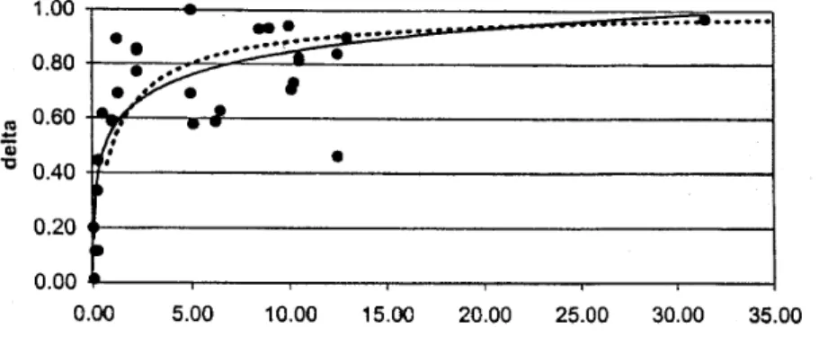
As a final remark, we note that the present family of discount functions seems to be sufficiently rich to fit a wide range of empirical observations. Frederick, Loewenstein and O’Donoghue (2001) report empirical estimates of discount rates from no less than 40 studies (Table 2, op. cit.) Their general finding is that the average discount rate over longer time intervals is lower than the average discount rate over shorter time intervals. Figure 6 below is their Figure 1, with the addition of the dotted curve. The points are their data points, and the solid curve has been fitted by them, while the dotted curve has been fitted by us,
from a discount function from the present family F.15 This fitting was made by way of
“eye econometrics,” resulting in the following estimates: a= 10, b= 0.3 andc= 0.16
Figure 6: Fitting a discount function f (dotted curve) from the family F to the data in
Figure 1 of Frederick, Loewenstein and O’Donoghue (2001).
Figures 7 and 8 compare the instantaneous-utility weightsf(t)and the welfare weights 15The dotted curv e is the graph of y (t) = [f (t)]1/t = (1 +at)−b/te−c, for a= 10, b= 0.3 and c = 0. Note that limt→0y(t) = exp[−(ab+c)] and limt→+∞y(t) = exp(−c).
16Hence, according to this rough estimate, there is no need for an exponential factor - hyperbolic dis-counting is sufficient. Needless to say, however, more careful empirical studies are needed for any general conclusion of this sort.
f∗(t)corresponding to our estimate,f(t) = (1+10t)−0.3 (grey bars), with the Laibson et al
(2001) estimate (black bars in figure 7) and with exponential discounting with an annual
discount rate of 5% (black bars in figure 8). The latter is the macro-based estimate of
Cooley and Prescott (1995).17
0 2 4 6 8 10 12 14 t 0.2 0.4 0.6 0.8 1 fHtL HaL 0 2 4 6 8 10 12 14 t 0.2 0.4 0.6 0.8 1 f* HtL HbL
Figure 7: (a)f(t) = (1+10t)−0.3 (gray) and quasi-exponential instantaneous-utility weights
(β,δ), for β = 0.55and δ= 0.96 (black). (b) The corresponding welfare weightsf∗(t).
0 2 4 6 8 10 12 14 t 0.2 0.4 0.6 0.8 1 fHtL HaL 0 2 4 6 8 10 12 14 t 0.2 0.4 0.6 0.8 1 f* HtL HbL
Figure 8: (a) f(t) = (1 + 10t)−0.3 (gray) andf(t) =e−0.05t (black). (b) The corresponding
welfare weights f∗(t).
7 Conclusion
We started out by asking if discounting of future instantaneous utilities is consistent with altruism towards future selves, within a stationary and additively separable modelling framework. We identified a recursive functional equation which relates welfare weights - the altruistic weight attached to the total utility of future selves - to the weights given to future
17To be more precise, they give the estimate 0.987 of the quarterly discount factor.
instantaneous utilities. If the welfare weights are non-negative, so are the instantaneous-utility weights. However, the converse is not true in general. Indeed, we saw that certain discounting schemes in the literature are inconsistent with altruism towards one’s future selves or towards future generations. We also established a sufficient condition for consis-tency in this respect, namely that the discount factor attached to instantaneous utilities between successive periods should not decrease over time. In other words, the discountrate
should be non-increasing. (Recall that this rate is constant under exponential discount-ing.) The quasi-exponential discounting models which are currently under investigation in the macroeconomics literature (see for example. Laibson (1997), Barro (1999), Krusell and Smith (1999), Laibson and Harris (2001) and Angeletos et al (2001)) all have this property, as do some of the hyperbolic discounting models in the psychology literature (see for example Herrnstein (1981), Mazur (1987) and Ainslie (1992)). Indeed, the property of a decreasing discount rate seems to conform with all available empirical data, both for humans and animals.
Moreover, estimates of the parameterβ in the Phelps-Pollak-Laibson (1) model suggest
β-values near0.5(Angeletos et al, 2001). In our theoretical investigation, we found thatβ = 0.5 corresponds to exponentially declining weights given to future selves (or generations).
Is this a mere coincidence or is there some more profound reason to expect β-values to be
near 0.5? Perhaps this question should not be taken too seriously, however, since empirical
estimates presumably depend in part on the periodization of the time-series data. An interesting question thus is whatβ-estimates one obtains for different period lengths. Such a study could also shed light on one of the five desiderata that we postulate at the end of the study: the discount function for instantaneous utilities should be consistent with some continuous-time discount function.18 More generally, we hope the present theoretical study
can be of some help when discriminating between different functional forms in subsequent empirical work on time preferences.
An important question that this study leaves open is the mathematical tractability of the proposed hyperbolic-exponential discounting functions when used in dynamic op-timization. Laibson and Harris (2001) were able to generalize the Euler equations from exponential to quasi-exponential discounting, which was not an easy task. It seems that the step from exponential to hyperbolic-exponential discounting is even bigger and may lead to involved first-order conditions.
From the viewpoint of experimental studies of intertemporal preferences, finally, all the discounting models discussed here seem quite restrictive. See, for example, Freder-ick, Loewenstein and O’Donoghue (2001) and Kahneman (2000), and see also Rubinstein (2001) for a critical discussion of discounting models. Hence, generalizations in behaviorally relevant directions are called for.
18The same requirement for the welfare weights does not seem to make sense, since in the limit as the period shrinks to zero, each self has zero life span.
8 Appendix
8.1 Proof of proposition 1
Suppose Uτ satisfies equation (2) for some u : X → R and f : N → R with f(0) = 1.
Let f∗ : N+ → R be defined by (4). Then
f(t) =t s=1 f∗(s)f(t−s) ∀t∈ N+ . Hence, Uτ(x) = u(xτ) + ∞ t=1 t s=1 f∗(s)f(t−s)u(x τ+t) = = u(xτ) + ∞ s=1 f∗(s) ∞ t=s f(t−s)u(xτ+t) = u(xτ) + ∞ s=1f ∗(s) ∞ k=0 f(k)u(xτ+s+k) =u(xτ) + ∞ s=1f ∗(s)U τ+s(x)
Since this holds for all τ, this proves the claim. 8.2 Proof of proposition 2
Suppose first that g is non-decreasing. We know that f∗(1) =f(1) >0. Suppose f∗(s) ≥
0 ∀s < t. Then f∗(t) = f(t) −f(1)f∗(t− 1) −t−2 s=1f ∗(s)f(t−s) = g(t)f(t− 1) −f(1)f∗(t− 1) −t−2 s=1 g(t−s)f∗(s)f(t−s− 1) ≥ g(t) f(t− 1) − t−2 s=1 f∗(s)f(t−s− 1) −f(1)f∗(t− 1) = g(t)f∗(t− 1) −f(1)f∗(t− 1) = [g(t) −f(1)]f∗(t− 1) ≥ 0.
The last inequality follows from the assumption that g is non-decreasing and f(1) =g(1).
Secondly, suppose that g is strictly increasing. Suppose f∗(s) > 0 ∀s ≤ t. The same
reasoning as above then leads to f∗(t)>[g(t) −g(1)]f∗(t− 1) >0.
8.3 Proof of equation (8)
Suppose f(s) = 2s−1αs fors = 1,2,..,t, for some positive integer t. Then (5) gives
f(t+ 1) = αt+1 +t s=1 2s−1αsαt+1−s =αt+1 1 + t s=1 2s−1 = αt+1 1 + (2t− 1)= 2tαt+1.
By induction in t, this establishes (8). 8.4 Proof of equation (15)
Equation (15) may be established by induction over t, as follows. First note that f(1) =
f∗(1). Suppose that equation (15) holds for all s < t for some t. Equation (5) then gives
f(t) = f∗(t) +t−1 s=1 f∗(s)f(t−s) = β∗(δ∗)t+t−1 s=1 β ∗(δ∗)s(δ∗/δ)sβδt = β∗(δ∗)t+βδt t−1 s=1β ∗(1 −β)s = β∗(δ∗)t+βδt1 − (1 −β)t−1 = βδt 8.5 Proof of equation (10) Under equation (10), we have
f(t) = αtmin {t,T } s=1 m(t−s) =αtmin {t,T } s=1 αs−tf(t−s) = min{t,T } s=1 αsf(t−s).
Setting f∗(s) =αs for all positive integers s≤T and otherwise f∗(s) = 0, we obtain (5).
References
Abel, A. B., and B. Bernheim (1991): “Fiscal Policy with Impure Integenerational
Altru-ism,” Econometrica, 59, 1687—1711.
Ainslie, G. W. (1992): Picoeconomics. Cambridge University Press, Cambridge, UK.
Andreoni, J. (1989): “Giving with Impure Altruism: Applications to Charity and
Ricar-dian Equivalence,”Journal of Political Economy, 97, 1447—1458.
Angeletos, G.-M., D. Laibson, A. Repetto, J. Tobacman, and S. Weinberg (2001): “The
Hyperbolic Consumption Model: Calibration, Simulation, and Empirical Evaluation,” Forthcoming in Journal of Economic Perspectives.
Barro, R. J. (1974): “Are Government Bonds Net Wealth,” Journal of Political Economy,
LXXXII, 1095—1117.
(1999): “Ramsey Meets Laibson in the Neoclassical Growth Model,” Quarterly
Journal of Economics, pp. 1125—1152.
Barro, R. J., and G. S. Becker (1988): “A Reformulation of the Economic Theory of
Fer-tility,”Quarterly Journal of Economics, 103, 1—25.
Bergstrom, T. (1987): “Systems of Benevolent Utility Dependence,” Manuscript. Ann Ar-bor: University of Michigan.
Cooley, T. F., and E. E. Prescott (1995): “Economic Growth and Business Cycles,” in
Frontiers of Business Cycle Research, ed. by T. F. Cooley, pp. 1—38. Princeton Uni-versity Press.
Diamond, P., and B. Köszegi (1999): “Quasi-Hyperbolic Discounting and Retirement,”
forthcoming in Journal of Public Economics.
Elster, J. (1979): Ulysses and the Syrens: Studies in Rationality and Irrationality. Cam-bridge University Press, CamCam-bridge.
Herrnstein, R. (1981): “Self Control and Response Strength,” in Quantification of
Steady-State Operant Behavior, ed. by E. S. Christopher M. Bradshaw, and C. Lowe. Else-vier/North Holland.
Kahneman, D. (2000): “Experienced Utility and Objective Happiness: A Moment-Based
Approach,” in Choices, Values and Frames, ed. by D. Kahneman, and A. Tversky, pp.
673—692. Cambridge University Press and the Russell Sage Foundation, New York. Kelley, W. G., and A. C. Peterson (1991): Difference Equations. Academic Press, Inc., San
Diego, CA.
Krusell, P., and A. A. Smith (1999): “Consumption-Savings Decisions with Quasi-Geometric Discounting,” Mimeo, University of Rochester.
Laibson, D. (1997): “Golden Eggs and Hyperbolic Discounting,” Quarterly Journal of
Economics, CXII, 443—447.
Laibson, D., and C. Harris (2001): “Dynamic Choices of Hyperbolic Consumers,”
Econo-metrica, 69, 935—957.
Lane, J., and T. Mitra (1981): “On Nash Equilibrium Programs of Capital Accumulation
under Altruistic Preferences,”International Economic Review, pp. 309—331.
Leininger, W. (1986): “The Existence of Perfect Equilibria in a Model of Growth with
Altruism Between Generations,”Review of Economic Studies, 53, 349—367.
Lindbeck, A., and J. W. Weibull (1988): “Altruism and Time Consistency: The Economics
of Fait Accompli,”Journal of Political Economy, 96, 1165—1182.
Loewenstein, G. (1987): “Anticipation and the Value of Delay Consumption,” Economic
Journal, XLVII, 666—684.
Mazur, J. E. (1987): “An Adjustment Procedure for Studying Delayed Reinforcement,” in
The Effect of Delay and Intervening Events on Reinforcement Value, ed. by J. A. N.
Michael L. Commons, James E. Mazur,and H. Rachlin. Hillsdale, NJ: Erlbaum.
Peleg, B., and M. E. Yaari (1973): “On the Existence of a Consistent Course of Action
When Tastes are Changing,”Review of Economic Studies, XL, 391—401.
Phelps, E., and R. A. Pollak (1968): “On Second-Best National Savings and
Game-Equilibrium Growth,” Review of Economic Studies, XXXV, 201—208.
Pollak, R. A. (1968): “Consistent Planning,” Review of Economic Studies, XXXV, 201—
308.
Ramsey, F. (1928): “A Mathematical Theory of Saving,” Economic Journal, XXXVIII,
543—559.
Rubinstein, A. (2001): “A Theorist’s View of Experiments,” European Economic Review,
45, 615—628.
Samuelson, P. A. (1937): “A Note on Measurement of Utility,” Review of Economic
Stud-ies, 4, 155—161.
Strotz, R. H. (1956): “Myopia and Inconsistency in Dynamic Utility Maximization,”
Re-view of Economic Studies, XXIII, 165—180. 22
Weisstein, E. W. (1999): “World of Mathematics,” Wolfram Research, Inc.
Zeckhauser, R., and S. Fels (1968): “Discounting for Proximity with Perfect and Total
Altruism,” Harvard Institute of Economic Research, Discussion Paper No. 50.