DIPLOMARBEIT
Titel der Diplomarbeit
“Quasi-Hyperbolic Discounting
–
Empirical Evidence and Applications”
Verfasser
Michael Reinhard Anreiter
angestrebter akademischer Grad
Magister der Sozial- und
Wirtschaftswissenschaften (Mag. rer. soc. oec.)
Wien, im Juni 2010
Studienkennzahl lt. Studienblatt: A 140
Studienrichtung lt. Studienblatt: Diplomstudium Volkswirtschaft
Contents
1. Introduction 1
I. Time Preferences 3
2. Classication of Preferences over Outcome-Date Pairs 4
2.1. Preliminaries . . . 4
2.2. The Relative Discounting Representation and its Axioms . . . 6
2.3. Uniqueness . . . 9
2.4. Characteristics of Time Preferences . . . 9
3. Time Preferences over Innite Streams of Outcomes 18 3.1. Aggregation of Present Values . . . 18
3.2. Intergenerational Equity and Impatience . . . 21
3.3. An Alternative Approach . . . 22
3.4. Uniqueness . . . 23
4. Types of Time Preferences and their Empirical Evidence 25 4.1. Exponential Discounting . . . 25
4.2. On Eliciting Time Preferences . . . 27
4.3. Hyperbolic Discounting . . . 37
4.4. Quasi-Hyperbolic Discounting . . . 49
4.5. Subadditive Discounting . . . 53
4.6. Rubinstein's Procedural Approach . . . 55
4.7. Vague Time Preferences . . . 58
4.8. Time Preferences with Fixed Costs . . . 62
5. Summary of Part I 64 II. Applications of Hyperbolic Discounting 65 6. Dynamic Inconsistency and the Multiple Self 67 6.1. Denition of Dynamic Consistency . . . 67
6.2. The Multiple Self . . . 68
7. Models of Procrastination 70
7.1. The Student's Curse . . . 70 7.2. Costs of Self-Control . . . 71 7.3. Blessed are the Ignorant? . . . 72 8. Consumption/Saving-Decisions with Quasi-Hyperbolic Discounting 74 8.1. An Introductory Example . . . 74 8.2. Consumption Decisions without Commitment . . . 83 8.3. Consumption/Saving-Decisions with Partial Commitment . . . 87
9. Conclusion 94
10.Bibliography 95
A. Appendix 102
A.1. Abstract . . . 102 A.2. Abstract in German . . . 102 A.3. Curriculum Vitae . . . 103
List of Figures
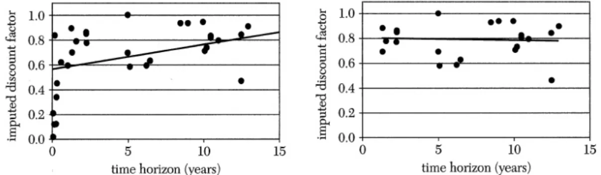
2.1. An illustration of Axiom RD5 (Path Independence). Source: Ok and Masatlioglu (2007, p.221) . . . 7 4.1. Discount Factors and Time Horizons reported by empirical studies. The
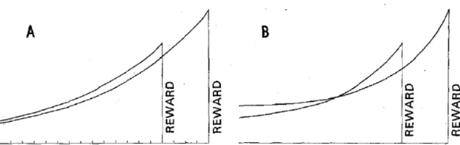
solid line is the least squares t. Source: Frederick, Loewenstein and O'Donoghue (2002, p.362) . . . 31 4.2. "Preference reversals" are ruled out when time is discounted
exponen-tially (subgure A), but occur when time is discounted hyperbolically (subgure B). Source: Ainslie (1975, p.471) . . . 40 4.3. Value functions for three dierent parameter congurations. The value
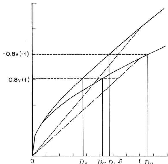
function is steepest around the reference point and greater (in absolute terms) in the area of losses than in the area of gains. Source: al Nowaihi and Dhami (2009, p.227) . . . 45 4.4. Money-Discount Rates for Gains/Losses (equivalent present values) and
Borrowing/Saving (compensating present values). The negative part of the value function was projected into the rst quadrant. Source: Loewenstein and Prelec (1992, p.585) . . . 48 4.5. Eect of omitting "short-run" discount factors on the LS estimation.
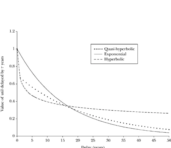
Source Frederick, Loewenstein and O'Donoghue (2002, p.362) . . . 51 4.6. Plot of three absolute discount functions. Source: Angeletos, Laibson,
Repetto et al. (2001, p.51) . . . 52 4.7. Plots of the Relative Discouting Functionη(s, t): Subplots 13 represent
the three transitive time preferences introduced above. The remainder depict intransitive time preferences, two of which are discussed in this thesis. Source Ok and Masatlioglu (2007, p.227) . . . 59 8.1. Illustration of the Three-Period-Consumption/Saving game . . . 81
List of Tables
3.1. Questions in Example 4 of Loewenstein and Prelec (1993) (answers in
parentheses) . . . 21
4.1. Results of the experiment in Thaler (1981) . . . 28
4.2. Questions I and II in Rubinstein (2003) . . . 56
7.1. Writing a term paper: (Discounted) Costs for self 0 and self 1 . . . 71
1. Introduction
Since at least Adam Smith, human's attitude towards time has been of utmost impor-tance to social scientists: Adam Smith himself thought that it determined the Wealth of Nations. Norbert Elias (1988) even went one step further and hypothesizes that a "linear and homogeneous" notion of time is a central pillar of none other than the "civilizing process" of modern man.
Building on Smith's insights, economists John Rae (1834), Eugen von Böhm-Bawerk (1884) and Irving Fisher (1930) sought to analyze the motives that inuenced in-tertemporal decisions. They attributed a central role to impatience - "the marginal preference for present over future goods" (Fisher, 1930, part II, chapter 4). Impatience, in turn was said to be the product of numerous factors objective or subjective in na-ture. Irving Fisher (1930, part II, chapter 4) names the following six subjective factors ("characteristics") that inuence a person's impatience in the obvious directions:
1. Foresight 2. Self-control 3. Habit
4. Expectation of life
5. Concern for the life of other persons 6. Fashion
However, after Paul Samuelson published his "A Note on the Measurement of Utility" in 1937, all these considerations where compressed into the discount factor. Although Samuelson himself raised concern against the overly simplistic formulation of time preferences in this very paper, the vast majority of economic models that involved in-tertemporal decisions adopted his approach, that became known as the "exponentially discounted utility model".
Although the model lacked an empirical or normative foundation, it was not until the 1990s that economists turned to alternative models of time preference in increasing numbers. And quite often, they reverted to the "(neo-)classics" mentioned above.
Part I of the present thesis tries to review some of this recent research in the area of time preferences. The structure is as follows:
1. Introduction
Chapter 2 briey treats the axiomatic derivation of time preferences over outcome-date pairs in general and discusses some of the most important characteristics of time preferences. The following chapter then shows how these can be adopted to model pref-erences over dated streams of outcomes. Chapter 4 presents a number of alternatives to the exponentially discounted utility model and surveys their empirical evidence.
Part II then adopts the least "drastic" among these alternatives (with regard to exponential time preferences) quasi-hyperbolic time preferences and discusses how economic analysis changes: as it turns out, this will have dramatic consequences on the structure of most intertemporal models and will even require a dierent solution concept.
Part I.
Time Preferences
What then is time? If no one asks me, I know what it is. If I wish to explain it to him who asks, I do not know.
2. Classication of Preferences over
Outcome-Date Pairs
In this chapter we give an axiomatic derivation and a characterization of preferences over outcome-date pairs. We will do so along the lines of Ok and Masatlioglu (2007) who came up with a novel approach dubbed 'relative discounting'. Their framework allows for a comprehensive classication of a broad range of time preferences that have been introduced in the literature, while maintaining a certain degree of concrete-ness and cohesiveconcrete-ness. In particular it captures a certain class of non-transitive time preferences.
In section 2.1 we establish the notation and preliminaries, while section 2.2 states and discusses the assumptions necessary for the important theorem of relative discounting. In the last section of this chapter we then examine the implications of characteristics of time preferences, such as transitivity or stationarity. Preferences over streams will be treated separately in chapter 3.
2.1. Preliminaries
In economics, the standard way to analyze time preferences is to model them as binary relations, , over outcome-date pairs. A generic pair being (x, t), where x denotes a 'prize' that is to be obtained in period t. Prizes are undated and are elements of an unidimensional1 outcome spaceX⊆R. In this section it will be convenient to employ
a continuous and innite notion of time, i.e.t∈T = [0,∞). Therefore, preferences are
binary relations over the outcome-date space X ≡X×T.
As usual in this context,(x, t)(y, s) means "not to prefer(y, s)over(x, t)", while
∼denotes that both,(x, t)(y, s) and(y, s)(x, t) hold, which we interpret as "the
decision maker is indierent between (x, t)and (y, s)."
Moreover, let t denote the tth (canonical) projection of , i.e. the ordering of
outcomes that are both due at timet, which we can interpret as the material tastes for outcomes that will be obtained att. Formally,tis dened asxty ⇔ (x, t)(y, t).
In this notation, 0 are for instance the material tastes at time 0.
Following Ok and Masatlioglu (2007, pp.217) we stress that the preferences, denoted by , are the commitment preferences of an agent, i.e. we interpret (x, t) (y, s) as
1Note however, that all results brought forward in this section also generalize to multidimensional
2.1. Preliminaries "if she could commit in period 0 to either 'consume' x in period t or y in period s, she would (weakly) prefer the former". Troughout part I of the thesis we will assume that the decision maker is indeed able to commit to an action in period 0. In part II we will then drop this assumption and discuss the implications. Additionally, we will facilitate the analysis by explicitly ruling out a dimension of risk or uncertainty, i.e. we say that if a the decision maker opts for (x, t) she receives the pair with certainty.
We are now ready to dene time preferences in the following sense (Ok and Masatli-oglu, 2007, p.218):
Denition For an outcome spaceX, a binary relationonX is a time preference
on X, denoted by(X,)if
1. is complete: For every (x, t) and (y, s) inX either (x, t)(y, s) or (y, s)
(x, t) or both (which also implies reexivity).
2. is continuous in the following sense:2 Letan andbnbe convergent sequences
in X in the Eucledian Norm, s.t. am bn, ∀n, then it we require that also limanlimbn has to hold.
3. 0is complete and transitive, where transitivity of0 means that forx, y, z ∈
X: x0y and y0z⇒x0 z. So we assume that the ranking over the goods that are available right now is transitive and complete.
4. 0=t for all t. Therefore the material tastes are the same throughout
time. This restriction explicitly rules out, say, changing tastes as the decision maker becomes older. Likewise, this assumption does not allow for an increased "demand" of for a bottle champagne on New Year's Eve (in the realm of multi-dimensional prizes).
Note that transitivity of does not follow from the transitivity of t. So, the
preferences may generate cycles like (x, t) (x, t+ 2) ∼ (x, t+ 1) ∼ (x, t) but not
cycles like(x, t)(y, t)∼(z, t)∼(x, t). In other words, we restrict ourselves to cycles
that "arise due to the passage of time" (Ok and Masatlioglu, 2007, p. 218). Moreover, the assumptions we make below only permit cycles that involve three or more time periods.
Furthermore, when (X,) is not transitive, we cannot represent the preferences
by a utility function, say, w(x, t), in the usual manner: (x, t) (y, s) ⇔ w(x, t) ≥
w(y, s): for preference relation to be represented by a utility function it necessary
that it is transitive and complete (see e.g. Mas-Colell, Whinston and Green, 1995, 2This concept of continuity is often called "sequential continuity". There is, however, a variety of
other concepts of continuity for binary relations. For an overview see e.g. Baroni and Bridges (2008).
2. Classication of Preferences over Outcome-Date Pairs
p.9). However, as Ok and Masatlioglu showed, we are able to represent them in a dierent way, provided that some additional assumptions hold: Theorem 1 says that
(x, t)≥(y, s)⇔u(x)≥η(s, t)u(y).
2.2. The Relative Discounting Representation and its
Axioms
The following assumptions on(X,)will allow us to represent the time preferences by
a combination of a (static) outcome utility function and a relative discount function, given in 1.
Axiom RD1 (Time Sensitivity): For any x, y∈X and t≥0 there exists ans≥0
s.t. (x, t)(y, s)
Roughly speaking, this assumption ensures that the decision maker will not prefer an outcome-date pair that is delayed by a suciently large amount of time. Implicitly, this assumption already rules out negative time preferences (which would be that the decision maker always favours delays): Suppose for example thatt= 0and thaty0 x,
s.t.(x,0)(y,0). Then, it does not follow from assumption RD1 that delayingymakes it more desireable. Note however, that although this assumption treats delaying and expediting asymmetrically, it does not say that a delay always results in a loss of "attractiveness".
Axiom RD2 (Outcome sensitivity): For any x ∈ X and s, t ≥ 0, there exist
y, z ∈X\{x} s.t. (z, s)(x, t)(y, s)
This assumption is the natural counterpart of axiom RD1 and rules out e.g. lexico-graphic preferences over outcome-date pairs. Intuitively, this axiom states that delay can always be compensated with higher outcomes.
Axiom RD3 (Monotonicity): For anyx, y, z∈Xands, t, r≥0, ift≥randz0 x then(x, t)(y, s)⇒(z, r)(y, s).
This assumption strengthens the antecedents in the way that it brings forward the obvious notion of positive time preferences (or impatience): attributed to human pref-erences since at least Irving Fisher's Theory of Interest (1930): People always prefer sooner pleasures to deferred ones. If we assume for a second thatX is a space of mon-etary outcomes, then assumption RD3 may be bluntly interpreted as: more money is always good whereas delay is always bad.
The next two assumptions guarantee that we can separate the eects of outcomes on preferences from the eects of time in the certain sense of Theorem 1.
Axiom RD4 (Separability): For any x, y, z, w∈X ands1, s2, t1, t2 ≥0 if (x, t1)∼ (y, s1),(z, t1)∼(w, s1)and (x, t2)∼(y, s2)⇒(z, t2)∼(w, s2)
2.2. The Relative Discounting Representation and its Axioms As Ok and Masatlioglu (2007, p.220) put it, axiom RD4 ensures that the premium for delay is separated from the particular reward:
For the sake of argument supposet1 < s1,t2< s2 and that the decision maker told
us that she is indierent between gettingx at periodt1 and gettingyat s1. Therefore
we can think ofy−x >0a premium that is needed to compensate the decision maker
for delaying x fromt1 to s1. Similarly, she can be compensated by a premium w−z
for postponing z from t1 to s1. If we additionally know, that the compensation for
delayingx fromt2 to s2 is also y−x, then axiom RD4 ensures that the compensation
of delaying z is the same as before: w−z.
If we adopt a multidimensional prize space, this assumption ensures that discounting for, say, one's physical health, is the same as discounting for cigarette pus.
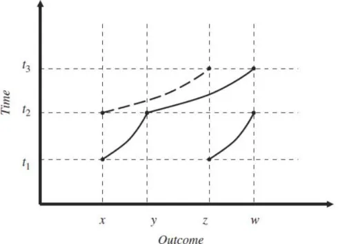
Figure 2.1.: An illustration of Axiom RD5 (Path Independence). Source: Ok and Masatlioglu (2007, p.221)
Axiom RD5 (Path Independence): For any x, y, z, w ∈ X and t1, t2, t3 ≥ 0 if (x, t1)∼(y, t2),(z, t1)∼(w, t2) and (y, t2)∼(w, t3)⇒(x, t2)∼(z, t3)
This path independence property ensures that the aggregate premium for delaying rewards are independent of their order (p.221): For the sake of illustration, suppose that t1 < t2 < t3 and that x < y < z < w (as depicted in gure 2.1). We will now
2. Classication of Preferences over Outcome-Date Pairs
fromt1 tot2 and then again from t2 tot3. In order to make the decision maker willing
to accept these two delays, we have to compensate her with a premium of at leasty−x for the rst delay and then with w−y for the second one. Therefore the aggregate premium involved is w−x.
Second, let consider a dierent order: We start with z and delay it from t1 to t2
requiring a premium of w−z. Next, we postpone x from t2 to t3. The associated
aggregate premium would be (w−z) + (ξ−x).
The aggregate premia are the same if ξ = z, which is precisely what axiom RD5 requires. Since this is quite an unintuitive assumption it is hoped that gure 2.1 brings some clarication.
Axiom RD6 (Monotonicity in prices): 0 is strictly increasing on X.
Axiom RD6 simply states that the elements of X are ordered according to their "attractiveness", which in a sense is a matter of convention.
We are now ready to formulate
Theorem 1 [Relative Discounting] (Ok and Masatlioglu, 2007) Let X be an open interval anda binary relation onX. is a time preference that satises axioms
RD1-RD6, if and only if, there exists an homeomorphism u :X → R++ and a continuous
map η:R2+→R++ such that, for all x, y∈X ands, t≥0,
(x, t)(y, s)⇔u(x)≥η(s, t)u(y), (2.1) where
η(s, t) is strictly decreasing in its rst argument and lim
s→∞η(s, t) = 0 (2.2a)
η(t, s) = 1/η(s, t) (2.2b)
u(x)is increasing. (2.2c)
One important feature of this representation is that given axioms RD1-RD6 hold when evaluating the ranking of two outcome-date pairs, we can separate the "material ranking" from the timing: A static, undated utility u(·) and a relative discount factor
η(·). In the light of this representation, (x, t) (y, s) is then interpreted as (Ok and
Masatlioglu, 2007, pp.222-223):
From the perspective of time 0, the worth at timetof the utility of y that is to be obtained at time sis strictly less than the worth at time t of the utility of xthat is to be obtained at time t.
Again, we stress that these are commitment preferences, i.e. the decision maker commits to her decision in period0.
2.3. Uniqueness Furthermore, we observe that by (2.2b) η(t, t) = 1/η(t, t) ⇒ η(t, t) = 1 since
η(s, t) > 0, which corresponds to the assumption that time does not alter the
ma-terial preferences.
Moreover, our assumption of positive time preferences, i.e. impatience at every period in time, is reected by 0< η(s, t) <1 ⇔ s > t: To see why this holds, suppose rst that 0≤t < s <∞, then by the monotonicity of the discounting term: 0< η(s, t) < η(t, t) = 1Conversely, suppose 0< η(s, t)<1(2.2b)⇒ 0< η(s, t)< η(t, t)(2.2a)⇒ s > t.
Figure 4.7 (on page 59) shows six plots of the relative discount function,η, each one corresponding to a dierent kind of time preference.
2.3. Uniqueness
Theorem 2 [Uniqueness] If a time preference (,X) that satises RD1-RD6 is
represented by (u, η) then it is also represented by (v, θ) if, and only if, v =bua and θ=ηa for a, b >0.
This indicates that the structure of the preferences, imposed by RD1-RD6, restricts the permissible transformations up to simultaneous exponential transformations and multi-plication with a positive constant. In other words, once we xed the functional form of the relative discounting term, the static utility function is unique up to a proportional transformation. Therefore, we have to adopt a concept of "cardinal utiltiy" similar to von Neumann-Morgenstern utility in expected utility theory. But compared with von Neumann-Morgenstern utility we have one degree of freedom less when comparing outcome-date pairs.
2.4. Characteristics of Time Preferences
Theorem 1 is able to deal with a fairly broad class of time preferences. In this section we will discuss how characteristics of time preferences relate to the discount term,η(·,·)
in the relative discount representation.
2.4.1. Transitivity and Absolute Discounting
Up to now, we only assumed the material tastestonX to be transitive. Now we will strengthen this assumption and discuss how "global" transitivity ofonX changes our
analysis. Since "global" transitivity implies transitivity oftfor allt, axioms RD1-RD6
still hold and we are therefore able to analyse such preferences within the framework of relative discounting. On top of that, we expect this assumption to facilitate our analysis and indeed, we observe that the transitivity of time preferences is interrelated with the relative discount function in the following way:
2. Classication of Preferences over Outcome-Date Pairs
η(t, r) =η(t, s)η(s, r) ∀r, s, t≥0 (2.3)
We will show the "if" part of the proof for the case of indierence, "∼":
(x, t)∼(y, s),(y, s)∼(z, r)⇒(x, t)∼(z, r)
which, by Theorem 1⇐⇒
u(x) =u(y)η(s, t), u(y) =u(z)η(r, s)⇒u(x) =u(z)η(r, t)
therefore, η(r, t) =η(s, t)η(r, s)
which, by part (2) of Theorem 1:⇔η(t, r) =η(t, s)η(s, r)
We can therefore exploit the transitivity in order to obtain the usual formulation of absolute discounting, where the time-perspective only enters in an absolute manner (Ok and Masatlioglu, 2007, p.224):
Theorem 3 [Absolute Discounting] Let X be an open interval and a transitive
binary relation on X. Then is a transitive time preference that satises axioms
RD1-RD6 if, and only if, there exist an increasing homemorphism u :X →R++ and
a decreasing and continuous map δ:R+→(0,1] s.t. δ(0) = 1, lim
t→∞δ(t) = 0 and (x, t)(y, s)⇔δ(t)u(x)≥δ(s)u(y) (2.4)
for all outcome-date pairs in X.
Transitivity, as embodied in equation 2.3 allows us to separate the relative discounting function η(s, t) into the quotient of two absolute discount functions: δ(s)/δ(t). Put
dierently, we dene a new function δ(t)≡η(t,0).
From another perspective, the assumption of transitivity together with the deni-tion of time preferences and axioms RD1-RD3 ensure that the condideni-tions of Debreu (1954)'s Theorem II are satised. Therefore, the ranking of outcome-date pairs can be represented by a utility function, say, w(x, t) in the usual manner. The continuity
assumptions of the time preferences even ensure that the utility function is continuous in both arguments. Furthermore, the separability assumptions RD4 and RD5 enable us to write w(·) asδ(t)u(x).3
The notion of absolute discounting (or just "discounting") also gives rise to a dierent interpretation of the preferences: We call the utility associated with an outcome-date pair,δ(t)u(x), the present value ofxand say that(x, t)(y, s)whenever the present
value of x exceeds the present value ofy.
3In the presence of transitivity, one may derive this result with a somewhat simpler set of assumptions.
In particular, one can impose a single separability condition that is less restrictive then RD4 and RD5 (see e.g. the "Thomsen Condition" (condition A6) presented in Fishburn and Rubinstein, 1982).
2.4. Characteristics of Time Preferences Virtually all economic models employ transitive time preferences, the most important being exponential discounting and (quasi-)hyperbolic disounting (see section 4).
2.4.2. The Discount Rate and the Discount Factor
For this class of transitive time preferences it is useful, to describe the shape of the (absolute) discount functions by two measures: the discount rate and the discount factor.
The discount rate describes the "rate of impatience" that is induced by the rate of decline of the discount function. It seems natural to capture this eect by its (negative) instantaneous growth rate, which for discount functions is usually refered to as the discount rate (e.g. Chabris, Laibson and Schuldt, 2008):
Denition In continuous time the discount rate, denoted byρ(t), of a dierentiable
discount function,δ(t), is given by
ρ(t)≡ −δ
0(t)
δ(t) ∀t >0 (2.5)
Obviously, in the case of non-dierentiable discount functions (see e.g. section 4.4) this is not a viable denition. Moreover, if we have a discrete notion of time, we are not interested in the rate of impatience for innitesimal changes in time, but for the change from one period to another4 (Laibson, 2003):
Denition In discrete time the discount rate of a discount functionδ(t)is given by5
ρ(t)≡ −δ(t)−δ(t−1)
δ(t) =
δ(t−1)
δ(t) −1 (2.6)
Another, perhaps more intuitive way to motivate the discount rate is the following: Suppose a decision maker can consumex in period0, giving him a utility of u(x). The
discount rate, ρ(1) tells us, how much more utility (in percentage terms) we have to
oer her, so that she is just indierent between consumingxnow or in the next period. Put dierently, ρ(t) tells about the minimum compensation required for delaying a
4More general, we have to dene the frequency of our observations rst: suppose that time is
mea-sured in years. Then of course, we could decide to partition every year into twelve months. The length of the periods is then given by∆(e.g.∆ = 1/12years). The discount rate is then given
more generally by: ρ(t) ≡ −(δ(t)−δδ((tt−)∆))/∆. As time is measured ner and ner, i.e. ∆ → 0,
the continuous and the discrete formulation coincide. For simplicity, we use the denition where
∆ = 1.
5Note that some authors, e.g. Read (2003), give the alternative denitionρ(t)≡ −δ(t)−δ(t−1)
δ(t−1) , which
2. Classication of Preferences over Outcome-Date Pairs
prize from periodt−1tot. Therefore the discount rate can be interpreted as the "rate of impatience": the higher the discount rate the higher the impatience of the decision maker.
Note, that it follows from assumptions RD1 (time sensitivity) and RD3 (monotonic-ity) that the discount rate ρ(t)is strictly positive in other words the decision maker
always needs a premium so that she is willing to postpone consumption.
By construction, the discount rate is independent of the size of the prize (it only depends on the discount function, which in turn has only time as its argument). This can also be seen as a direct consequence of assumption RD4 (separability), where we explicitly required that the compensation for delay can be seperated from the size of the prize that is to be delayed.
Another useful concept to capture the impatience that is induced by a discount func-tion is the discount factor. Again, we provide the denifunc-tions for both, the continuous and the discrete case:
Denition In continuous time, the discount factor of a dierentiable discount function is dened in the following way (Chabris, Laibson and Schuldt, 2008):
φ(t)≡ lim h→0 1 1 +ρ(t)h h1 = [ lim g→∞ 1 +ρ(t) g g ]−1 =e−ρ(t) ∀t >0 (2.7)
Denition In discrete time, the discount factor is dened in the following way (Laibson, 2003)
φ(t)≡ 1
1 +ρ(t) =
δ(t)
δ(t−1) for t= 1,2, . . . (2.8)
The interpretation of the discount factor in discrete time is straightforward: From the perspective of period0, the discount factor for periodttells us, how much additional discounting is involved between periodt−1 and periodt.
Clearly, assumptions RD1 and RD3 require that0< φ(t)<1, i.e. the decision maker
is always sensitive to additional delay.
Furthermore, note that the value of the discount factor is inversely related to the discount rate: therefore, a high (close to 1) discount factor at periodt+ 1shows that
delaying an outcome for one more period is not perceived as very harmful. On the other hand, a discount factor of close to zero implies that the decision maker does not care much about future satisfaction.
It might seem as a trivial observation, but it will proof to be very useful to note that in discrete time this allows us to write any (absolute) discount function in terms of discount factors: Starting at period0the discounting involved in waiting an additional
2.4. Characteristics of Time Preferences
φ(1) =δ(1)/δ(0) =δ(1) (2.9)
An additional delay of one period gives us δ(1) δ(0) | {z } φ(1) δ(2) δ(1) | {z } φ(2) =δ(2) (2.10)
Iterating brings us to the result that we can write every discount function in terms of discount factors: δ(t) = t Y i=1 φ(i) t= 1,2, . . . (2.11) If it is the case that the sequence {φi}ti=1is decreasing, i.e. φ(t+ 1) < φ(t) then we
can say that from the perspective of period 0the decision maker perceives additional
delays as increasingly harmful and we can therefore say that the rate of impatience is increasing. Conversely, if the sequence is increasing, then the decision maker is more patient for longer planning horizons.
If we plug this representation of the discount function into equation 2.4 of Theorem 3 we yield that fors≥t≥1
(x, t)(y, s)⇔u(x)≥u(y) s
Y
i=t+1
φ(i) (2.12)
Equation 2.12 is of course nothing else but a special case of the relative discount representation given in equation 2.1 for transitive time preferences: here, η(s, t) =
s
Q
i=t+1
φ(i). However, in the case of transitivity, we may interpret η(s, t) as the
condi-tional discount function:
δ(s|s≥t)≡ δ(s)
δ(t) (2.13)
Analogously, also in continuous time we can write (dierentiable) discount functions in terms of discount factors: We take the denition of the discounting rate (equation 2.5) and solve the rst order dierential equation:
−ρ(t)≡ δ
0(t)
δ(t) ∀t >0 (2.14)
2. Classication of Preferences over Outcome-Date Pairs − t Z 0 ρ(τ)dτ+c= ln|δ(t)| (2.15) Cexp − t Z 0 ρ(τ)dτ =δ(t) ∀t >0 (2.16)
normalizing C = 1 gives us the desired result. Again, we observe that an increasing
function of discount factors implies a declining "rate of impatience".
As in the case of discrete time, we can use this identity to express the discount representation of preferences in the following way:
(x, t)(y, s)⇔u(x)≥u(y) exp − s Z t ρ(τ)dτ ∀s > t >0 (2.17)
These observations may seem as tautologies but are clearly a direct consequence of the transitivity of the time preferences: The discounting that is "shared" by two outcome-date pairs, (or: takes place up to periodt) does not play a role in the decision process. We stress that this is not to be confused with stationarity (see following section)!
2.4.3. Stationarity
Stationarity is a feature of time preferences that ensures a certain degree of temporal homogeneity, where the time eect is incorporated only by the dierence between the dates on which prizes are obtained, formally
Denition (Fishburn and Rubinstein, 1982) A time preference on X is called
sta-tionary if
(x, t)(y, s)⇔(x, t+τ)(y, s+τ)
∀(x, t),(y, s)∈ X andτ ∈R s.ts+τ, t+τ ≥0 (2.18)
Within the framework of relative discounting this translates into
Theorem 4 [Stationarity] (,X) is a stationary time preference that satises
2.4. Characteristics of Time Preferences R++ and a decreasing and continuous map ζ:R→R++ s.t.
(x, t)(y, s)⇔u(x)≥ζ(s−t)u(y) ∀(x, t),(y, s)∈ X (2.19)
with lim
a→∞ζ(a) = 0 and ζ(a) = 1/ζ(−a), ∀a≥0
Again, we stress that stationarity should not be confused with the result of equation (2.12): While stationarity means that the only way that timing inuences the ranking of outcome-date pairs is by the dierence of their receival times, transitivity merely requires that it does not matter how much the decision maker only focuses on the eect of the additional delay of the pair that is to be received later. This eect will in general be dierent across time.
Taken together with transitivity this poses enough structure on the time preferences so that the discount functionδ(·)is pinned down to an exponential function. To sketch
why this is the case, note that by stationarity of (,X), (x, t) (y, s) ⇔ (x,0)
(y, s−t). By transitivity and Theorem 3 this holds if, and only ifδ(s)/δ(t) =δ(s−t).
By deningr≡s−tthis can be rewritten toδ(r)δ(t) =δ(r+t), which gives rise to the
conjecture that δ(t) = δt. Since we required 0 < δ(t) ≤1 and that δ is decreasing in
t, it must be the case that 0< δ <1. Moreover, it can be shown that this is the only
continuous and decreasing function that satises the (exponential Cauchy) equation f(s+t) =f(s)f(t).6
The consequences for discounting when both, transitivity and stationarity, jointly hold are summarized in the following Theorem (Ok and Masatlioglu, 2007):
Theorem 5 [Exponential Discounting] Let X be an open interval and be a
bi-nary relation on X. Then is a transitive and stationary time preference that
satises axioms RD1-RD6 if and only if there exists an increasing homeomorphism u:X →R++ and aδ ∈(0,1) s.t.
(x, t)(y, s)⇔δtu(x)≥δsu(y) ∀(x, t),(y, s)∈ X (2.20)
One way to see, that only the dierence of the receival-dates of the outcomes matters, divide both sides of the above equation by δt in order to obtain u(x) ≥ δ(s−t)u(y).
Therefore in the case of transitivity the discounting function ζ(s−t) (see Theorem 4
equals δ(s−t).
One important point is that due to the ambuiguity of the discount representation (see Theorem 2), δ can vary freely in the interval (0,1)unless the discount functionu is xed (up to multiplication with a positive constant).
2. Classication of Preferences over Outcome-Date Pairs
This relatively simple representation of stationary and transitive preferences also gives rise to a dierent interpretation of the discounting term (Manzini and Mariotti, 2007, p. 4): First we rescale the present values by taking logs of the present values which gives
logu(x) +tlogδ ≥logu(y) +slogδ
Dividing by −logδ and dening v(·) ≡ −logu(x) logδ/(whereby we exploit that the utility function is only unique up to multiplication with a positive constant) we obtain the form:
(x, t)(y, s)⇔v(x)−t≥v(y)−s ∀(x, t),(y, s)∈ X (2.21)
2.4.4. Present Bias
One natural counterpart of stationarity is what economists came to call present bias: Special weight is attached to outcomes that are due today. One way7 to formalize this
idea is (Ok and Masatlioglu, 2007, p. 225)
Denition A time preference (,X) exhibits present bias if
(x, t)(y, s) ⇒ (x,0)(y, s−t) ∀x, y∈X, s > t≥0 (2.22)
and if moreover, for anys > t >0there existx, y∈X such that
(x, t)∼(y, s) ⇒ (x,0)(y, s−t) (2.23)
The framework of relative discounting can not only accomodate preferences of that kind, there is also the following connection between a present bias and the relative discounting term:
Theorem 6 [Present Bias] (Ok and Masatlioglu, 2007) (,X) is a time preference
that satises axioms RD1-RD6 and has present bias if, and only if, is represented
by some (u, η) s.t. η(s, t) ≥ η(s−t,0) holds whenever s > t > 0 for all with strict
inequality (>) for some dates.
When a time preference exhibits present bias, we can therefore say that the dierence in the timing of two future outcomes is certainly not getting less important when both are speeded up so that the sooner one is can be obtained today. In the class of transitive time preferences that allow for an (absolute) discount representation, this translates to a lower discount factor at period 0 than at other points in time:
2.4. Characteristics of Time Preferences Present biased time preferences are one form of time preferences that allow for "pref-erence reversals". For some outcome-date pairs (x, t) and (y, s) the preferences are
reversed when both outcomes are delayed or speeded up. The classic example is due to Thaler (1981): Although a decison maker might choose one apple today over two apples tomorow, she as well might choose two apples in 101 days over one apple in 100 days. Stationarity on the other hand would require that she picked one apple in both choices: Applying the denion of stationarity as given in equation 2.18 yields
(one apple,0 days)(two apples,1 day)⇒
(one apple,0 + 100 days)(two apples apple,1 + 100 days) (2.24)
The simplest type time preferences that exhibit such a present bias is called "quasi-hyperbolic" time preference and is discussed in section 4.4.
3. Time Preferences over Innite
Streams of Outcomes
So far we discussed preferences over outcome-date pairs. In this chapter we will focus on preferences over dated streams of outcomes, which we will sometimes call "schedules". Also in this chapter, we will restrict ourselves to deterministic streams and assume that the decision maker has commitment power, i.e. once the decision maker has made a decision, she cannot alter it as time goes by. Therefore it suces to analyze the decision makers preferences at time 0. From now on we will restrict ourselves to the
case of discrete time, whenever possible.
We say that a stream of outcomes attributes an outcome at ∈At⊆Rn to every point in time t ∈ T. We employ a discrete notion of time i.e. break down time into periods of equal length: T = N0. Furthermore, we require the outcome space to be
the same in every periodAs=At=A ∀s, t∈T. A stream of outcomes, or schedule,
a= (a0, a1, . . .), is an element ofQt≥0A≡ A, where
Qdenotes the cartesian product.
Sometimes we will denote parts of streams that start in period s(and end in periodt) withsa(sat).
In economics, streams are for example, bundles of goods (at)t≥0 where at = (at1, at2, . . . , atn)∈ Rn+. In a broad range of dynamic models economists conveniently
assume that there is only a single consumption good ct ∈ R+. Due to the innite
number of periods, the decision maker is often called "dynasty".
3.1. Aggregation of Present Values
Ever since its introduction by Paul Samuelson in 1937, the overwhelming majority of economics models implemented preferences over such innite streams in the following way, which is often referred to as "additive discounted utility" or simply "discounted utility" (DU) representation of the preferences over streams:1
ab⇔X t≥0 δ(t)u(at)≥ X t≥0 δ(t)u(bt) ∀a, b∈ A (3.1)
with0< δ(t)<1 fort >0 andδ(0) = 1.
1see Weibull (1985) for the derivation of a "general discount representation" of preferences over
3.1. Aggregation of Present Values
3.1.1. Intertemporal Noncomplementarity
As we will see, this is of course the most straightforward way to model time preferences over innite streams of outcomes. But despite its popularity it was not until the 1960's that economists started to provide an axiomatic foundation, which indicated a highly restricted domain:
With respect to the classication in section 2.4 one assumes transitivity over date-outcomes pairs, so that their rankings can be represented by their present value, δ(t)u(at), whereδ(t) is for example one of the discounting functions, discussed in
sec-tion 4 Samuelson himself formulated the DU model with an exponential discounting function. In addition we postulate (Weibull, 1985):
Axiom S1 (strict intertemporal noncomplementarity): For every a, b, c∈ A it
holds that
ab⇔a+cb+c (3.2)
Note that up to now, intertemporal complementarities were not an issue, since the decision maker received only single outcomes that were mutually exclusive: She either gets (x, t) or (y, s). In the realm of streams, however, there is room for this highly
disputed assumption: As Koopmans (1960), who was probably the rst to come for-ward with an axiom like this, put it, "[o]ne cannot claim a high degree of realism for such a postulate, because there is no clear reason why complementarity of goods could not extend over more than one time period." Samuelson (1952, p.674) made this point somewhat more crisply: "The amount of wine I drank yesterday and will drink tomor-row can be expected to have eects upon my today's indierence slope between wine and milk."
3.1.2. Critique: Habit Formation and Anticipated Utility
Concerns like these motivated economists (e.g. Constantinides, 1990) to study con-sumption under habit formation: Roughly speaking, habit formation tries to capture the eect that over time, people get used to a certain standard of consumption, a habit, therefore consumption in one period also directly inuences the marginal utility of future consumption. Wathieu (1997) used a model model of habit formation in a nite time-framework to explain some of the anomalies of the exponential discounting model discussed in section 4.1.
Other authors adopted a similar approach but posited models where individuals also gain gratication from the anticipated utility (Frederick, Loewenstein and O'Donoghue, 2002, p.371). To indicate how this can be formulated formally, let c ∈ A denote,
say, an innite consumption stream and v(ct) be the utility derived from "actual"
3. Time Preferences over Innite Streams of Outcomes
t is given byu(tc) =v(ct) +α(γv(ct+1) +γ2v(ct+2). . .with γ <1. This introduction
of anticipated utility of course implies that people will sometime voluntarily in fact postpone gratications into the future.
This is also consistent with the ndings of Loewenstein and Sicherman (1991), who confronted subjects with several wage proles, some of them decreasing, some of them increasing. The overwhelming majority of the respondents chose an increasing wage prole, even after being made aware of the fact that via appropriate saving the decreas-ing wage proles could be converted into wage proles that dominated the increasdecreas-ing ones. Unusual in the profession of economics, Loewenstein and Sicherman chose to report the respondent's reasons for choosing the increasing wage proles. A large frac-tion reported either an "aversion of decrease", "inafrac-tion" or an (intrinsic?) "pleasure from increase".
3.1.3. Critique: Preference for Spreading Consumption
Loewenstein and Prelec (1993) argue that psychologically, individuals perceive choices over sequences of outcomes fundamentally dierent from choices over outcome-date pairs. They argue that decision makers have an intrinsic preference for the spread of consumption within a given period. They support this hypothesis by a series of mini-studies, two of which we will discuss here:
In one mini-study (Prelec and Loewenstein, 1991, p.95-96) they asked respondents the following question (original phrasing given):
Suppose you were given two coupons for fancy dinners for two at the restau-rant of your choice. The coupons are worth up to $100 each. When would you choose to use them? Please ignore considerations such as holidays, birthdays, etc.
The authors told one group that the coupons were valid for two years and another group that the coupons were valid for four years. Yet another group was given no constraint. On average, subjects that were given a constraint scheduled both dinners later than the control group (the one without an explicit constraint), conrming the hypothesis.
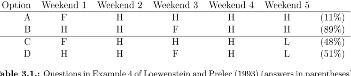
In another mini-study (Loewenstein and Prelec, 1993, example 5) presented subjects with the following pairs of questions (original phrasing given):
Imagine that over the next ve weekends you must decide how to spend your Saturday nights. From each pair of sequences of dinners below circle the one you would prefer. "Fancy French" [F] refers to dinner at a fancy French restaurant. "Fancy lobster" [L] refers to an exquisite lobster dinner at a four-star restaurant. Ignore scheduling considerations (e.g., your current plans).
3.2. Intergenerational Equity and Impatience The authors assumed that the subjects ate at home [H] on the remaining weekends. The results of this study are presented in table 3.1.
Option Weekend 1 Weekend 2 Weekend 3 Weekend 4 Weekend 5
A F H H H H (11%)
B H H F H H (89%)
C F H H H L (48%)
D H H F H L (51%)
Table 3.1.: Questions in Example 4 of Loewenstein and Prelec (1993) (answers in parentheses)
When asked to choose between options A and B the majority chose B, a result which the EDU model rationalizes with a negative rate of impatience, but can also be made sense of by insinuating a preference for spread. This hypothesis is conrmed when in addition to the fancy-french dinner, a lobster-dinner is scheduled on weekend 5: Suddenly the option where the french dinner is scheduled earlier becomes more attractive. The authors obviously interpreted the result in the way that adding the lobster dinner triggered a preference for spread of consumption and made some people chose the option with the french dinner on weekend 1.
The authors interpret both results as a straightforward violation of axiom S1 (strict intertemporal noncomplementarity) and suggest that the preferences over streams are in fact qualitatively dierent from preferences over outcome-date pairs in the sense that decision makers exhibit an intrinsic preference for spreading consumption.
Although these studies could easily be dismissed as circumstantial evidence and explained by entirely dierent factors (for instance the imputed income eect from adding a lobster dinner), the hypothesis is conrmed by our intuition.
3.2. Intergenerational Equity and Impatience
Axiom S1 makes it possible to aggregate the (static) utilities of every point in time and we can simply sum up over all present values the outcomes. For this reason, it is also admissible to speak of innite utility streams (Diamond, 1965, see e.g.). This in itself brings about another issue: Since we sum over an innite number of periods, it does not follow from any of the assumptions we made so far that
− ∞<X
t≥0
δ(t)u(at)<+∞ (3.3)
So, if the limit does not exist, we cannot infer the ranking of two streams from simply comparing their accumulated present values. This motivated economists to employ a so called overtaking criterion to evaluate streams with innite utility (Acemoglu, 2009,
3. Time Preferences over Innite Streams of Outcomes
p.261): From a set of alternative streams, the decision maker is said to choose the stream that gives a higher payo at all times from a certain (nite) period onwards.
This problem of "innite utility" also has implications of a dierent kind: Suppose that the static utility of each period corresponds to the well-being of a generation. We then aggregate them into a function, which we interpret as a "social welfare function", W, of, say, a country, that maps innite utility streams into the real numbers. We require social welfare functions to satisfy the following (innocuous) axioms:
• (Weak) Pareto: Whenever it holds for two utility streams, that all generations
are strictly better o, i.e. obtain higher utility from one stream, a, than in the other b, it follows that W(a)> W(b).
• Intergenerational equity: W does not discriminate between the generations in the sense that if two generations "swap" their levels of utility, it leaves the social welfare function unchanged.2
• Continuity in the sup-metric3
From Koopmans (1960) and Diamond (1965) onwards a number of studies showed that there is no social welfare function that jointly satises all three axioms: "Intu-itively, the reason is that if there is in all circumstances a preference for postponing satisfaction-or even neutrality toward timing- then there is not enough room in the set of real numbers to accommodate and label numerically all the dierent satisfaction lev-els [...][of] an innite future." (Koopmans, 1960, p. 288). In a more recent paper Basu and Mitra (2003) showed that the Pareto Axiom alone precludes an equal treatment of all generations.
3.3. An Alternative Approach
In section 3.1 we derived time preferences over innite streams that were induced by time preferences over outcome-date pairs. We will now approch the issue of intertem-poral utility of innite streams from a dierent, perhaps more natural vantage point: We do not explicitly assume that axioms RD1-RD6 hold, so in a sense we will start from scratch and follow Koopmans (1960) in his axiomatic derivation of preferences over innite utility streams. Our goal is to derive preferences over innite streams directly (i.e. not as induced by preferences over outcome-date pairs). In addition to axiom S1 Koopmans makes the following assumptions:
2This particular notion of intergenerational equity is often refered to as the "anonymity axiom" (see
e.g. Basu and Mitra, 2003, p.1559).
3Due to the innite number of periods, streams are elements of an innite dimensional vector space,
3.4. Uniqueness K1 (Continuity): The preference relation(,A)can be represented by a continuous
(in the sup-metric) utility function
This implies transitivity, completeness and continuity ofinX.
K2 (Sensitivity): The utility function is sensitive to changes in any period-utility. In the case of period 0 this requires that there existc0 andc00∈As.t.(c0, 1a)(c00, 1a)
for all 1a. This assumption not only excludes the trivial case where the decision maker
is indierent between all streams, but also excludes the (somewhat pathological) case of a decision maker, who has the following "heroic" (Koopmans, 1960, p.291) preferences:
U(a) = lim
τ→∞ ( supt≥τ(at)) (3.4)
Further, we assume a form of temporal homogeneity in the form of
K3 (Stationarity of innite streams): for all c0 and alla, b∈ Ait holds that: (c0, a)(c0, b)⇔ab (3.5)
As in section 2.4.3 stationarity of streams says that the ranking of the alternatives does not change as both of them are speeded up or delayed by the same number of periods.
This allows us to write the utility functionU in the form
U(0a) =V(u(a0), U(1a)) (3.6)
where V(·) is called the aggregator function that can be shown to be continuous
and increasing in both of its arguments: u (instantaneous utility) and U (prospective utility). The crucial point is, that due to stationarity, neitheru, nor U are dependent on time! This recursive form gives rise to the idea of dynamic programming, which we will make use of heavily in part II of this thesis.
Moreover, it follows that the decision maker has to exhibit a sucient degree of impatience, in the sense that less weight is given to future utility as to immediate utility. Otherwise the previous axioms are incompatible with each other.
3.4. Uniqueness
In the case of streams the static utility function u(·) is comparable to von
Neumann-Morgenstern utility functions in the sense that it is unique up to positive linear trans-formations. Formally, we say that the preferences over streams of outcomes, denoted by (,A), that can be represented by the additive discount representation(δ, u):
3. Time Preferences over Innite Streams of Outcomes ab⇔X t≥0 δ(t)u(at)≥ X t≥0 δ(t)u(bt) ∀a, b∈ A (3.7)
can also be represented by an additive discount representation(δ, v)wherev=ku+d and k >0. The main reason for this result is the linearity of the summation operator.
4. Types of Time Preferences and their
Empirical Evidence
In this chapter we discuss a number of time preferences that have been introduced in the literature. The rst section will be devoted to the "top-dog": the exponentially discounted utility (EDU) model. Ever since its introduction by none other than the late Paul Samuelson it has been the most widely used model of intertemporal choice. But from the 1960s onwards, empirical evidence was mounting up against this model and the list of "anomalies" that the EDU model failed to explain became longer and longer. In section two we will review these ndings and discuss in greater detail the issue of measuring discount rates empirically. The evidence led to a spate of papers that proposed to adopt dierent (absolute) discount functions that are hyperbolic in shape and that could explain most of these "anomalies". Two of these alternative discount functions will be discussed in sections three and four. As we will see, the empirical evidence does not point unequivocally in their direction if assessed critically. The following two sections will then provide us with models of time preferences that dier from the EDU model even more in the sense that they drop the assumption of transitivity, but still have a relative discount representation, i.e. they can be incorpo-rated into the framework introduced in chapter 2. This will not be possible anymore in the case of the two types of time preferences discussed in sections seven and eight, which is why they therefore serve as examples of time preferences that violate one or more of the axioms of relative discounting.
4.1. Exponential Discounting
The exponential discount function is given by
δE(t)≡δt δ ∈(0,1) (4.1)
As we saw in chapter 2 the exponential discount function (EDF) is the only discount function that represents time preferences that are both, stationary and transitive. Due to the stationarity it exhibits a constant discount rate. Therefore, it is in a sense formulated in an analogy to a constant interest rate: In every period, the decision maker can be compensated for an additional delay of a prize x that gives static utility of u(x) by an increase of ρu(x). Therefore the decision maker exhibits the same rate
4. Types of Time Preferences and their Empirical Evidence
of impatience, independent of the planning horizon. Conversely, the discounted value or present value of a prize x that is obtained in periodtis simply given by
1 1 +ρ
t
u(x) (4.2)
The second measure of impatience introduced in section 2.4.2 was the discount factor, φ(t). The discount factor of the exponential discount function is given by
φE(t)≡ δE(t) δE(t−1) = δ t δt−1 =δ ∀t >0 (4.3)
that is, the discount factor is also constant across time. Moerover, it is relatively easy to show that the exponential discount function is the only discount function that exhibits a constant discount factor φ:
Proof
φ(t)≡ δ(t)
δ(t−1)=φ
δ(t) =φδ(t−1) (4.4)
Soδ(t) has to be a solution to the homogenous rst-order linear dierence equation
with constant coecients. The general solution of this dierence equation is given by:
δ(t) =bφt (4.5)
The intial value problem is δ(0) = 1 and xes b = 1, which gives us the solution
δ(t) =φt. Moreover, sinceδ(t) is a discount function, we require δ(t)to be decreasing
and nonnegative. These two conditions together imply that φ ≡ δ ∈ (0,1), which
brings us to the exponential discount function and completes the proof.
Since the EDF represents transitive time preferences over outcome-date pairs, it may also be used to represent preferences over innite streams. Plugging the exponential discount function into equation (3.1) gives us the exponentially discounted utility model (EDU): ab⇔X t≥0 δtu(at)≥ X t≥0 δtu(bt) ∀a, b∈ A (4.6)
On as few as seven pages this model was introduced by Samuelson and given an axiomatic foundation by Koopmans (1960) (see section 3.3). Owing its popularity perhaps to its simplicity, the exponentially discounted utility model was adopted in virtually every model that involved intertemporal trade-os: from project evaluation to
4.2. On Eliciting Time Preferences micro-funded growth models. The manifold applications nonwithstanding, Samuelson himself saw the model merely as a starting point for further research and certainly did not endorse its widespread use as the following quote shows:
In conclusion, any connection between utility as discussed here and any welfare concept is disavowed. The idea that the results of such a statistical investigation could have any inuence upon ethical judgments of policy is one which deserves the impatience of modern economists. (Samuelson, 1937, p.161)
Moreover, neither Samuelson nor any other author ever adopted the exponential dis-counting function on empirical grounds or even pretended that it is a realistic model. On the contrary: in their axiomatic derivation of the exponential discounting repre-sentation Fishburn and Rubinstein say that "[they] know of no persuasive argument for stationarity as a psychologically viable assumption." (p.681).
In the next session we will assess how the exponentially discounted utility model holds up against reality.
4.2. On Eliciting Time Preferences
From about 1980 onwards economists and psychologists sought to infer discount rates from human1 decisions. From hindsight, the rst tentative steps to do so were not
particularly successful in identifying the discount rates. But before we discuss in detail the issue of eliciting discount functions (see section 4.2.2) it may be useful to have a look at one of the pioneering studies, in particular since they are still quoted as a motivation for adopting discount functions that dier from the exponential one. We are therefore going to discuss the ndings of Thaler (1981):
4.2.1. The rst tentative steps
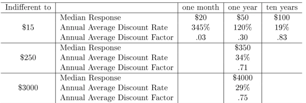
Thaler asked respondents the hypothetical question of how much money they had to be given in one month/one year/ten years in order to be indierent to receiving $15 now. In addition, he asked subjects, about the dollar amount that would make them indierent to getting $250 and to getting $3000 in a year. The median responses and the implied discount rates are given in table 4.1.
Thaler calculated separately the average annual discount rates for each response given. He did so in the following way (Frederick, Loewenstein and O'Donoghue, 2002): In the case of ($15, now) ∼ ($50, one year) this means that$15 = δ(one year)$50.
Using the identity that we can express every discount function as a product of its dis-count factors (equation 2.17) the average annual disdis-count rate is then given by the
4. Types of Time Preferences and their Empirical Evidence
Indierent to one month one year ten years
$15 Median ResponseAnnual Average Discount Rate 345%$20 120%$50 $10019% Annual Average Discount Factor .03 .30 .83 $250 Median ResponseAnnual Average Discount Rate $35034%
Annual Average Discount Factor .71 $3000 Median ResponseAnnual Average Discount Rate $400029%
Annual Average Discount Factor .75
Table 4.1.: Results of the experiment in Thaler (1981)
equation: $15 = exp(−ρ1)$50Soρ= 1.20. Analogously,$15 = exp(−3.45 1/12)$20 = exp(−.19 10)$100. That is we calculate an average discount rate as if the discount
rate were constant in the interval for given time horizons: Therefore, Rt
0
ρ(τ)dτ =ρt. Alternatively we could calculate average per period discount rates: If we already now, that the average discount rate for a one month horizon is 345%, then the average discount rate in the period of between one month from now to one year from now is given by the equation $15 = exp(−3.45 1/12) exp(−ρ 11/12)$50. So ρ equals 100%. Likewise, a similar calculation yields that the average discount rate for the period starting at one year from now and ending ten years from now is about 7.7%.
These results suggest that discount rates decline in both, the planning horizon and the money involved.
4.2.2. Methodology
After having discussed the particular approach of Thaler (1981), it may be a good idea to lay out in a more general fashion, how one can measure time preferences. There is of course a large number of possibilities to elicit (average) discount rates from decisions: First of all, these decisions can be either observed in real life or in a laboratory environment.
Studies that base their estimations of discount rates on data from real life experience are often called eld studies. One of the rst studies to infer discount rates from real world decisions that involved intertemporal trade os, was conducted by Hausman (1979) who collected data about the purchase of air conditioners: The intertempo-ral trade-o was given by the fact that the lower priced air conditioners had larger operating costs.
By the same token, the termination of about 66 000 military servicemen provided a cause for rejoicing for economists Warner and Pleeter: The employees faced the choice
4.2. On Eliciting Time Preferences of either accepting a lump-sum payment of about $25 000 or an annuity that - on the basis of a seven-percent interest rate - was "worth" about $50 000. The overwhelming majority chose the lump-sum payment, which can only be rationalized within the EDU-model if the average discount rates were at least 17%. In nominal terms, this saved the government about $1.7 billion in compensations.
One important drawback of eld studies is that it may be dicult to isolate the eect of time preferences from other considerations: In the case of Hausman's study one could for instance argue that decision makers were not aware of the operating costs in the rst place or that individuals simply found themselves liquidity constraint.
Therefore, the majority of studies tried to elicit discount rates in in experimental situations in order to control the decision environment and suppress the "background noise" of other economic considerations. These lab-experiments range from hypo-thetical "paper-and pencil" tests to experiments involving sizable monetary rewards. Frederick, Loewenstein and O'Donoghue (2002, p.386-389) distinguish between four dierent experimental procedures:
• Choice Tasks: In the case of choice tasks subjects are given the choice between
two outcome-date pairs, where one outcome is smaller and due sooner than an-other one that is larger but due later. Suppose for instance that the smaller amount is $100 due today, whereas the other amount is $120 due in one year. If the subject choses the smaller, sooner amount, then the experimenter concludes that the discount rate is at least 20%. In order to narrow down the discount rate to a single number, subjects are often given a series of choices.2 That in
itself brings about the problem of the so called anchoring eect: suppose for instance that there are two test schedules, each consisting of two questions. One test schedule rst gives the subject the choice between $100 now vs. $103 next year and then the choice between $100 now vs. $120 in one year. In the other schedule, the second question is the same, but the rst question gives the choice between $100 now vs. $140 next year. The anchoring eect states that subjects tend to stick to the decision, "the anchor", they made in the rst round and therefore a person is more likely to choose $100 over $120 in the rst schedule than in the second.
• Matching tasks ask people for the corresponding value $x that would make
them indierent between, say, $100 now and $x in one year. The study of Richard Thaler (1981) discussed above elicited discount rates in this manner. The advantage over choice tasks is that it gives one discount rate and excludes 2In a recent paper, Chabris, Laibson, Morris et al. (2008) also recorded the response time of subjects,
i.e. the time it took subjects to answer questions. The authors surmise that longer response times indicate that subjects found it harder to give a ranking of the two options and therefore the two are perhaps perceived to be more similar.
4. Types of Time Preferences and their Empirical Evidence
the anchoring eect. The disadvantages are that subjects tend to give very crude responses that are just mulitples of the other outcome (here: n∗$100)
• In rating tasks subjects have to indicate the attractiveness of an outcome
date-pair. In the case of a transitive model of time preferences this can be thought of as a proxy for the utility (the present value) of an outcome-date pair (i.e. δ(t)u(x)).
• Pricing tasks are similar to rating tasks but ask subjects for their willingness
to pay for a dated outcome.
Although it is not clear of wether it makes much of a dierence (see e.g. Frederick, Loewenstein and O'Donoghue (2002) on this issue) to use either real or hypothetical rewards in experiments, it is certainly the case that studies that involve real rewards have to be incentive compatible: Just image matching tasks were people demand ridicu-lously huge sums in order to be compensated for a single day of delay. From a dierent perspective, the experimental procedures should be seen as mechanisms that should implement truthtelling. Therefore it seems only natural to resort to the best known mechanisms in economics: auctions. Manzini and Mariotti (2007) list three dierent types of auctions where truthtelling is a (weakly) dominant strategy:
• Second Price Sealed Bid (Vickrey) auction: The bidder that places the
highest bid wins the prize, but pays the only the bid of the second highest bidder. It can be easily shown that truthtelling (here: stating the "correct" discount rate or indierence outcome) is a weakly dominant strategy. In addition, this auction format has the advantage that it is relatively easy to understand and "close" to a direct mechanism (i.e. an incentive compatible mechanism where the strategy space of the agents is identical to the type space)
• English (ascending bid) auction: The price of the good to be auctioned o
increases steadily with time. Bidders may drop out at any time. When only one bidder is left, the auction stops and the remaining bidder gets the item at the last price. This auction is strategically equivalent to the Second Price Sealed Bid auction.
• Becker-DeGroot-Marschak (BDM) procedure: The decision maker "plays
against" a uniform probability distribution. When the price drawn is lower than the price stated by the decision maker, she obtains the item for the price drawn, otherwise she gets nothing.
Note that while the rst two auctions are robust to risk-aversion, the third one is not. Although experimenters usually put a lot of emphasis on explaining the procedures to the subjects, one might doubt wether this really implements the desired outcomes.
4.2. On Eliciting Time Preferences Furthermore, Manzini and Mariotti (2007, p.20-21) argue that "these elicitation meth-ods suer from serious incentive [problems] in the neighborhood of the truth telling [...] strategy: deviations may be 'cheap' enough".
4.2.3. Findings - Four "Anomalies" of the EDU model
A myriad of studies (Hausman, 1979; Benzion, Rapoport and Yagil, 1989; Kirby, 1997, just to mention a few) elicited discount rates in one of the ways described above. These studies were thought to document patterns that constitute "anomalies" of the (E)DU model. The most cited of these anomalies are the following (Loewenstein and Prelec, 1992):
Decreasing Discount Rates
Subsequent studies conrmed the ndings of Thaler (1981): The average discount rates are strictly declining with time horizon. This implies that the discount rates themselves, ρ(t) are also declining with time. Conversely, the discount factor, φ(t) is
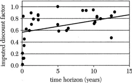
increasing with time. In other words, individuals are more patient for longer planning horizons. In their meta-study, Frederick, Loewenstein and O'Donoghue (2002) evaluate the reported discount rates of a plethora of studies. They then regressed the discount rates against the reported time horizon and found that across studies the discount factors increase with the time horizon (see gure 4.1).
Figure 4.1.: Discount Factors and Time Horizons reported by empirical studies. The solid line is the least squares t. Source: Frederick, Loewenstein and O'Donoghue (2002, p.362)
4. Types of Time Preferences and their Empirical Evidence The (absolute) Magnitude Eect
The Magnitude Eect says that discount rates are lower for higher amounts of money relative the small amounts of money. As mentioned above, the magnitude eect can also be observed in the data presented by Thaler: The average one-year discount rates decline with the dollar amounts: Whereas the median annual discount rate for the $15 prize was a whopping 120%, increasing the stakes to $250 and $3000 yielded by far lower discount rates of 34% and 29%, respectively. More elaborate studies (e.g. Benzion, Rapoport and Yagil, 1989) reproduced these results.
The Sign Eect
The Sign Eect or Gain-Loss Asymmetry captures the pattern found in experimental evidence that decision makers discount losses at a lower rate than gains. Sometimes this eect is so pronounced that researches reported negative discount rates for losses. Loewenstein and Prelec (1992, p.575) present evidence from earlier studies were re-spondents, on average, were indierent between receiving $10 now and reiceiving $21 in one year, implying an average annual discount rate of 110%. In the case of losses on the other hand, individuals declared to be indierent between losing $10 now and losing $15 one year later on average, implying a discount rate of only 50%.
The Delay-Speedup Asymmetry
Several studies (for instance Loewenstein, 1988) documented a framing eect that is present in intertemporal choice: In a typical study respondents are asked two questions: in question number one, they are asked for the minimum amount required to be willing to delay the receipt of, say, $100 from period s to period t. Suppose that this premium is $x. In question number two they are asked to speed up the receipt of $100+x from period t to period s. As it turns out, the amount required for delay is by far larger (about three to four times) than the amount required for speeding up consumption. The choice pairs, however, are clearly the same: (100, s) and(100 +x, t), respectively.
4.2.4. Critique: Confounding Factors
Although most of these anomalies are robust ndings across studies, it may be a good idea to pause for a second and assess what these studies are actually measuring. In recent years various scholars raised their concerns wether the empirical ndigs really manage to identify time preferences, or if the ndings are merely due to other, con-founding factors. Frederick, Loewenstein and O'Donoghue (2002) mention the following points of critique:
4.2. On Eliciting Time Preferences Risk Aversion/Concave Utility Functions
The most important challenge to the ndings is that almost all of the empirical studies explicitly or implicitly assumed risk neutrality of the agents. Within the context of the normative von Neumann-Morgenstern theory of decision under risk, an agent is risk neutral if and only if her preferences over certain monetary outcomes can be represented by a linear utility function. As mentioned in chapter 3, von Neumann-Morgenstern utility functions are only unique up to monotone ane transformations. Therefore, the utility function over static and certain monetary outcomes can be written as the identity function,u(x) =x, without loss of generality. In words, the decision maker values every additional euro the same. As a consequence, the wealth level of an economic agent can be ignored in the analysis of decision under risk: it does not matter if the rst or the 1000th $ is at stake. By the same token, the baseline consumption is also not important when evaluating the ranking of two outcome-date pairs, each one of which increasing consumption on top of the baseline consumption level. We will now discuss the possible implications on the measurement of discount rates, when the assumption of risk neutrality is violated.
Most studies try to measure the present value of outcome-date pairs in one of the following two ways (Loewenstein and Prelec, 1992, p.576).
They either try to elicit the equivalent present value of a delayed outcome, (x, t),
which we denote by ψ(x, t). It is usually dened implicitly as:
u(c+ψ) +δ(t)u(c) =u(c) +δ(t)u(c+x) (4.7)
In words, the equivalent present value is the increase in immediate consumption that makes the decision maker indierent to x additional units of consumption later. Ex-plicitly, ψ(x, t) is then given by
ψ(x, t)≡u−1[(1−δ(t))u(c) +δ(t)u(c+x)]−c (4.8) Alternatively, experimenters elicited the compensating present value, κ(x, t), which
is (implicitly) dened as:
u(c−κ) +δ(t)u(c+x) =u(c) +δ(t)u(c) (4.9)
Let us focus on the equivalent present value, ψ(x, t): As we saw in the case of
Thaler (1981) experimenters then obtained their estimates of discounting by dividing the equivalent present value by x. Noor (2009a, p.871) refers to this function as the money-discount function:
D(x, t)≡ ψ(x, t)
4. Types of Time Preferences and their Empi