A Review on Multi-Label Learning Algorithms
Min-Ling Zhang and Zhi-Hua Zhou,
Fellow, IEEE
Abstract
Multi-label learning studies the problem where each example is represented by asingle instance while associated with a set of labels simultaneously. During the past decade, significant amount of progresses have been made towards this emerging machine learning paradigm. This paper aims to provide a timely review on this area with emphasis on state-of-the-art multi-label learning algorithms. Firstly, fundamentals on multi-label learning including formal definition and evaluation metrics are given. Secondly and primarily, eight representative multi-label learning algorithms are scrutinized under common notations with relevant analyses and discussions. Thirdly, several related learning settings are briefly summarized. As a conclusion, online resources and open research problems on multi-label learning are outlined for reference purposes.
Index Terms
Multi-label learning, label correlations, problem transformation, algorithm adaptation.
I. INTRODUCTION
Traditional supervised learning is one of the mostly-studied machine learning paradigms,
where each real-world object (example) is represented by a single instance (feature vector)
and associated with a single label. Formally, let X denote the instance space and Y denote the label space, the task of traditional supervised learning is to learn a function f : X → Y
from the training set {(xi, yi) | 1 ≤ i ≤ m}. Here, xi ∈ X is an instance characterizing the properties (features) of an object and yi ∈ Y is the corresponding label characterizing its
Min-Ling Zhang is with the School of Computer Science and Engineering, and the MOE Key Laboratory of Computer Network and Information Integration, Southeast University, Nanjing 210096, China. Email: [email protected].
Zhi-Hua Zhou is with the National Key Laboratory for Novel Software Technology, Nanjing University, Nanjing 210023, China. Email: [email protected]. (Corresponding author)
semantics. Therefore, one fundamental assumption adopted by traditional supervised learning is
that each example belongs to only one concept, i.e. having unique semantic meaning.
Although traditional supervised learning is prevailing and successful, there are many learning
tasks where the above simplifying assumption does not fit well, as real-world objects might be
complicated and have multiple semantic meanings simultaneously. To name a few, in text
cate-gorization, a news document could cover several topics such as sports, London Olympics, ticket
salesand torch relay; In music information retrieval, a piece of symphony could convey various
messages such as piano, classical music, Mozart and Austria; In automatic video annotation,
one video clip could be related to some scenarios, such as urban and building, and so on.
To account for the multiple semantic meanings that one real-world object might have, one
direct solution is to assigna set of proper labels to the object to explicitly express its semantics.
Following the above consideration, the paradigm of multi-label learning naturally emerges [95].
In contrast to traditional supervised learning, in multi-label learning each object is also
repre-sented by a single instance while associated with a set of labels instead of a single label. The
task is to learn a function which can predict the proper label sets for unseen instances.1
Early researches on multi-label learning mainly focus on the problem of multi-label text
categorization [63], [75], [97]. During the past decade, multi-label learning has gradually attracted
significant attentions from machine learning and related communities and has been widely applied
to diverse problems from automatic annotation for multimedia contents including image [5], [67],
[74], [85], [102] to bioinformatics [16], [27], [107], web mining [51], [82], rule mining [84],
[99], information retrieval [35], [114], tag recommendation [50], [77], etc. Specifically, in recent
six years (2007-2012), there are more than 60 papers with keyword multi-label (or multilabel)
in the title appearing in major machine learning-related conferences (including ICML/ECML
PKDD/IJCAI/AAAI/KDD/ICDM/NIPS).
1
In a broad sense, multi-label learning can be regarded as one possible instantiation of multi-target learning [95], where each object is associated with multiple target variables (multi-dimensional outputs) [3]. Different types of target variables would give rise to different instantiations of multi-target learning, such as multi-label learning (binary targets), multi-dimensional classification (categorical/multi-class targets), multi-output/multivariate regression (numerical targets), and even learning with combined types of target variables.
This paper serves as a timely review on the emerging area of multi-label learning, where
its state-of-the-art is presented in three parts.2 In the first part (Section II), fundamentals on
multi-label learning including formal definition (learning framework, key challenge, threshold
calibration) and evaluation metrics (example-based, label-based, theoretical results) are given. In
the second and primary part (Section III), technical details of up to eight representative multi-label
algorithms are scrutinized under common notations with necessary analyses and discussions. In
the third part (Section IV), several related learning settings are briefly summarized. To conclude
this review (Section V), online resources and possible lines of future researches on multi-label
learning are discussed.
II. THE PARADIGM
A. Formal Definition
1) Learning Framework: SupposeX =Rd (orZd) denotes thed-dimensional instance space, andY ={y1, y2,· · ·, yq}denotes the label space with q possible class labels. The task of
multi-label learning is to learn a functionh:X →2Y from the multi-label training setD ={(xi, Yi)|
1 ≤ i ≤ m}. For each multi-label example (xi, Yi), xi ∈ X is a d-dimensional feature vector
(xi1, xi2,· · ·, xid)⊤ and Yi ⊆ Y is the set of labels associated with xi.3 For any unseen instance x∈ X, the multi-label classifier h(·) predicts h(x)⊆ Y as the set of proper labels for x.
To characterize the properties of any multi-label data set, several useful multi-label indicators
can be utilized [72], [95]. The most natural way to measure the degree of multi-labeledness
is label cardinality: LCard(D) = 1
m Pm
i=1|Yi|, i.e. the average number of labels per example;
Accordingly, label density normalizes label cardinality by the number of possible labels in the
2Note that there have been some nice reviews on multi-label learning techniques [17], [89], [91]. Compared to earlier attempts
in this regard, we strive to provide an enriched version with the following enhancements: a) In-depth descriptions on more algorithms; b) Comprehensive introductions on latest progresses; c) Succinct summarizations on related learning settings.
3In this paper, the term “multi-label learning” is used in equivalent sense as “multi-label classification” since labels assigned
to each instance are considered to be binary. Furthermore, there are alternative multi-label settings where other than a single instance each example is represented by a bag of instances [113] or graphs [54], or extra ontology knowledge might exist on the label space such as hierarchy structure [2], [100]. To keep the review comprehensive yet well-focused, examples are assumed to adoptsingle-instancerepresentation and possessflatclass labels.
TABLE I
SUMMARY OF MAJOR MATHEMATICAL NOTATIONS.
Notations Mathematical Meanings
X d-dimensional instance spaceRd
(orZd
)
Y label space withq possible class labels{y1, y2,· · ·, yq}
x d-dimensional feature vector(x1, x2,· · ·, xd)⊤(x∈ X) Y label set associated withx(Y ⊆ Y)
¯
Y complementary set ofY inY
D multi-label training set{(xi, Yi)|1≤i≤m} S multi-label test set{(xi, Yi)|1≤i≤p} h(·) multi-label classifierh:X →2Y
, whereh(x)returns the set of proper labels forx
f(·,·) real-valued functionf:X × Y →R, wheref(x, y)returns the confidence of being proper label ofx
rankf(·,·) rankf(x, y)returns the rank ofyinY based on the descending order induced fromf(x,·)
t(·) thresholding functiont:X →R, whereh(x) ={y|f(x, y)> t(x), y∈ Y}
| · | |A|returns the cardinality of set A
[[·]] [[π]]returns 1 if predicateπholds, and 0 otherwise
φ(·,·) φ(Y, y)returns+1ify∈Y, and−1otherwise
Dj binary training set{(xi, φ(Yi, yj))|1≤i≤m}derived fromDfor thej-th class labelyj ψ(·,·,·) ψ(Y, yj, yk)returns +1ifyj∈Y andyk∈/Y, and−1ifyj∈/Y andyk∈Y
Djk binary training set{(xi, ψ(Yi, yj, yk))|φ(Yi, yj)6=φ(Yi, yk),1≤i≤m}derived fromDfor the
label pair(yj, yk)
σY(·) injective functionσY : 2Y →Nmapping from the power set of Yto natural numbers (σY−1 being
the corresponding inverse function)
D†
Y multi-class (single-label) training set{(xi, σY(Yi))|1≤i≤m}derived fromD
B binary learning algorithm [complexity:FB(m, d)for training;FB′(d)for (per-instance) testing]
M multi-class learning algorithm [complexity:FM(m, d, q)for training;FM′ (d, q)for (per-instance) testing]
label space: LDen(D) = |Y|1 ·LCard(D). Another popular multi-labeledness measure is label diversity:LDiv(D) =|{Y | ∃x: (x, Y)∈ D}|, i.e. the number of distinct label sets appeared in the data set; Similarly, label diversity can be normalized by the number of examples to indicate
the proportion of distinct label sets: P LDiv(D) = 1
|D| ·LDiv(D).
In most cases, the model returned by a multi-label learning system corresponds to a
real-valued function f : X × Y → R, where f(x, y) can be regarded as the confidence of y ∈ Y
being the proper label ofx. Specifically, given a multi-label example(x, Y), f(·,·)should yield larger output on the relevantlabel y′ ∈Y and smaller output on theirrelevant labely′′∈/ Y, i.e.
f(x, y′)> f(x, y′′). Note that the multi-label classifier h(·)can be derived from the real-valued
functionf(·,·)via:h(x) ={y|f(x, y)> t(x), y∈ Y}, wheret:X →Racts as athresholding function which dichotomizes the label space into relevant and irrelevant label sets.
For ease of reference, Table I lists major notations used throughout this review along with
their mathematical meanings.
2) Key Challenge: It is evident that traditional supervised learning can be regarded as a
degenerated version of multi-label learning if each example is confined to have only one single
label. However, the generality of multi-label learning inevitably makes the corresponding learning
task much more difficult to solve. Actually, the key challenge of learning from multi-label data
lies in the overwhelming size of output space, i.e. the number of label sets grows exponentially
as the number of class labels increases. For example, for a label space with 20 class labels
(q= 20), the number of possible label sets would exceed one million (i.e. 220).
To cope with the challenge of exponential-sized output space, it is essential to facilitate
the learning process by exploiting correlations (or dependency) among labels [95], [106]. For
example, the probability of an image being labeled annotated with labelBrazil would be high if
we know it has labelsrainforestandsoccer; A document is unlikely to be labeled asentertainment
if it is related to politics. Therefore, effective exploitation of the label correlations information
is deemed to be crucial for the success of multi-label learning techniques. Existing strategies
to label correlations exploitation could among others be roughly categorized into three families,
based on the order of correlationsthat the learning techniques have considered [106]:
• First-order strategy: The task of multi-label learning is tackled in alabel-by-labelstyle and
thus ignoring co-existence of the other labels, such as decomposing the multi-label learning
problem into a number of independent binary classification problems (one per label) [5],
[16], [108]. The prominent merit of first-order strategy lies in its conceptual simplicity and
high efficiency. On the other hand, the effectiveness of the resulting approaches might be
suboptimal due to the ignorance of label correlations.
• Second-order strategy: The task of multi-label learning is tackled by considering pairwise
[27], [30], [107], or interaction between any pair of labels [33], [67], [97], [114], etc.
As label correlations are exploited to some extent by second-order strategy, the resulting
approaches can achieve good generalization performance. However, there are certain
real-world applications where label correlations go beyond the second-order assumption.
• High-order strategy: The task of multi-label learning is tackled by considering high-order
relations among labels such as imposing all other labels’ influences on each label [13],
[34], [47], [103], or addressing connections among random subsets of labels [71], [72],
[94], etc. Apparently high-order strategy has stronger correlation-modeling capabilities than
first-order and second-order strategies, while on the other hand is computationally more
demanding and less scalable.
In Section III, a number of multi-label learning algorithms adopting different strategies will
be described in detail to better demonstrate the respective pros and cons of each strategy.
3) Threshold Calibration: As mentioned in Subsection II-A1, a common practice in
multi-label learning is to return some real-valued function f(·,·) as the learned model [95]. In this case, in order to decide the proper label set for unseen instance x (i.e. h(x)), the real-valued output f(x, y) on each label should be calibrated against the thresholding function output t(x). Generally, threshold calibration can be accomplished with two strategies, i.e. setting t(·) as constant function or inducing t(·) from the training examples [44]. For the first strategy, as f(x, y) takes value in R, one straightforward choice is to use zero as the calibration constant
[5]. Another popular choice for calibration constant is 0.5 whenf(x, y)represents the posterior probability of y being a proper label of x [16]. Furthermore, when all the unseen instances in the test set are available, the calibration constant can be set to minimize the difference on certain
multi-label indicator between the training set and test set, notably the label cardinality [72].
For the second strategy, astacking-style procedure would be used to determine the thresholding
function [27], [69], [107]. One popular choice is to assume a linear model for t(·), i.e. t(x) = hw∗,f∗(x)i+b∗ where f∗(x) = (f(x, y
1),· · ·, f(x, yq))T ∈ Rq is a q-dimensional stacking
vector storing the learning system’s real-valued outputs on each label. Specifically, to work out
solved based on the training set D: min {w∗,b∗} Xm i=1(hw ∗,f∗(x i)i+b∗−s(xi))2 (1)
Here, s(xi) = arg mina∈R |{yj |yj ∈Yi, f(xi, yj)≤a}|+|{yk |yk ∈Yi, f¯ (xi, yk)≥a}|
rep-resents the target output of the stacking model which bipartitionsY into relevant and irrelevant labels for each training example with minimum misclassifications.
All the above threshold calibration strategies are general-purpose techniques which could be
used as a post-processing step to any multi-label learning algorithm returning real-valued function
f(·,·). Accordingly, there also exist some ad hoc threshold calibration techniques which are specific to the learning algorithms [30], [94] and will be introduced as their inherent component
in Section III. Instead of utilizing the thresholding function t(·), an equivalent mechanism to induce h(·) from f(·,·) is to specify the number of relevant labels for each example with t′ :X → {1,2,· · ·, q}such that h(x) ={y|rankf(x, y)≤t′(x)}[44], [82]. Here,rankf(x, y)
returns the rank ofy when all class labels in Y are sorted in descending order based on f(x,·).
B. Evaluation Metrics
1) Brief Taxonomy: In traditional supervised learning, generalization performance of the
learning system is evaluated with conventional metrics such as accuracy, F-measure, area under
the ROC curve (AUC), etc. However, performance evaluation in multi-label learning is much
complicated than traditional single-label setting, as each example can be associated with multiple
labels simultaneously. Therefore, a number of evaluation metrics specific to multi-label learning
are proposed, which can be generally categorized into two groups, i.e. example-based metrics
[33], [34], [75] and label-based metrics [94].
Following the notations in Table I, let S ={(xi, Yi)|1≤i≤p)} be the test set and h(·) be the learned multi-label classifier. Example-based metrics work by evaluating the learning system’s
performance on each test example separately, and then returning the mean value across the test
set. Different to the above example-based metrics, label-based metrics work by evaluating the
learning system’s performance on each class label separately, and then returning the
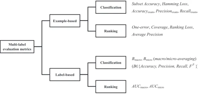
Multi-label evaluation metrics
Example-based
Classification Subset Accuracy, Hamming Loss,
Accuracyexam, Precisionexam, Recallexam, Fexam
Ranking
One-error, Coverage, Ranking Loss,
Average Precision
Label-based
Classification
Bmacro, Bmicro (macro/micro-averaging)
(B {Accuracy, Precision, Recall, F })
Ranking AUCmacro, AUCmicro
β
β
Fig. 1. Summary of major multi-label evaluation metrics.
Note that with respect to h(·), the learning system’s generalization performance is measured from classification perspective. However, for either example-based or label-based metrics, with
respect to the real-valued functionf(·,·)which is returned by most multi-label learning systems as a common practice, the generalization performance can also be measured from ranking
perspective. Fig. 1 summarizes the major multi-label evaluation metrics to be introduced next.
2) Example-based Metrics: Following the notations in Table I, six example-based
classifica-tion metrics can be defined based on the multi-label classifier h(·) [33], [34], [75]:
• Subset Accuracy: subsetacc(h) = 1 p p X i=1 [[h(xi) =Yi]]
The subset accuracy evaluates the fraction of correctly classified examples, i.e. the predicted
label set is identical to the ground-truth label set. Intuitively, subset accuracy can be regarded
as a multi-label counterpart of the traditional accuracy metric, and tends to be overly strict
especially when the size of label space (i.e. q) is large.
• Hamming Loss: hloss(h) = 1 p p X i=1 |h(xi)∆Yi|
Here, ∆stands for the symmetric difference between two sets. The hamming loss evaluates the fraction of misclassified instance-label pairs, i.e. a relevant label is missed or an irrelevant
is predicted. Note that when each example inS is associated with only one label,hlossS(h)
will be 2/q times of the traditional misclassification rate.
• Accuracyexam, Precisionexam, Recallexam, Fβexam:
Accuracyexam(h) = 1 p p X i=1 |YiT h(xi)| |YiS h(xi)|; P recisionexam(h) = 1 p p X i=1 |YiT h(xi)| |h(xi)| Recallexam(h) = 1 p p X i=1 |YiT h(xi)| |Yi| ; F β exam(h) = (1 +β2)·P recision
exam(h)·Recallexam(h)
β2·P recision
exam(h) +Recallexam(h)
Furthermore, Fβ
exam is an integrated version of P recisionexam(h) and Recallexam(h) with
balancing factor β > 0. The most common choice is β = 1 which leads to the harmonic mean of precision and recall.
When the intermediate real-valued function f(·,·) is available, four example-based ranking metrics can be defined as well [75]:
• One-error: one-error(f) = 1 p p X i=1
[[[arg maxy∈Yf(xi, y)]∈/ Yi]]
The one-error evaluates the fraction of examples whose top-ranked label is not in the relevant
label set. • Coverage: coverage(f) = 1 p p X i=1
maxy∈Yirankf(xi, y)−1
The coverage evaluates how many steps are needed, on average, to move down the ranked
label list so as to cover all the relevant labels of the example.
• Ranking Loss: rloss(f) = 1 p p X i=1 1 |Yi||Yi¯||{(y ′, y′′)|f(xi, y′)≤f(xi, y′′), (y′, y′′)∈Yi×Yi¯)}|
The ranking loss evaluates the fraction of reversely ordered label pairs, i.e. an irrelevant
• Average Precision: avgprec(f) = 1 p p X i=1 1 |Yi| X y∈Yi |{y′ |rankf(x,y′)≤ rankf(xi, y), y′ ∈Yi}| rankf(xi, y)
The average precision evaluates the average fraction of relevant labels ranked higher than
a particular label y ∈Yi.
Forone-error, coverage and ranking loss, the smaller the metric value the better the system’s
performance, with optimal value of 1pPpi=1|Yi| −1forcoverageand 0 forone-errorand ranking loss. For the other example-based multi-label metrics, the larger the metric value the better the
system’s performance, with optimal value of 1.
3) Label-based Metrics: For the j-th class label yj, four basic quantities characterizing the binary classification performance on this label can be defined based on h(·):
T Pj =|{xi |yj ∈Yi∧yj ∈h(xi),1≤i≤p}|; F Pj =|{xi |yj ∈/ Yi∧yj ∈h(xi),1≤i≤p}| T Nj =|{xi |yj ∈/ Yi∧yj ∈/ h(xi),1≤i≤p}|; F Nj =|{xi |yj ∈Yi∧yj ∈/h(xi),1≤i≤p}| In other words,T Pj,F Pj,T Nj andF Nj represent the number oftrue positive,false positive,true negative, andfalse negative test examples with respect toyj. According to the above definitions, T Pj +F Pj +T Nj +F Nj =p naturally holds.
Based on the above four quantities, most of the binary classification metrics can be derived
accordingly. Let B(T Pj, F Pj, T Nj, F Nj) represent some specific binary classification metric (B ∈ {Accuracy, P recision, Recall, Fβ}4), the label-based classification metrics can be
ob-tained in either of the following modes [94]:
• Macro-averaging: Bmacro(h) = 1 q q X j=1 B(T Pj, F Pj, T Nj, F Nj) • Micro-averaging: Bmicro(h) =B q X j=1 T Pj, q X j=1 F Pj, q X j=1 T Nj, q X j=1 F Nj ! 4
For example,Accuracy(T Pj, F Pj, T Nj, F Nj) =
T Pj+T Nj T Pj+F Pj+T Nj+F Nj, P recision(T Pj, F Pj, T Nj, F Nj) = T Pj T Pj+F Pj, Recall(T Pj, F Pj, T Nj, F Nj) = T Pj T Pj+F Nj, and F β(T P j, F Pj, T Nj, F Nj) = (1+ β2)·T Pj (1+β2)·T Pj+β2·F Nj+F Pj.
Conceptually speaking, macro-averaging and micro-averaging assume “equal weights” for
labels and examples respectively. It is not difficult to show that both Accuracymacro(h) =
Accuracymicro(h) and Accuracymicro(h) + hloss(h) = 1 hold. Note that the
macro/micro-averaged version (Bmacro/Bmicro) is different to the example-based version in Subsection II-B2.
When the intermediate real-valued functionf(·,·)is available, one label-based ranking metric, i.e. macro-averaged AUC, can be derived as:
AUCmacro = 1 q q X j=1 AUCj = 1 q q X j=1 |{(x′,x′′)|f(x′, yj)≥f(x′′, yj), (x′,x′′)∈ Zj×Z¯j}| |Zj||Z¯j| (2)
Here, Zj = {xi | yj ∈ Yi,1 ≤ i ≤ p} Z¯j ={xi |yj ∈/ Yi,1≤i≤p}
corresponds to the set
of test instances with (without) label yj. The second line of Eq.(2) follows from the close relation between AUC and the Wilcoxon-Mann-Whitney statistic [39]. Correspondingly, the
micro-averaged AUC can also be derived as:
AUCmicro =
|{(x′,x′′, y′, y′′)|f(x′, y′)≥f(x′′, y′′), (x′, y′)∈ S+, (x′′, y′′)∈ S−}|
|S+||S−|
Here, S+ = {(xi, y) | y ∈ Yi,1 ≤ i ≤ p} (S− ={(xi, y)|y /∈Yi,1≤i≤p}) corresponds to
the set of relevant (irrelevant) instance-label pairs.
For the above label-based multi-label metrics, the larger the metric value the better the system’s
performance, with optimal value of 1.
4) Theoretical Results: Based on the metric definitions, it is obvious that existing multi-label
metrics consider the performance from diverse aspects and are thus of different natures. As
shown in Section III, most multi-label learning algorithms actually learn from training examples
by explicitly or implicitly optimizing one specific metric. In light of fair and honest evaluation,
performance of the multi-label learning algorithm should therefore be tested on a broad range of
metrics instead of only on the one being optimized. Specifically, recent theoretical studies show
that classifiers aim at maximizing the subset accuracy would perform rather poor if evaluated
in terms of hamming loss, and vice versa [22], [23].
As multi-label metrics are usually non-convex and discontinuous, in practice most learning
algorithms resort to optimizing (convex) surrogate multi-label metrics [65], [66]. Recently, the
learned classifier converges to the Bayes loss as the training set size increases. Specifically, a
necessary and sufficient condition for consistency of multi-label learning based on surrogate loss
functions is given, which is intuitive and can be informally stated as that for a fixed distribution
overX ×2Y, the set of classifiers yielding optimal surrogate loss must fall in the set of classifiers
yielding optimal original multi-label loss.
By focusing on ranking loss, it is disclosed that none pairwise convex surrogate loss defined
on label pairs is consistent with the ranking loss and some recent multi-label approach [40] is
inconsistent even for deterministic multi-label learning [32].5 Interestingly, in contrast to this negative result, a complementary positive result on consistent multi-label learning is reported
for ranking loss minimization [21]. By using a reduction to the bipartite ranking problem [55],
simple univariate convex surrogate loss (exponential or logistic) defined on single labels is shown
to be consistent with the ranking loss with explicit regret bounds and convergence rates.
III. LEARNING ALGORITHMS
A. Simple Categorization
Algorithm development always stands as the core issue of machine learning researches, with
multi-label learning being no exception. During the past decade, significant amount of algorithms
have been proposed to learning from multi-label data. Considering that it is infeasible to go
through all existing algorithms within limited space, in this review we opt for scrutinizing a
total of eight representative multi-label learning algorithms. Here, therepresentativenessof those
selected algorithms are maintained with respect to the following criteria: a) Broad spectrum:
each algorithm has unique characteristics covering a variety of algorithmic design strategies; b)
Primitive impact: most algorithms lead to a number of follow-up or related methods along its
line of research; and c) Favorable influence: each algorithm is among the highly-cited works in
the multi-label learning field.6
5Here, deterministic multi-label learning corresponds to the easier learning case where for any instance
x∈ X, there exists a label subsetY ⊆ Ysuch that the posteriori probability of observingY givenxis greater than 0.5, i.e.P(Y |x)>0.5.
6
According to Google Scholar statistics (by January 2013), each paper for the eight algorithms has received at least 90 citations, with more than 200 citations on average.
As we try to keep the selection less biased with the above criteria, one should notice that the
eight algorithms to be detailed by no means exclude the importance of other methods.
Further-more, for the sake of notational consistency and mathematical rigor, we have chosen to rephrase
and present each algorithm under common notations. In this paper, a simple categorization of
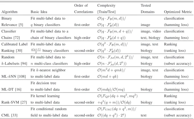
multi-label learning algorithms is adopted [95]:
Problem transformation methods: This category of algorithms tackle multi-label learning
prob-lem by transforming it into other well-established learning scenarios. Representative algorithms
include first-order approaches Binary Relevance [5] and high-order approach Classifier Chains
[72] which transform the task of multi-label learning into the task of binary classification,
second-order approach Calibrated Label Ranking [30] which transforms the task of multi-label learning
into the task of label ranking, and high-order approach Randomk-labelsets [94] which transforms the task of multi-label learning into the task of multi-class classification.
Algorithm adaptation methods: This category of algorithms tackle multi-label learning
prob-lem by adapting popular learning techniques to deal with multi-label data directly.
Repre-sentative algorithms include first-order approach ML-kNN [108] adapting lazy learning tech-niques, first-order approach ML-DT [16] adapting decision tree techtech-niques, second-order
ap-proach Rank-SVM [27] adapting kernel techniques, and second-order apap-proach CML [33]
adapt-ing information-theoretic techniques.
Briefly, the key philosophy of problem transformation methods is to fit data to algorithm,
while the key philosophy of algorithm adaptation methods is to fit algorithm to data. Fig. 2
summarizes the above-mentioned algorithms to be detailed in the rest of this section.
B. Problem Transformation Methods
1) Binary Relevance: The basic idea of this algorithm is to decompose the multi-label learn-ing problem into q independent binary classification problems, where each binary classification problem corresponds to a possible label in the label space [5].
Multi-label learning algorithms Problem transformation Transform to binary classification
Binary Relevance[Subsection III-B.1]
Classifier Chains[Subsection III-B.2]
Transform to label ranking
Calibrated Label Ranking [Subsection III-B.3] Transform to multi-class classification classification Random k-labelsets [Subsection III-B.4] Algorithm adaptation
Lazy learning ML-kNN[Subsection III-C.1]
Decision tree ML-DT[Subsection III-C.2]
Kernel learning Rank-SVM[Subsection III-C.3]
Information-theoretic CML[Subsection III-C.4]
Fig. 2. Categorization of representative multi-label learning algorithms being reviewed.
a corresponding binarytraining set by considering the relevance of each training example to yj:
Dj ={(xi, φ(Yi, yj))|1≤i≤m} (3) where φ(Yi, yj) = +1, if yj ∈Yi −1, otherwise
After that, some binary learning algorithmB is utilized to induce a binary classifiergj :X → R,
i.e. gj ← B(Dj). Therefore, for any multi-label training example (xi, Yi), instance xi will be involved in the learning process ofq binary classifiers. For relevant labelyj ∈Yi, xi is regarded as one positive instance in inducing gj(·); On the other hand, for irrelevant labelyk ∈Yi¯, xi is regarded as one negativeinstance. The above training strategy is termed ascross-trainingin [5].
For unseen instance x, Binary Relevance predicts its associated label set Y by querying labeling relevance on each individual binary classifier and then combing relevant labels:
Y ={yj |gj(x)>0, 1≤j ≤q} (4)
Y=BinaryRelevance(D,B,x)
1. forj= 1toq do
2. Construct the binary training setDj according to Eq.(3);
3. gj← B(Dj);
4. endfor
5. ReturnY according to Eq.(5);
Fig. 3. Pseudo-code of Binary Relevance.
be empty. To avoid producing empty prediction, the following T-Criterion rule can be applied:
Y ={yj |gj(x)>0, 1≤j ≤q} [{yj∗ |j∗ = arg max1≤j≤q gj(x)} (5) Briefly, when none of the binary classifiers yield positive predictions, T-Criterion rule
comple-ments Eq.(4) by including the class label with greatest (least negative) output. In addition to
T-Criterion, some other rules toward label set prediction based on the outputs of each binary
classifier can be found in [5].
Remarks: The pseudo-code of Binary Relevance is summarized in Fig. 3. It is a first-order approach which builds classifiers for each label separately and offers the natural opportunity for
parallel implementation. The most prominent advantage of Binary Relevance lies in its extremely
straightforward way of handling multi-label data (Steps 1-4), which has been employed as the
building block of many state-of-the-art multi-label learning techniques [20], [34], [72], [106].
On the other hand, Binary Relevance completely ignores potential correlations among labels,
and the binary classifier for each label may suffer from the issue of class-imbalance when q is large and label density (i.e. LDen(D)) is low. As shown in Fig. 3, Binary Relevance has computational complexity of O(q· FB(m, d)) for training and O(q· FB′(d)) for testing.7
2) Classifier Chains: The basic idea of this algorithm is to transform the multi-label learning problem into a chain of binary classification problems, where subsequent binary classifiers in
the chain is built upon the predictions of preceding ones [72], [73].
7In this paper, computational complexity is mainly examined with respect to three factors which are common for all learning
algorithms, i.e.:m(number of training examples),d(dimensionality) andq(number of possible class labels). Furthermore, for binary (multi-class) learning algorithmB(M) embedded in problem transformation methods, we denote its training complexity asFB(m, d)(FM(m, d, q)) and its (per-instance) testing complexity asFB′(d)(FM′ (d, q)). All computational complexity results
For q possible class labels {y1, y2,· · ·, yq}, let τ :{1,· · ·, q} → {1,· · ·, q} be a permutation
function which is used to specify an ordering over them, i.e.yτ(1) ≻yτ(2)≻ · · · ≻yτ(q). For the
j-th label yτ(j) (1≤j ≤q)in the ordered list, a corresponding binary training set is constructed
by appending each instance with its relevance to those labels preceding yτ(j):
Dτ(j)={ [xi,preτi(j)], φ(Yi, yτ(j))
|1≤i≤m} (6)
where preiτ(j)= (φ(Yi, yτ(1)),· · ·, φ(Yi, yτ(j−1)))⊤
Here, [xi,preiτ(j)] concatenates vectorsxi andpreiτ(j), andpre
i
τ(j) represents the binary
assign-ment of those labels preceding yτ(j) on xi (specifically, preiτ(1) =∅).8 After that, some binary learning algorithm B is utilized to induce a binary classifier gτ(j) :X × {−1,+1}j−1 →R, i.e.
gτ(j) ← B(Dτ(j)). In other words, gτ(j)(·) determines whether yτ(j) is a relevant label or not.
For unseen instance x, its associated label setY is predicted by traversing the classifier chain iteratively. Let λx
τ(j) ∈ {−1,+1}represent the predicted binary assignment of yτ(j) on x, which
are recursively derived as follows:
λx τ(1) = sign gτ(1)(x) (7) λx τ(j) = sign gτ(j)([x, λxτ(1),· · ·, λ x τ(j−1)]) (2≤j ≤q)
Here, sign[·] is the signed function. Accordingly, the predicted label set corresponds to:
Y ={yτ(j) |λxτ(j) = +1, 1≤j ≤q} (8)
It is obvious that for the classifier chain obtained as above, its effectiveness is largely affected
by the ordering specified by τ. To account for the effect of ordering, an Ensemble of Classifier Chains can be built with n random permutations over the label space, i.e. τ(1), τ(2),· · ·, τ(n).
For each permutation τ(r) (1 ≤ r ≤ n), instead of inducing one classifier chain by applying
τ(r) directly on the original training set D, a modified training set D(r) is used by sampling D
without replacement (|D(r)|= 0.67· |D|) [72] or with replacement (|D(r)|=|D|) [73].
8
In Classifier Chains [72], [73], binary assignment is represented by 0 and 1. Without loss of generality, binary assignment is represented by -1 and +1 in this paper for notational consistency.
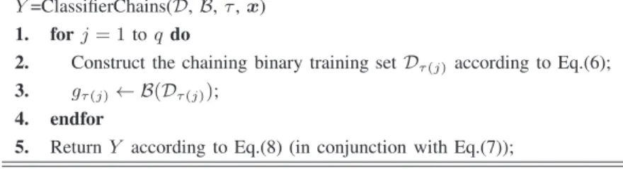
Y=ClassifierChains(D, B,τ,x)
1. forj= 1toq do
2. Construct the chaining binary training setDτ(j) according to Eq.(6);
3. gτ(j)← B(Dτ(j));
4. endfor
5. ReturnY according to Eq.(8) (in conjunction with Eq.(7)); Fig. 4. Pseudo-code of Classifier Chains.
Remarks: The pseudo-code of Classifier Chains is summarized in Fig. 4. It is a high-order
approach which considers correlations among labels in a random manner. Compared to Binary
Relevance [5], Classifier Chains has the advantage of exploiting label correlations while loses the
opportunity of parallel implementation due to its chaining property. During the training phase,
Classifier Chains augments instance space with extra features from ground-truth labeling (i.e.
prei
τ(j) in Eq.(6)). Instead of keeping extra features binary-valued, another possibility is to set
them to the classifier’s probabilistic outputs when the model returned byB (e.g. Naive Bayes) is capable of yielding posteriori probability [20], [105]. As shown in Fig. 4, Classifier Chains has
computational complexity of O(q· FB(m, d+q)) for training and O(q· FB′(d+q)) for testing.
3) Calibrated Label Ranking: The basic idea of this algorithm is to transform the multi-label learning problem into the label ranking problem, where ranking among labels is fulfilled
by techniques of pairwise comparison [30].
For q possible class labels {y1, y2,· · ·, yq}, a total of q(q −1)/2 binary classifiers can be
generated by pairwise comparison, one for each label pair (yj, yk) (1≤j < k ≤q). Concretely, for each label pair(yj, yk), pairwise comparison firstly constructs a corresponding binary training set by considering the relative relevance of each training example to yj and yk:
Djk ={(xi, ψ(Yi, yj, yk))|φ(Yi, yj)6=φ(Yi, yk), 1≤i≤m} (9) where ψ(Yi, yj, yk) =
+1, if φ(Yi, yj) = +1 and φ(Yi, yk) =−1 −1, if φ(Yi, yj) = −1 and φ(Yi, yk) = +1
In other words, only instances with distinct relevance toyj and yk will be included inDjk. After that, some binary learning algorithm B is utilized to induce a binary classifier gjk : X → R,
i.e. gjk ← B(Djk). Therefore, for any multi-label training example (xi, Yi), instance xi will be involved in the learning process of |Yi||Yi¯| binary classifiers. For any instance x ∈ X, the
learning system votes for yj if gjk(x)>0 and yk otherwise.
For unseen instance x, Calibrated Label Ranking firstly feeds it to the q(q−1)/2 trained binary classifiers to obtain the overall votes on each possible class label:
ζ(x, yj) = Xj−1
k=1[[gkj(x)≤0]] +
Xq
k=j+1[[gjk(x)>0]] (1≤j ≤q) (10)
Based on the above definition, it is not difficult to verify that Pqj=1ζ(x, yj) =q(q−1)/2. Here, labels in Y can be ranked according to their respective votes (ties are broken arbitrarily).
Thereafter, some thresholding function should be further specified to bipartition the list of
ranked labels into relevant and irrelevant label set. To achieve this within the pairwise comparison
framework, Calibrated Label Ranking incorporates a virtual label yV into each multi-label
training example(xi, Yi). Conceptually speaking, the virtual label serves as anartificial splitting point between xi’s relevant and irrelevant labels [6]. In other words, yV is considered to be
ranked lower than yj ∈Yi while ranked higher than yk ∈Yi¯.
In addition to the original q(q−1)/2 binary classifiers, q auxiliary binary classifiers will be induced, one for each new label pair (yj, yV) (1 ≤ j ≤q). Similar to Eq.(9), a binary training
set corresponding to (yj, yV) can be constructed as follows:
DjV={(xi, ϕ(Yi, yj, yV))|1≤i≤m} (11)
where ϕ(Yi, yj, yV) =
+1, if yj ∈Yi −1, otherwise
Based on this, the binary learning algorithm B is utilized to induce a binary classifier corre-sponding to the virtual label gjV : X → R, i.e. gjV ← B(DjV). After that, the overall votes
specified in Eq.(10) will be updated with the newly induced classifiers:
ζ∗(x, yj) =ζ(x, yj) + [[gjV(x)>0]] (1≤j ≤q) (12)
Furthermore, the overall votes on virtual label can be computed as:
ζ∗(x, yV) =
Xq
j=1[[gjV(x)≤0]] (13)
Therefore, the predicted label set for unseen instance x corresponds to:
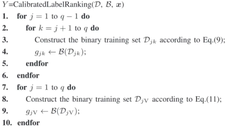
Y=CalibratedLabelRanking(D, B,x)
1. forj= 1toq−1do
2. fork=j+ 1toqdo
3. Construct the binary training setDjk according to Eq.(9);
4. gjk← B(Djk);
5. endfor
6. endfor
7. forj= 1toqdo
8. Construct the binary training setDjV according to Eq.(11);
9. gjV← B(DjV);
10. endfor
11. ReturnY according to Eq.(14) (in conjunction with Eqs.(10)-(13)); Fig. 5. Pseudo-code of Calibrated Label Ranking.
By comparing Eq.(11) to Eq.(3), it is obvious that the training set DjV employed by Calibrated
Label Ranking is identical the training set Dj employed by Binary Relevance [5]. Therefore, Calibrated Label Ranking can be regarded as an enriched version of pairwise comparison, where
the routine q(q −1)/2 binary classifiers are enlarged with the q binary classifiers of Binary Relevance to facilitate learning [30].
Remarks: The pseudo-code of Calibrated Label Ranking is summarized in Fig. 5. It is
a second-order approach which builds classifiers for any pair of class labels. Compared to
previously introduced algorithms [5], [72] which construct binary classifiers in a one-vs-rest
manner, Calibrated Label Ranking constructs binary classifiers (except those for virtual label)
in a one-vs-one manner and thus has the advantage of mitigating the negative influence of
the class-imbalance issue. On the other hand, the number of binary classifiers constructed by
Calibrated Label Ranking grows from linear scale toquadratic scalein terms of the number class
labels (i.e.q). Improvements on Calibrated Label Ranking mostly focus on reducing the quadratic number of classifiers to be queried in testing phase by exact pruning [59] or approximate pruning
[60], [61]. By exploiting idiosyncrasy of the underlying binary learning algorithm B, such as dual representation for Perceptron [58], the quadratic number of classifiers can be induced more
efficiently in training phase [57]. As shown in Fig. 5, Calibrated Label Ranking has computational
complexity of O(q2· F
B(m, d)) for training and O(q2· FB′(d)) for testing.
4) Random k-Labelsets: The basic idea of this algorithm is to transform the multi-label learning problem into an ensemble ofmulti-class classificationproblems, where each component
learner in the ensemble targets a random subset ofYupon which a multi-class classifier is induced by the Label Powerset (LP) techniques [92], [94].
LP is a straightforward approach to transforming label learning problem into
multi-class (single-label) multi-classification problem. Let σY : 2Y →Nbe someinjective function mapping
from the power set of Y to natural numbers, and σY−1 be the corresponding inverse function. In the training phase, LP firstly converts the original multi-label training set D into the following multi-class training set by treating every distinct label set appearing in D as a new class:
DY† ={(xi, σY(Yi))|1≤i≤m} (15)
where the set of new classes covered by DY† corresponds to:
ΓDY†={σY(Yi)|1≤i≤m} (16) Obviously, Γ DY† ≤min m,2 |Y|
holds here. After that, some multi-class learning algorithm
M is utilized to induce a multi-class classifier gY† : X → ΓDY†, i.e. g†Y ← MD†Y. Therefore, for any multi-label training example (xi, Yi), instancexi will be re-assigned with the newly mapped single-label σY(Yi) and then participates in multi-class classifier induction.
For unseen instancex, LP predicts its associated label setY by firstly querying the prediction of multi-class classifier and then mapping it back to the power set of Y:
Y =σY−1g†Y(x) (17)
Unfortunately, LP has two major limitations in terms of practical feasibility: a) Incompleteness:
as shown in Eqs.(16) and (17), LP is confined to predict label sets appearing in the training set,
i.e. unable to generalize to those outside {Yi | 1 ≤ i ≤ m}; b) Inefficiency: when Y is large, there might be too many newly mapped classes in ΓDY†, leading to overly high complexity in training g†Y(·) and extremely few training examples for some newly mapped classes.
To keep LP’s simplicity while overcoming its two major drawbacks, Random k-Labelsets chooses to combine ensemble learning [24], [112] with LP to learn from multi-label data. The
key strategy is to invoke LP only on random k-labelsets (size-k subset in Y) to guarantee computational efficiency, and then ensemble a number of LP classifiers to achieve predictive
Let Yk represent the collection of all possible k-labelsets in Y, where the l-th k-labelset is denoted as Yk(l), i.e. Yk(l) ⊆ Y, Yk(l) = k, 1 ≤ l ≤ qk
. Similar to Eq.(15), a multi-class
training set can be constructed as well by shrinking the original label space Y into Yk(l): DY†k(l) =
xi, σYk(l)(Yi∩ Yk(l)) 1≤i≤m (18) where the set of new classes covered by DY†k(l) corresponds to:
ΓDY†k(l)
={σYk(l)(Yi∩ Yk(l))|1≤i≤m}
After that, the multi-class learning algorithm M is utilized to induce a multi-class classifier gY†k(l) :X →Γ D†Yk(l) , i.e. gY†k(l) ← M D†Yk(l) .
To create an ensemble with n component classifiers, Random k-Labelsets invokes LP on n random k-labelsets Yk(lr) (1 ≤ r ≤ n) each leading to a multi-class classifier g†
Yk(l
r)(·). For
unseen instance x, the following two quantities are calculated for each class label:
τ(x, yj) = Xn r=1[[yj ∈ Y k(lr)]] (1≤j ≤q) (19) µ(x, yj) = Xn r=1 hh yj ∈σ−1 Yk(l r) gY†k(l r)(x) ii (1≤j ≤q)
Here, τ(x, yj) counts themaximum number of votes that yj can be received from the ensemble, whileµ(x, yj)counts theactualnumber of votes thatyj receives from the ensemble. Accordingly, the predicted label set corresponds to:
Y ={yj |µ(x, yj)/τ(x, yj)>0.5, 1≤j ≤q} (20) In other words, when the actual number of votes exceedshalf of the maximum number of votes, yj is regarded to be relevant. For an ensemble created by n k-labelsets, the maximum number of votes on each label is nk/q on average. A rule-of-thumb setting for Random k-Labelsets is k = 3 and n= 2q [92], [94].
Remarks: The pseudo-code of Random k-Labelsets is summarized in Fig. 6. It is a high-order approach where the degree of label correlations is controlled by the size of k-labelsets. In addition to use k-labelset, another way to improve LP is to prune distinct label set in
D appearing less than a pre-specified counting threshold [71]. Although Random k-Labelsets embeds ensemble learning as itsinherentpart to amend LP’s major drawbacks, ensemble learning
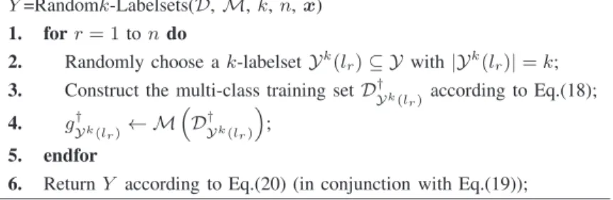
Y=Randomk-Labelsets(D,M,k,n,x)
1. forr= 1tondo
2. Randomly choose ak-labelset Yk(l
r)⊆ Ywith|Yk(lr)|=k;
3. Construct the multi-class training set D†
Yk(lr)according to Eq.(18); 4. gY†k(lr)← M D† Yk(lr) ; 5. endfor
6. ReturnY according to Eq.(20) (in conjunction with Eq.(19)); Fig. 6. Pseudo-code of Randomk-Labelsets.
could be employed as a meta-level strategy to facilitate multi-label learning by encompassing
homogeneous [72], [76] or heterogeneous [74], [83] component multi-label learners. As shown
in Fig. 6, Randomk-Labelsets has computational complexity ofO(n· FM(m, d,2k))for training
and O(n· F′
M(d,2k)) for testing.
C. Algorithm Adaptation Methods
1) Multi-Labelk-Nearest Neighbor (ML-kNN): The basic idea of this algorithm is to adapt k-nearest neighbortechniques to deal with multi-label data, where maximum a posteriori (MAP) rule is utilized to make prediction by reasoning with the labeling information embodied in the
neighbors [108].
For unseen instance x, let N(x) represent the set of its k nearest neighbors identified in D. Generally, similarity between instances is measured with the Euclidean distance. For the j-th class label, ML-kNN chooses to calculate the following statistics:
Cj =X
(x∗,Y∗)∈N(x)[[yj ∈Y
∗]]
(21)
Namely, Cj records the number of x’s neighbors with label yj.
Let Hj be the event that x has label yj, and P(Hj |Cj) represents the posterior probability
thatHj holds under the condition thatxhas exactlyCj neighbors with labelyj. Correspondingly,
P(¬Hj |Cj) represents the posterior probability thatHj doesn’t hold under the same condition.
According to the MAP rule, the predicted label set is determined by deciding whetherP(Hj |Cj)
is greater than P(¬Hj |Cj) or not:
Based on Bayes theorem, we have:
P(Hj |Cj) P(¬Hj |Cj) =
P(Hj)·P(Cj |Hj)
P(¬Hj)·P(Cj | ¬Hj) (23)
Here,P(Hj) (P(¬Hj))represents theprior probabilitythatHj holds (doesn’t hold). Furthermore, P(Cj | Hj) (P(Cj | ¬Hj)) represents the likelihood that x has exactly Cj neighbors with label yj whenHj holds (doesn’t hold). As shown in Eqs.(22) and (23), it suffices to estimate the prior probabilities as well as likelihoods for making predictions.
ML-kNN fulfills the above task via the frequency counting strategy. Firstly, the prior proba-bilities are estimated by counting the number training examples associated with each label:
P(Hj) = s+ Pm
i=1[[yj ∈Yi]]
s×2 +m ; P(¬Hj) = 1−P(Hj) (1≤j ≤q) (24) Here, s is a smoothing parameter controlling the effect of uniform prior on the estimation. Generally, s takes the value of 1 resulting in Laplace smoothing.
Secondly, the estimation process for likelihoods is somewhat involved. For thej-th class label yj, ML-kNN maintains two frequency arrays κj and κj˜ each containing k+1 elements:
κj[r] =Xm i=1[[yj ∈Yi]]·[[δj(xi) =r]] (0≤r≤k) (25) ˜ κj[r] =Xm i=1[[yj ∈/ Yi]]·[[δj(xi) =r]] (0≤r≤k) where δj(xi) = X (x∗,Y∗)∈N(x i) [[yj ∈Y∗]]
Here, δj(xi) records the number of xi’s neighbors with label yj. Therefore, κj[r] counts the number of training examples which have label yj and have exactly r neighbors with label yj, while κj˜ [r] counts the number of training examples which don’t have label yj and have exactly r neighbors with label yj. Afterwards, the likelihoods can be estimated based on κj and κj˜ :
P(Cj |Hj) = s+κj[Cj]
s×(k+ 1) +Pkr=0κj[r] (1≤j ≤q, 0≤Cj ≤k) (26) P(Cj | ¬Hj) = s+ ˜κj[Cj]
s×(k+ 1) +Pkr=0˜κj[r] (1≤j ≤q, 0≤Cj ≤k)
Thereafter, by substituting Eq.(24) (prior probabilities) and Eq.(26) (likelihoods) into Eq.(23),
Y=ML-kNN(D,k,x)
1. fori= 1tomdo
2. Identifyknearest neighborsN(xi)forxi;
3. endfor
4. forj= 1toqdo
5. Estimate the prior probabilitiesP(Hj) andP(¬Hj)according to Eq.(24);
6. Maintain frequency arraysκjand ˜κj according to Eq.(25);
7. endfor
8. Identifyknearest neighborsN(x)forx;
9. forj= 1toqdo
10. Calculate statisticCjaccording to Eq.(21);
11. endfor
12. ReturnY according to Eq.(22) (in conjunction with Eqs.(23), (24) and (26)); Fig. 7. Pseudo-code of ML-kNN.
Remarks:The pseudo-code of ML-kNN is summarized in Fig. 7. It is a first-orderapproach which reasons the relevance of each label separately. ML-kNN has the advantage of inheriting merits of both lazy learning and Bayesian reasoning: a) decision boundary can be adaptively
adjusted due to thevarying neighborsidentified for each unseen instance; b) the class-imbalance
issue can be largely mitigated due to theprior probabilitiesestimated for each class label. There
are other ways to make use of lazy learning for handling multi-label data, such as combining kNN with ranking aggregation [7], [15], identifying kNN in a label-specific style [41], [101], expandingkNN to cover the whole training set [14], [49]. Considering that ML-kNN is ignorant of exploiting label correlations, several extensions have been proposed to provide patches to
ML-kNN along this direction [13], [104]. As shown in Fig. 7, ML-kNN has computational complexity of O(m2d+qmk) for training and O(md+qk) for testing.
2) Multi-Label Decision Tree (ML-DT): The basic idea of this algorithm is to adoptdecision treetechniques to deal with label data, where an information gain criterion based on
multi-label entropy is utilized to build the decision tree recursively [16].
Given any multi-label data set T ={(xi, Yi)| 1≤i ≤n} with n examples, the information gain achieved by dividing T along the l-th feature at splitting value ϑ is:
IG(T, l, ϑ) = MLEnt(T)−X ρ∈{−,+} |Tρ| |T | ·MLEnt(T ρ ) (27)
Namely, T− (T+) consists of examples with values on the l-th feature less (greater) than ϑ.9
Starting from the root node (i.e.T =D), ML-DT identifies the feature and the corresponding splitting value which maximizes the information gain in Eq.(27), and then generates two child
nodes with respect to T− and T+. The above process is invoked recursively by treating either
T− or T+ as the new root node, and terminates until some stopping criterionC is met (e.g. size
of the child node is less than the pre-specified threshold).
To instantiate ML-DT, the mechanism for computing multi-label entropy, i.e. MLEnt(·) in Eq.(27), needs to be specified. A straightforward solution is to treat each subset Y ⊆ Y as a new class and then resort to the conventional single-label entropy:
\ MLEnt(T) =−X Y⊆Y P(Y)·log 2(P(Y)) (28) where P(Y) = Pn i=1[[Yi =Y]] n
However, as the number of new classes grows exponentially with respect to |Y|, many of them might not even appear inT and thus only have trivial estimated probability (i.e. P(Y) = 0). To
circumvent this issue, ML-DT assumesindependenceamong labels and computes the multi-label
entropy in a decomposable way:
MLEnt(T) =Xq j=1−pjlog2pj−(1−pj) log2(1−pj) (29) where pj = Pn i=1[[yj ∈Yi]] n
Here,pj represents the fraction of examples inT with labelyj. Note that Eq.(29) can be regarded as a simplified version of Eq.(28) under the label independence assumption, and it holds that
MLEnt(T)≥MLEnt(T\ ).
For unseen instance x, it is fed to the learned decision tree by traversing along the paths until
reaching a leaf node affiliated with a number of training examples T ⊆ D. Then, the predicted label set corresponds to:
Y ={yj | pj >0.5, 1≤j ≤q} (30)
9
Without loss of generality, here we assume that features are real-valued and the data set is bi-partitioned by setting splitting point along each feature. Similar to Eq.(27), information gain with respect to discrete-valued features can be defined as well.
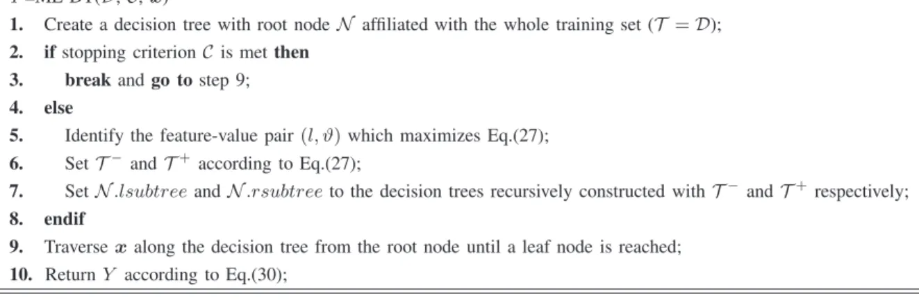
Y=ML-DT(D,C,x)
1. Create a decision tree with root nodeN affiliated with the whole training set (T =D);
2. ifstopping criterionC is metthen
3. breakandgo tostep 9;
4. else
5. Identify the feature-value pair(l, ϑ)which maximizes Eq.(27);
6. SetT−andT+ according to Eq.(27);
7. SetN.lsubtreeandN.rsubtreeto the decision trees recursively constructed withT−andT+respectively;
8. endif
9. Traversexalong the decision tree from the root node until a leaf node is reached;
10. ReturnY according to Eq.(30);
Fig. 8. Pseudo-code of ML-DT.
In other words, if for one leaf node the majority of training examples falling into it have label
yj, any test instance allocated within the same leaf node will regard yj as its relevant label. Remarks: The pseudo-code of ML-DT is summarized in Fig. 8. It is a first-order approach which assumes label independence in calculating multi-label entropy. One prominent advantage
of ML-DT lies in its high efficiency in inducing the decision tree model from multi-label data.
Possible improvements on multi-label decision trees include employing pruning strategy [16]
or ensemble learning techniques [52], [110]. As shown in Fig. 8, ML-DT has computational
complexity of O(mdq)for training and O(mq) for testing.
3) Ranking Support Vector Machine (Rank-SVM): The basic idea of this algorithm is to adapt maximum margin strategy to deal with multi-label data, where a set of linear classifiers
are optimized to minimize the empirical ranking loss and enabled to handle nonlinear cases with
kernel tricks [27].
Let the learning system be composed ofqlinear classifiersW ={(wj, bj)|1≤ j ≤q}, where wj ∈Rd and bj ∈R are theweight vector andbias for thej-th class label yj. Correspondingly, Rank-SVM defines the learning system’s margin on (xi, Yi) by considering its ranking ability on the example’s relevant and irrelevant labels:
min
(yj,yk)∈Yi×Y¯i
hwj −wk,xii+bj −bk kwj −wkk
(31)
Here, hu,vireturns the inner product u⊤v. Geometrically speaking, for each relevant-irrelevant label pair(yj, yk)∈Yi×Yi¯, their discrimination boundary corresponds to the hyperplane hwj− wk,xi+bj−bk = 0. Therefore, Eq.(31) considers the signed L2-distance of xi to hyperplanes
of every relevant-irrelevant label pair, and then returns the minimum as the margin on (xi, Yi). Therefore, the learning system’s margin on the whole training set D naturally follows:
min (xi,Yi)∈D min (yj,yk)∈Yi×Y¯i hwj−wk,xii+bj −bk kwj −wkk (32)
When the learning system is capable of properly ranking every relevant-irrelevant label pair for
each training example, Eq.(32) will returnpositive margin. In this ideal case, we can rescale the
linear classifiers to ensure: a) ∀ 1≤i≤m and (yj, yk)∈Yi×Yi,¯ hwj−wk,xii+bj−bk >1; b) ∃ i∗ ∈ {1,· · ·, m} and (yj
∗, yk∗)∈ Yi∗ ×Yi¯∗, hwj∗−wk∗,xi∗i+bj∗ −bk∗ = 1. Thereafter, the problem of maximizing the margin in Eq.(32) can be expressed as:
max W (ximin,Yi)∈D min (yj,yk)∈Yi×Y¯i 1 kwj−wkk2 (33) subject to : hwj−wk,xii+bj−bk≥1 (1 ≤i≤m, (yj, yk)∈Yi×Yi¯)
Suppose we have sufficient training examples such that for each label pair(yj, yk) (j 6=k), there exists(x, Y)∈ Dsatisfying(yj, yk)∈Y ×Y¯. Thus, the objective in Eq.(33) becomes equivalent to maxWmin1≤j<k≤qkw 1
j−wkk2 and the optimization problem can be re-written as: min
W 1≤maxj<k≤qkwj−wkk
2 (34)
subject to : hwj−wk,xii+bj−bk≥1 (1 ≤i≤m, (yj, yk)∈Yi×Yi¯)
To overcome the difficulty brought by themaxoperator, Rank-SVM chooses to simplify Eq.(34) by approximating the max operator with the sum operator:
min W Xq j=1kwjk 2 (35) subject to : hwj−wk,xii+bj−bk≥1 (1 ≤i≤m, (yj, yk)∈Yi×Yi¯)
To accommodate real-world scenarios where constraints in Eq.(35) can not be fully satisfied,
slack variables can be incorporated into Eq.(35):
min {W,Ξ} Xq j=1kwjk 2+CXm i=1 1 |Yi||Yi¯| X (yj,yk)∈Yi×Y¯i ξijk (36) subject to : hwj −wk,xii+bj−bk ≥1−ξijk ξijk ≥0 (1≤i≤m, (yj, yk)∈Yi×Yi¯)
Y=Rank-SVM(D,C,x)
1. Induce the classification systemW={(wj, bj)|1≤j≤q}by solving the QP problem in Eq.(36);
2. Induce(w∗, b∗)for the thresholding function by solving the linear least square problem in Eq.(1);
3. ReturnY according to Eq.(37);
Fig. 9. Pseudo-code of Rank-SVM.
Here, Ξ = {ξijk | 1 ≤ i ≤ m, (yj, yk) ∈ Yi ×Yi¯} is the set of slack variables. The objective in Eq.(36) consists of two parts balanced by the trade-off parameter C. Specifically, the first part corresponds to themargin of the learning system, while the second parts corresponds to the
surrogate ranking loss of the learning system implemented in hinge form. Note that surrogate
ranking loss can be implemented in other ways such as the exponential form for neural network’s
global error function [107].
Note that Eq.(36) is a standard quadratic programming (QP) problem with convex objective
and linear constraints, which can be tackled with any off-the-shelf QP solver. Furthermore, to
endow Rank-SVM with nonlinear classification ability, one popular way is to solve Eq.(36) in
its dual form via kernel trick. More details on the dual formulation can be found in [26].
As discussed in Subsection II-A3, Rank-SVM employs the stacking-style procedure to set the
thresholding function t(·), i.e. t(x) =hw∗,f∗(x)i+b∗ with f∗(x) = (f(x, y
1),· · ·, f(x, yq))T
and f(x, yj) = hwj,xi+bj. For unseen instancex, the predicted label set corresponds to: Y ={yj | hwj,xi+bj >hw∗,f∗(x)i+b∗, 1≤j ≤q} (37) Remarks: The pseudo-code of Rank-SVM is summarized in Fig. 9. It is a second-order approach which defines the margin over hyperplanes for relevant-irrelevant label pairs.
Rank-SVM benefits from kernels to handle nonlinear classification problems, and further variants can
be achieved. Firstly, as shown in [37], the empirical ranking loss considered in Eq.(40) can
be replaced with other loss structures such as hamming loss, which can be cast as a general
form of structured output classification [86], [87]. Secondly, the thresholding strategy can be
accomplished with techniques other than stacking-style procedure [48]. Thirdly, to avoid the
problem of kernel selection, multiple kernel learning techniques can be employed to learn from
multi-label data [8], [46], [81]. As shown in Fig. 9, let FQP(a, b) represent the time complexity
complexity of O(FQP(dq+mq2, mq2) +q2(q+m))for training and O(dq) for testing.
4) Collective Multi-Label Classifier (CML): The basic idea of this algorithm is to adapt maximum entropy principle to deal with multi-label data, where correlations among labels are
encoded as constraints that the resulting distribution must satisfy [33].
For any multi-label example (x, Y), let (x,y) be the corresponding random variables repre-sentation using binary label vector y = (y1, y2,· · ·, yq)⊤ ∈ {−1,+1}q, whose j-th component
indicates whether Y contains the j-th label (yj = +1) or not (yj =−1). Statistically speaking, the task of multi-label learning is equivalent to learn a joint probability distribution p(x,y).
Let Hp(x,y) represent the information entropy of (x,y) given their distribution p(·,·). The principle of maximum entropy [45] assumes that the distribution best modeling the current state
of knowledge is the one maximizing Hp(x,y)subject to a collection K of given facts: max
p Hp(x,y) (38)
subject to : Ep[fk(x,y)] =Fk (k ∈ K)
Generally, the fact is expressed as constraint on the expectation of some function over (x,y), i.e. by imposingEp[fk(x,y)] =Fk. Here,Ep[·]is the expectation operator with respect top(·,·),
whileFkcorresponds to the expected value estimated from training set, e.g. m1 P
(x,y)∈Dfk(x,y).
Together with the normalization constraint on p(·,·) (i.e. Ep[1] = 1), the constrained
opti-mization problem of Eq.(38) can be carried out with standard Lagrange Multiplier techniques.
Accordingly, the optimal solution is shown to fall within the Gibbs distribution family [1]:
p(y|x) = 1 ZΛ(x) expX k∈Kλk·fk(x,y) (39)
Here, Λ ={λk |k ∈ K} is the set of parameters to be determined, and ZΛ(x) is the partition
function serving as the normalization factor, i.e. ZΛ(x) =Pyexp
P
k∈Kλk·fk(x,y)
.
By assuming Gaussian prior (i.e.λk ∼ N(0, ε2)), parameters inΛcan be found by maximizing
the following log-posterior probability function:
l(Λ| D) = log Y (x,y)∈Dp(y|x) −X k∈K λ2 k 2ε2 (40) = X (x,y)∈D X k∈Kλk·fk(x,y)−logZΛ(x) −X k∈K λ2 k 2ε2