On the Value of User Preferences in Search-Based Software Engineering: A Case Study in Software Product Lines

On the Value of User Preferences in Search-Based

Software Engineering: A Case Study in Software

Product Lines

Abdel Salam Sayyad

Tim Menzies

Hany Ammar

Lane Department of Computer Science and Electrical Engineering West Virginia University

Morgantown, WV, USA

asayyad@mix.wvu.edu tim@menzies.us hany.ammar@mail.wvu.edu

Abstract—Software design is a process of trading off competing objectives. If the user objective space is rich, then we should use optimizers that can fully exploit that richness. For example, this study configures software product lines (expressed as feature maps) using various search-based software engineering methods. As we increase the number of optimization objectives, we find that methods in widespread use (e.g. NSGA-II, SPEA2) perform much worse than IBEA (Indicator-Based Evolutionary Algorithm). IBEA works best since it makes most use of user preference knowledge. Hence it does better on the standard measures (hypervolume and spread) but it also generates far more products with 0% violations of domain constraints. Our conclusion is that we need to change our methods for search-based software engineering, particularly when studying complex decision spaces.

Index Terms—Software Product Lines, Feature Models, Optimal Feature Selection, Multiobjective Optimization, Indicator-Based Evolutionary Algorithm, Search-Based Software Engineering.

I. INTRODUCTION

As software changes from product-based to app-based, this changes the nature of software engineering. Previously, in product-based methods, vendors tried to retain their user base via some complete solution to all their anticipated needs (e.g. Microsoft Office). Such large software platforms are very complex and, hence, very slow to change.

With smart phones and tablet-based software, users can choose from large numbers of small apps from different vendors, each performing a specific small task. In app-based software engineering, vendors must quickly and continually reconfigure their apps in order to retain and extend their customer base. This new style of software engineering demands a new style of feature-based analysis. For example, feature maps are a lightweight method for defining a space of options as well as assessing the value of a particular subset of those options.

Feature models allow visualization, reasoning, and configuration of large and complex software product lines (SPLs). Common SPLs now consist of hundreds (even thousands) of features, with complex dependencies and constraints that govern which features can or cannot live and interact with other features. For instance, according to [3], the Linux model has 6320 features, of which 86% declare constraints of some sort, and most features refer to 2-4 other

features. Such level of complexity surely requires automated reasoning and configuration techniques, especially if the intricacies of the feature model are combined with further user preferences and priorities, such as those related to cost and reliability. In that case, the job of offering product variants with guaranteed conformance to the feature model and efficiency according to user preferences becomes monumental, requiring tool assistance.

The automation of optimal feature selection in SPLs has been attempted before, but never with multiobjective evolutionary optimization algorithms (MEOAs). Previous approaches will be highlighted in section II.

The logical structure of feature models poses a challenge to evolutionary techniques, since those techniques depend on random crossover and mutation which invariably destroy feature dependencies and constraints. In [12], this hurdle is overcome by introducing a repair operator to “surgically” make each candidate solution fully-compatible with the feature model after each round of crossover and mutation. In our opinion, this approach fails to take advantage of the automatic correction afforded by the metaheuristic algorithms via “survival of the fittest”. As we show in this paper, conformance with the feature model can be achieved by the evolutionary algorithms (especially IBEA) without resorting to a repair operator or special crossover and mutation operators. We demonstrate how logical correctness can be obtained by generating a range of solutions (i.e. a Pareto front) which include fully-correct and marginally-incorrect solutions (solutions with a very small number of rule violations), as well as totally intolerable ones. We believe that by shedding light on marginally-incorrect solutions we provide wider configuration options to product managers, and might inspire software developers to rethink the feature model and the relationships defined therein.

More importantly, the main contribution of this paper is true, high-dimensional multiobjective search, which puts each user preference in focus without aggregation, and then incorporates the user preferences in the Pareto dominance criteria, using the Indicator-Bases Evolutionary Algorithm (IBEA). We show remarkable results obtained with IBEA compared to six other multiobjective evolutionary optimization algorithms (MEOAs). Up to 5 optimization objectives are used, namely: to maximize logical (syntactic) correctness, maximize richness of feature offering, minimize cost, maximize code

reuse and minimize known defects. We demonstrate how popular algorithms such as NSGA-II and SPEA2 become useless as we increase the number of objectives, a result that was shown in other domains [27] but never before in software engineering.

The uniqueness of IBEA comes from the way it calculates dominance as a value, which incorporates the user preferences (i.e. optimization objectives), thus providing an “amount” of dominance. All other algorithms rank solutions in the objective space according to absolute dominance, with second preference given to diversity of solutions. The glaring superiority of IBEA at higher dimensions shown in this work gives software engineers this take-home message:

“If your user preference space is rich, then use an MEOA that can exploit that richness.”

The rest of the paper is organized as follows: section II reviews related work in automated software product configuration, as well as the use of multiobjective evolutionary optimization algorithms (MEOAs) in software engineering. Section III provides background material on software product lines and MEOAs. Sections IV and V describe the experimental setup and the results of the experiments. In sections VI, we discuss the findings and their implications. Section VII presents the threats to validity. And in the final section, we present our conclusions and future work.

II. RELATED WORK

A. Automated Software Product Configuration

First, we discuss related work in the area of automated product configuration and feature selection.

In our previous work [26], we analyzed feature models using a data mining technique, which runs over thousands of randomly-generated product variants and identifies the most critical feature choices that amount to the most constraint violations. Based on that, we offered recommendations as to where the configuration task should begin in order to avoid related errors. In the present work we augment the feature models with quality attributes and seek to find the optimal product variants based on the desired preferences.

The idea of extending (or augmenting) feature models with quality attributes was proposed by many, among them Zhang et al. [32]. The following papers used a similar approach and synthetic data to experiment with optimizing feature selection in SPLs.

Benavides et al. [1] provided automated reasoning on extended feature models. They assigned extra-functionality such as price range or time range to features. They modeled the problem as a Constraint Satisfaction Problem, and solved it using CSP solvers to return a set of features which satisfy the stakeholders’ criteria.

White et al. [28] mapped the feature selection problem to a multidimensional multi-choice knapsack problem (MMKP). They apply Filtered Cartesian Flattening to provide partially optimal feature configuration.

Also White et al. [29] introduced the MUSCLE tool which provided a formal model for multistep configuration and mapped it to constraint satisfaction problems (CSPs). Hence,

CSP solvers were used to determine the path from the start of the configuration to the desired final configuration. Non-functional requirements were considered such as cost constraints between two configurations. A sequence of minimal feature adaptations is calculated to reach from the initial to the desired feature model configurations.

The limitations of these methods are obvious, given the small models that they experimented with. As SPLs become larger the problem grows more intractable. More recently, a Genetic Algorithm was used to tackle this problem [12]. Although the problem is obviously multiobjective, the various objectives where aggregated into one and a simple GA was used. The result is to provide the product manager with only one “optimal” configuration, which is only optimal according to the weights chosen in the objective formula. Also, they used a repair operator to keep all candidate solutions in line with the feature model all throughout the evolutionary process. We contend with this, as discussed in the introduction.

B. Use of MEOAs in Software Engineering

We now review broadly-related work in the area of multiobjective optimization applied to various problems in Software Engineering.

Historically, the field of Search-Based Software Engineering (SBSE) has seen a slow adoption of MEOAs. Back in 2001, when Harman and Jones coined the term SBSE [14], all surveyed and suggested techniques were based on single-valued fitness functions. In 2007, Harman commented on the current state and future of SBSE [13], and in the “Road-map for Future Work” section he suggested using multiobjective optimization. Then in 2009, Harman et al. [16] were able to cite several works in which multiobjective evolutionary optimization techniques were deployed. Still, most of the work reviewed therein, as well as work done thereafter, optimized two objectives only, while higher numbers appeared only occasionally. Also, the typical tendency was to use algorithms that are popular in other domains, such as NSGA-II and SPEA2. To support these two assertions, Table 1 lists examples of papers that used MEOAs in various software engineering problems, along with number of objectives and the algorithms used.

Among the papers in Table 1, the paper by Bowman et al. [4] is noted for using 5 objectives, and achieving good results with SPEA2. We attribute that to the moderate size of the model, and lack of complexity within. In our experiment, SPEA2 does not perform well with 5 objectives when applied to the relatively large E-Shop feature model.

A literature survey of Pareto-Optimal Search-Based Software Engineering [25] confirms these tendencies after studying 51 related papers. For example, 70% of the papers only applied a single multiobjective algorithm to their problems. Most researchers chose their algorithms based on popularity (especially NSGA-II); often time not stating any reasons for their choice. It also shows that most papers tackled two or three optimization objectives. Very few examples were found where the researchers analyzed the suitability of certain algorithms for the problems at hand. Consequently, the field of SBSE is ripe for much reconsideration of algorithms, reformulation of problems, and performance comparisons.

TABLE 1:EXAMPLES OF USE OF MEOAS IN SOFTWARE ENGINEERING

Reference Application Number of _Objectives MEOA Used

Zhang et al., 2007 [31] Next release problem 2 NSGA-II, Pareto GA

Lakhotia et al., 2007 [15] Test data generation 2 NSGA-II

Yoo and Harman, 2007 [30] Test case selection 2, 3 NSGA-II, vNSGA-II

Gueorguiev et al., 2009 [11] Software project planning for robustness and completion time 2 SPEA2

Bowman et al., 2010 [4] Class responsibility assignment problem 5 SPEA2

Colanzi et al., 2011 [5] Generating integration test orders for aspect-oriented software 2 NSGA-II, SPEA2 Heaven and Letier, 2011 [17] Optimizing design decisions in quantitative goal models 2 NSGA-II

III. BACKGROUND

A. Software Product Line Engineering (SPLE)

Increasingly, software engineers spend their time creating software families consisting of similar systems with many variations [6]. Many researchers in industry and academia started using a feature-oriented approach to commonality and variability analysis after the Software Engineering Institute introduced Feature-Oriented Domain Analysis (FODA) in 1990 [18]. Software product line engineering is a paradigm to develop software applications using platforms and mass customization. Benefits of SPLE include reduction of development costs, enhancement of quality, reduction of time to market, reduction of maintenance effort, coping with evolution and complexity [24], and identifying opportunities for automating the creation of family members [6].

B. Feature Models and the SXFM format

A feature is an end-user-visible behavior of a software product that is of interest to some stakeholder. A feature model represents the information of all possible products of a software product line in terms of features and relationships among them. Feature models are a special type of information model widely used in software product line engineering. A feature model is represented as a hierarchically arranged set of features composed by:

1. Relationships between a parent feature and its child features (or subfeatures).

2. Cross-tree constraints that are typically inclusion or exclusion statements in the form: if feature F is included, then features A and B must also be included (or excluded). Figure 1, adapted from [2], depicts a simplified feature model inspired by the mobile phone industry.

The Simple XML Feature Model (SXFM) format was defined by the SPLOT website [21], which was launched in May 2009. SPLOT is host to a feature model repository which adheres to the SXFM format. Figure 2 shows the SXFM format for the mobile phone feature model from Figure 1. It shows the root feature (marked with :r), the mandatory features (marked with :m), the optional features (marked with :o), and the group features (marked with :g). The cross-tree constraints are listed at the bottom in Conjunctive Normal Form (CNF).

The full set of rules in a feature model can be captured in a Boolean expression, such as the one in Figure 3, which shows the expression for the mobile phone feature model. From it we can conclude that the total number of rules in this feature model is 16, including the following:

 The root feature is mandatory.  Every child requires its own parent.

Figure 1: Feature model for mobile phone product line

Figure 2: Mobile Phone feature model in SXFM format

Figure 3: Mobile phone feature model as a Boolean expression <feature_model name="Mobile-Phone">

<meta>

<data name="description">Mobile Phone</data> … </meta> <feature_tree> :r Mobile Phone(root) :m calls(calls) :o GPS(gps) :m screen(screen) :g (_g_1) [1,1] : basic(basic) : color(color) : high-resolution(hi_res) :o media(media) :g (_g_2) [1,*] : camera(camera) : mp3(mp3) </feature_tree> <constraints> constraint_1: ~gps or ~basic constraint_2: camera or ~hi_res </constraints>

</feature_model>

FM = (Mobile Phone ↔ Calls) ˄ (Mobile Phone ↔ Screen) ˄ (GPS → Mobile Phone) ˄ (Media → Mobile Phone)

˄ (Screen ↔ XOR (Basic, Color, High resolution)) ˄ (Media ↔ Camera ˅ MP3)

˄ (Camera → High resolution) ˄ ¬(GPS ˄ Basic)

 If the child is mandatory, the parent requires the child.

 Every group adds a rule about how many members can be chosen.

 Every cross-tree constraint (CTC) is a rule.

The total number of rules will be used as the “full correctness” score in this experiment, thus making “correctness” one of the optimization objectives.

The feature models used in this study were downloaded from SPLOT, and were further augmented with properties pertaining to cost and reliability to allow for multiobjective optimization, as will be explained in section IV.

C. Multiobjective Evolutionary Optimization Algorithms (MEOAs)

Many real-world problems involve simultaneous optimization of several incommensurable and often competing objectives. Often, there is no single optimal solution, but rather a set of alternative solutions. These solutions are optimal in the wider sense that no other solutions in the search space are superior to them when all objectives are considered [34].

Formally, we define two types of Pareto Dominance:

Boolean Dominance is defined as follows: A vector is said to dominate a vector if and only if u is partially less than v, i.e.

, (1) whereas Continuous Dominance is measured with a continuous function, such as equation 2 in Figure 4.

The Pareto Front is defined as the set of all points in the objective space that are not dominated by any other points.

Many algorithms have been suggested over the past two decades for multiobjective optimization based on evolutionary algorithms that were designed primarily for single-objective optimization, such as Genetic Algorithms, Evolutionary Strategies, Particle Swarm Optimization, and Differential Evolution.

The algorithms we used in this study were already implemented in the jMetal framework [8]. They are:

1- IBEA: Indicator-Based Evolutionary Algorithm [33]. 2- NSGA-II: Nondominated Sorting Genetic Algorithm, version 2 [7].

3- ssNSGA-II, a “steady-state” version of NSGA-II [9]. 4- SPEA2: Strength Pareto Evolutionary Algorithm, version 2 [35].

5- FastPGA: Fast Pareto Genetic Algorithm [10].

6- MOCell: A Cellular Genetic Algorithm for Multiobjective Optimization [23].

7- MOCHC: A Multiobjective version of CHC, which stands for: Cross generational elitist selection, Heterogeneous recombination, Cataclysmic mutation [22].

Table 2 provides a brief comparison among the 7 algorithms, highlighting their major properties.

D. Indicator-Based Evolutionary Algorithm

Of the 7 algorithms listed above, IBEA is unique in terms of its dominance criteria. All other algorithms followed a

ranking approach according to Boolean dominance (equation 1), while favoring diversity in the Pareto-optimal set of solutions. They only gave each solution a place in the ranking. IBEA, on the other hand, makes more use of the preference criteria. Equation 2 in Figure 4 shows IBEA's continuous dominance criteria where each solution is given a weight based on quality indicators, thus factoring in more of the optimization objectives of the user. The authors of IBEA, Zitzler and Kunzli, designed the algorithm such that “preference information of the decision maker” can be “integrated into multiobjective search.” In Figure 4, we provide an outline of the IBEA algorithm. The details can be found in [33].

Figure 4: Outline of IBEA ( ) ∑ ( )

( ) Input: α (population size)

N (maximum number of generations)

κ (fitness scaling factor) Output: A (Pareto set approximation) Step 1: Initialization: Generate an initial

population P of size α; and an initial mating pool

P’ of size α; append P’ to P; set the generation

counter m to 0.

Step 2: Fitness assignment: Calculate fitness values of individuals in P, i.e., for all x1 ∈ P set

Where I(.) is a dominance-preserving binary indicator.

Step 3: Environmental selection: Iterate the following three steps until the size of population

P does not exceed α:

1. Choose an individual x∗ ∈ P with the smallest fitness value, i.e., F(x∗) ≤ F(x) for all x ∈ P. 2. Remove x∗ from the population.

3. Update the fitness values of the remaining individuals, i.e.

F(x) = F(x) + ( ) _{for all x ∈ P.}

Step 4: Termination: If m ≥ N or another stopping criterion is satisfied then set A to the set of decision vectors represented by the nondominated individuals in P. Stop. Step 5: Mating selection: Perform binary tournament selection with replacement on P in order to fill the temporary mating pool P’.

Step 6: Variation: Apply recombination and mutation operators to the mating pool P’ and add the resulting offspring to P. Increment the

TABLE 2:COMPARISON OF MULTIOBJECTIVE EVOLUTIONARY OPTIMIZATION ALGORITHMS

Algorithm Population Operators Domination criteria Goal of domination criteria

IBEA Main +

archive

Crossover, mutation, environmental selection

Calculates domination value (i.e. amount of dominance) based on indicator (e.g. hypervolume). Favors those dominating by far.

Favor objectives, i.e. user preferences

NSGA-II One Crossover, mutation, tournament selection

Calculates distance to closest point for each objective. Fitness is product of these distances. Favors higher fitness, i.e. more isolated points.

Favor absolute domination and more spread out solutions.

ssNSGA-II One Crossover, mutation, tournament selection Same as NSGA-II. But, only one new individual inserted into population at a time. Favor absolute domination and more spread out solutions.

SPEA2 External & internal

Crossover, mutation, tournament selection

Strength of an external point is number of points dominated by it or equal to it. Strength of an internal point is sum of strengths of points dominating or equal. Minimize strength to minimize crowding.

Favor absolute domination and more spread out solutions.

FastPGA One Crossover, mutation, tournament selection, dynamic population sizing

The fitness of the nondominated solutions is calculated using the crowding distance as in NSGA-II. The fitness of dominated solution is the number of solutions it

dominates, similar to SPEA2. Ranking by both domination and fitness.

Favor absolute domination and more spread out solutions. MOCell Main + archive Crossover, mutation, tournament selection, random feedback

The solutions are ordered using a ranking and a crowding distance estimator similar to NSGA-II. Bigger distance values are favored.

Favor absolute domination and more spread out solutions.

MOCHC One Crossover, cataclysmic mutation, ranking & crowding selection

The solutions are ordered using a ranking and a crowding distance estimator similar to NSGA-II. Bigger distance values are favored.

Favor absolute domination and more spread out solutions.

E. Quality of Pareto Front

Quality indicators can be calculated to assess the performance of multiobjective metaheuristics. In this study, we used two indicators:

1- Hypervolume: defined in [34] as a measure of the size of the space covered, as follows: Let (x1, x2, …, xk) be a set of

decision vectors. The hypervolume is the volume enclosed by the union of the polytopes (p1, p2, …, pk) where each pi is

formed by the intersections of the following hyperplanes arising out of xi, along with the axes: for each axis in the

objective space, there exists a hyperplane perpendicular to the axis and passing through the point (f1(xi), f2(xi), …, fn(xi)). In

the two-dimensional (2-D) case, each pi represents a rectangle

defined by the points (0,0) and (f1(xi), f2(xi)). In jMetal, all

objectives are minimized, but the Pareto front is inverted before calculating hypervolume, thus the preferred Pareto front would be that with the most hypervolume.

2- Spread: defined in [7], measures the extent of spread in the obtained solutions. It is found with the formula:

∑ ̅

( ) ̅ ( ) Where:

N is the number of points in the Pareto front,

diis Euclidean distances between consecutive points,

̅ is Average of di’s, and

df and dl are the Euclidean distances between the extreme

solutions and the boundary solutions of the Pareto front. Other quality indicators are used elsewhere, namely: generational distance, inverted generational distance, epsilon, and generalized speed. These indicators weren’t used here

since they compare the calculated Pareto Front to a previously-known “true Pareto Front”, which we do not have in this case.

An indicator that is particular to this problem is the percentage of correct solutions, since correctness is an optimization objective that allows product configurations to evolve into full conformance with the feature model. We are interested in points within the Pareto front that have zero violations, and thus a full-correctness score. The importance of this indicator will become very clear in this experiment.

IV. SETUP

A. Setting Up Feature Models

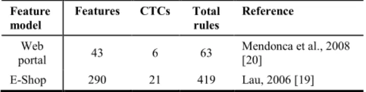
The two feature models used in this study belong to the feature model repository at SPLOT website [21], a popular repository used by many researchers. We chose “Web Portal”, a moderate-size feature model, and “E-Shop”, the largest feature model in that repository. Table 3 shows the feature models, along with size information and the references where the feature models are described. For an explanation of “features”, “CTCs”, and “total rules”, please refer to section III, subsection B.

Further, we augmented the feature models with 3 attributes for each feature: COST, USED_BEFORE, and DEFECTS. The choice of values was considered yet arbitrary. COST takes real values distributed normally between 5.0 and 15.0, USED_BEFORE takes Boolean values distributed uniformly, and DEFECTS takes integer values distributed normally between 0 and 10. This approach of using synthetic data for experimentation was used by many researchers before us, see for instance tables II through XI in [16].

TABLE 3:FEATURE MODELS USED IN THIS STUDY Feature model Features CTCs Total rules Reference Web portal 43 6 63 Mendonca et al., 2008 [20] E-Shop 290 21 419 Lau, 2006 [19]

The only dependency among these qualities is:

if (not USED_BEFORE) then DEFECTS = 0 (4) This provides three of the five optimization objectives: to minimize total cost, to maximize feature that were used before, and to minimize the total number of known defects. The two remaining objectives are: to maximize correctness, i.e. minimize rule violations, and to maximize the number of offered features.

Table 4 shows a sample of the attributes given to the “Web Portal” feature model.

TABLE 4:SAMPLE ATTRIBUTES ADDED TO FEATURE MODELS

Feature USED_BEFORE DEFECTS COST

add_services FALSE 0 5.0

site_stats TRUE 7 15.0

Logging TRUE 6 9.8

db TRUE 5 11.4

B. Setting Up the Multiobjective Evolutionary Optimization Algorithms (MEOAs)

1) Framework: We used algorithms implemented in jMetal [8], an open-source Java framework for multiobjective optimization. We actually used those algorithms that supported binary solution type. As detailed in section II, subsection C; the algorithms used in this study are: IBEA, NSGA-II, ssNSGA-II, SPEA2, FastPGA, MOCell, and MOCHC.

Initially, we also experimented with PAES, PESA-II, and DENSEA. PAES and PESA-II took prohibitively longer than other algorithms at 5 objectives, while the results (i.e. Pareto fronts) were not encouraging. DENSEA caused infinite loops in some runs, and didn’t produce good results when it finished. For these reasons, PAES, PESA-II, and DENSEA were excluded from the experiment.

Other algorithms are available in jMetal framework that only support real-valued solutions, and were not thus far adapted to support binary solution type. Such algorithms include CellDE, GDE3, MOEA/D-DE (based on Differential Evolution), OMOPSO, SMPSO (based on Particle Swarm Optimization), and AbYSS (based on scatter search)1_{. These} algorithms were not used in this study, but may be pursued in future work.

2) Parameter settings: Table 5 lists the configuration parameters that are common to most of the algorithms we used, while table 6 lists exceptions and configurations particular to certain algorithms. The settings used here were mostly the default setting in jMetal. The focus was on comparing MEOAs to one another, rather than tuning the parameters to achieve the

1 _{A complete list of implemented algorithms is available at:}

http://jmetal.sourceforge.net/algorithms.html

best performance in each algorithm, which could be explored in future work.

TABLE 5:PARAMETER SETTINGS FOR MEOAS

Parameter Setting

Population size 100

Crossover type Single-Point Crossover Crossover probability 0.9

Mutation type Bit-Flip Mutation Mutation probability 0.05

TABLE 6:EXCEPTIONS AND SPECIAL CONFIGURATIONS Algorithm Exceptions/special configurations

FastPGA a = 20, b = 1, c = 20, d = 0 IBEA Archive size = 100

MOCell Archive size = 100, feedback = 10

MOCHC Initial Convergence Count = 0.25, preserved population = 5%, convergence value = 3

3) Problem encoding: The feature models were represented as binary strings, where the number of bits is equal to the number of features. If the bit value is TRUE then the feature is selected, otherwise the feature is removed.

C. Defining the Optimization Objectives

In this work we optimize the following objectives:

1- Correctness; i.e. compliance to the relationships and constraints defined in the feature model. Since jMetal treats all optimization objectives as minimization objectives, we seek to minimize rule violations.

2- Richness of features; we seek to minimize the number of deselected features.

3- Features that were used before; we seek to minimize the number of features that weren’t used before.

4- Known defects; which we seek to minimize. 5- Cost; which we seek to minimize.

Next we explain the variety of “number of objectives” used throughout the experiment:

1- In the two-objective run, we optimize objectives 1 and 2 above, i.e. correctness and number of features.

2- In the three-objective run, we optimize objectives 1, 2 and 5 above.

3- In the four-objective run, we optimize objectives 1, 2, 3 and 5 above.

4- In the five-objective run, we optimize all the objectives mentioned above.

V. RESULTS

In this section we summarize the results of running 7 algorithms on our augmented feature models. First we compare the run times, and then quality indicators over two, three, four, and five optimization objectives, as explained in the previous section. Second, we make further runs for IBEA on E-Shop with 5 objectives. Then we closely study an example of the obtained Pareto Fronts to explore the usefulness of the offered solutions. We register our observations in this section and then offer our reasoning in section VI.

A. Run Time Comparison

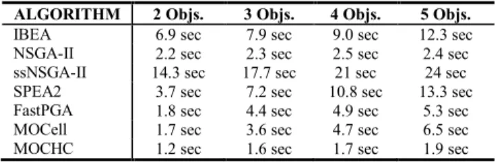
We show here representative run time figures, since there can be no precise run time measurement when it comes to any type of randomized algorithms. Table 7 shows run times for

all algorithms applied to the E-Shop feature model with 50,000 objective function evaluations.

TABLE 7:RUN TIME COMPARISON

ALGORITHM 2 Objs. 3 Objs. 4 Objs. 5 Objs.

IBEA 6.9 sec 7.9 sec 9.0 sec 12.3 sec

NSGA-II 2.2 sec 2.3 sec 2.5 sec 2.4 sec ssNSGA-II 14.3 sec 17.7 sec 21 sec 24 sec SPEA2 3.7 sec 7.2 sec 10.8 sec 13.3 sec FastPGA 1.8 sec 4.4 sec 4.9 sec 5.3 sec MOCell 1.7 sec 3.6 sec 4.7 sec 6.5 sec MOCHC 1.2 sec 1.6 sec 1.7 sec 1.9 sec

B. Quality Indicator Comparison

Table 8 shows our results. The algorithms are sorted on Hypervolume (HV) in the 5-objective, E-Shop measurements. In the 50-K runs, each algorithm run is repeated 10 times, each time making 50,000 evaluations of the objective functions. The median of the quality indicators (HV and spread) is reported. Also reported is the percentage of fully-correct solutions in the Pareto fronts, i.e. solutions that have zero violations, which is the first optimization objective. In the 50-M runs, each algorithms is run only once with 50 Million evaluations. Black cells with white font indicate results where IBEA performed much better than other algorithms, as discussed below.

All quality indicators in Table 8 are better when greater (see section III, subsection E). We do not have any reference measurements to compare to; therefore we only compare the different runs against one another.

Looking at the results in Table 8, we make the following observations:

 IBEA stands out in terms of HV, spread, and percentage of fully-correct solutions, as can be seen in the black cells with white font. The remarkable gains with this algorithm become obvious with the bigger, more complex E-Shop feature model, and with more objectives.

 We pay special attention to the better spread results that IBEA achieves, although IBEA does not incorporate crowd pruning measures in its dominance criteria. It outperforms the very algorithms that depend on crowd pruning.

 The remaining algorithms (NSGA-II, ssNSGA-II, SPEA2, FastPGA, MOCell, and MOCHC) perform moderately with the smaller Web Portal feature model with 2 and 3 objectives. With 4 or 5 objectives, or when applied to the bigger E-Shop feature model, these algorithms do not perform nearly acceptably when compared with the IBEA results. The least performing among these were MOCHC and SPEA2, especially with 4 and 5 objectives.

 In the 2-objective run for E-Shop, with 50 Million evaluations, all algorithms seem to yield the same results, with 100% of the Pareto front having zero violations, except for MOCHC, which fails miserably. After examining the resulting Pareto fronts, we find that IBEA outperforms in this category as well; since IBEA is able to find 3 solutions, each having zero violations and only one missing feature. Other algorithms only found one or two solutions, and some solutions had two missing features.

TABLE 8:COMPARISON OF QUALITY INDICATORS, SORTED ON HV IN 5-OBJ,E-SHOP 50M EVALS.

FM _RITHM ALGO

5 Objectives 4 Objectives 3 Objectives 2 Objectives

HV SPREAD CORRE% CT HV SPREAD % CORR ECT HV SPREAD % CORR ECT HV SPREAD % CORR ECT Web Portal (50K evals) IBEA 0.34 0.79 73% 0.43 1.18 56% 0.56 1.33 82% 1.00 1.04 14% NSGA-II 0.27 0.68 8% 0.39 0.74 8% 0.57 1.03 24% 1.00 1.04 14% MOCell 0.27 0.65 4% 0.38 0.68 8% 0.57 1.07 27% 1.00 0.95 20% ssNSGAII 0.27 0.70 6% 0.40 0.73 8% 0.57 1.15 31% 1.00 1.04 14% FastPGA 0.27 0.68 7% 0.40 0.71 9% 0.57 1.13 34% 1.00 1.04 14% SPEA2 0.27 0.54 0% 0.40 0.62 2% 0.57 0.86 13% 1.00 1.04 14% MOCHC 0.28 0.68 6% 0.42 0.65 7% 0.55 0.94 25% 1.00 0.95 20% E-Shop (50K evals) IBEA 0.21 0.77 0% 0.28 0.78 0% 0.40 1.01 0% 0.98 0.99 0% NSGA-II 0.17 0.72 0% 0.20 0.72 0% 0.34 0.71 0% 0.98 0.99 0% MOCell 0.16 0.70 0% 0.19 0.71 0% 0.32 0.70 0% 0.98 0.99 0% ssNSGAII 0.16 0.69 0% 0.20 0.68 0% 0.34 0.70 0% 0.98 0.99 0% FastPGA 0.16 0.67 0% 0.19 0.69 0% 0.33 0.71 0% 0.98 0.99 0% SPEA2 0.14 0.48 0% 0.19 0.55 0% 0.32 0.61 0% 0.98 0.99 0% MOCHC 0.14 0.66 0% 0.20 0.69 0% 0.31 0.72 0% 0.97 1.00 0% E-Shop (50M evals) IBEA 0.28 0.88 52% 0.37 1.15 42% 0.52 1.08 80% 1.00 1.00 100% NSGA-II 0.23 0.75 1% 0.25 0.81 1% 0.42 0.93 1% 1.00 1.00 100% MOCell 0.23 0.82 1% 0.25 0.86 1% 0.43 0.76 1% 1.00 1.00 100% ssNSGAII 0.22 0.73 1% 0.24 0.86 1% 0.41 0.87 1% 1.00 1.00 100% FastPGA 0.22 0.82 0% 0.25 0.81 1% 0.42 0.85 1% 1.00 1.00 100% SPEA2 0.20 0.55 0% 0.23 0.64 0% 0.39 0.60 0% 1.00 1.00 100% MOCHC 0.19 0.66 0% 0.23 0.70 0% 0.35 0.72 0% 0.97 0.99 0%

C. Further Runs with IBEA

In order to get a rough idea about how soon IBEA arrives at fully-correct solutions, we performed further runs on the E-Shop feature model with 5 objectives. The results are shown in Table 9.

The quickest results were 3 compliant configurations obtained within 8 minutes. Such results can be useful when a reasoned argument is needed quickly (e.g. at a meeting). Longer runs would be needed to get more optimized and better diversified results. While IBEA achieved 3 acceptable configuration in about 8 minutes, other algorithms took 50 million evaluations (about 3 hours) to find just one acceptable configuration.

TABLE 9:VARIOUS RUNS WITH IBEA ON E-SHOP,5 OBJECTIVES

Evals. Run Time HV Spread % Correct

50,000 12.3 sec 0.21 0.77 0% 1 Million 4 min 0.25 0.77 0% 2 Million 8 min 0.25 0.98 3% 5 Million 20 min 0.27 1.00 16% 10 Million 38 min 0.28 0.86 16% 20 Million 81 min 0.28 0.91 30% 50 Million ~ 3 hours 0.28 0.88 52%

D. Usefulness of the Pareto Fronts

We now closely study an example of the resulting Pareto Fronts to demonstrate their usefulness to product managers and software developers. These are the values that matter more to the end users than aggregate measures such as Hypervolume and Spread.

Table 10 shows portions of the Pareto front resulting from applying IBEA to the E-Shop feature model with five objectives. The values shown are those values to be minimized, as explained in section IV, subsection C. The rows are sorted on violations from smallest to largest.

TABLE 10:PORTIONS OF PARETO FRONT FOR IBEA ON E-SHOP,5OBJS. # Violations _Features Missing Not Used _Before Defects Cost

1 0 63 103 602 2204 2 0 65 101 604 2189 3 0 65 124 480 2122 4 0 67 123 471 2106 5 0 78 89 613 2033 … … … … 51 0 220 40 126 653 52 0 220 42 116 649 53 1 119 63 532 1587 54 1 123 62 509 1568 … … … … 64 2 231 28 147 554 65 2 235 26 135 516 66 3 209 31 242 750 67 3 211 31 227 724 … … … … 98 10 279 5 17 86 99 12 280 5 9 78

We first note that, out of 99 points on the Pareto front, 52 points had zero rule violations; 8 points had only 1 violation, 5 points had only 2 violations, and so forth. This result is especially remarkable compared to other algorithms. NSGA-II, ssNSGA-NSGA-II, and MOCell each resulted in only one point with zero violations. SPEA2, FastPGA and MOCHC did not result in any points with zero violations.

The major advantage of this set of feature configurations is that the product manager has 52 choices that are fully compliant with the feature model. Each one of these configurations is Pareto-optimal; i.e. no solution exists that can beat it in one objective while keeping the remaining objectives the same.

E. Fully-Correct vs. Marginally-Incorrect Results

Table 10 also shows quite a few solutions that are marginally-incorrect; i.e. solutions with a small number of violations. By nature of the Pareto front, and by examining these solutions against solutions with zero violations, one can assert that the other objectives (especially COST, DEFECTS) are either improved or at least not made worse. If the improvement in certain objectives is deemed significant, software developers can mitigate or work around the one or two rule violations in question, thus providing product managers with an even broader range of configuration choices.

VI. DISCUSSION

In this section, we reason about the findings of the experiment and their implications.

A. Indicator-Based Evolutionary Algorithm (IBEA) vs. Other MEOAs

We first tend to the question: why does IBEA perform so well? And why does it outperform commonly used algorithms? An explanation is provided in [27], where it is experimentally demonstrated with real-valued benchmark test functions that the performance of NSGA-II and SPEA2 rapidly deteriorates with increasing dimension, and that other algorithms like ε-MOEA, MSOPS, IBEA and SMS-EMOA cope very well with high-dimensional objective spaces. It was found that NSGA-II and SPEA2 tended to “increase the distance to the Pareto front in the first generations because the diversity-based selection criteria favor higher distances between solutions. Special emphasis is given to extremal solutions with values near zero in one or more objectives. These solutions remain non-dominated and the distance cannot be reduced thereafter.” All other algorithms used in this study (except IBEA) depend on evaluation criteria similar to NSGA-II or SPEA2, thus inheriting the same handicap at higher dimension; they tended to prune out solutions that crowded towards the much-desired zero-violation point, thus achieving low scores on the %correct measure.

IBEA, on the other hand, calculates a dominance value based on quality indicators that depend primarily on the user preferences. Thus IBEA has no need for a secondary evaluation criterion such as diversity of solutions. This

enabled IBEA to explore the various optimal solutions with zero-violations of model constraints.

This actually highlights IBEA’s ability to find correct as well as optimal solutions. Other algorithms focused on finding

optimal and diversified solutions, but failed in both, because they couldn’t explore the fully-correct solution space. Evolutionary search algorithms are not only meant for optimization, although they’re mostly used for that, but they’re also meant to find feasible solutions from a large space of possible combinations that may or may not conform to model constraints and dependencies.

B. Method for Achieving Product Correctness

In this experiment, we were able to generate many acceptable configurations with the help of evolutionary algorithms. Other researchers [12] included a repair operator to guarantee that each candidate solution conforms with the feature model before evaluating it for promotion to the next generation. They refrained from designing the objective function so that invalid solutions always score lower than valid solutions, because it was hard to do so with a single-objective fitness function. Having attempted the inclusion of correctness within another objective in order to guarantee correctness, we recognize this hardship. It was much easier for us to obtain correct solutions (especially with IBEA) by defining correctness as an objective of its own.

The results from this experiment show that our method is sufficient, but they do not preclude further research into other methods, including the possibility of designing new crossover and mutation operators which “know” the feature model and avoid tampering with its constraints while altering the decision string.

VII. THREATS TO VALIDITY

One issue with our analysis is the use of synthetic data as attributes of features, i.e. COST, DEFECTS, and

USED_BEFORE. The data were generated randomly based on distributions seen in historical data sets. The difficulty of obtaining real data comes from the fact that such numbers are usually associated with software components, not features. When available, such data is often proprietary and not published. Nevertheless, the results we obtained have such a large margin of superiority achieved by IBEA over other algorithms which couldn’t possibly be biased by the synthetic data. Future work should attempt to collect real data for use with IBEA and other MEOAs to best optimize product configuration.

Also, the various parameter settings of the MEOAs were fixed according to the default settings in jMetal. The focus was on comparing algorithms to one another while using the same parameter settings. A more thorough investigation might explore the effects of parameter fine-tuning.

A threat to external validity is that we are unable to generalize our findings to other software engineering problems. Nevertheless, we do provide a discussion of the problem characteristics that make IBEA perform best for the software product line domain, and we anticipate the same performance advantage when applying IBEA to problems with similar complexity and dimensionality.

VIII. CONCLUSIONS AND FUTURE WORK

The greatest conclusion of this experiment is the clear advantage IBEA search algorithm because of the way it exploits user preferences. This is the first time in software engineering research that IBEA is used, and it is shown to succeed and outperform often-used algorithms such as NSGA-II. In fact, we show that IBEA can arrive at acceptable configurations for the large E-Shop model with 5 objectives in as little as 8 minutes, while some absolute-dominance type algorithms found one acceptable configuration after 3 hours, and some couldn’t find any.

The solution diversity results, indicated by the spread values, were also superior for IBEA, although it is the one algorithm that does not include crowd pruning as a strategy. The reliance on crowd pruning by other algorithms not only caused stagnation afar from the true Pareto front, but also lesser diversity in the end result. This effect is worthy of further exploration both theoretically and experimentally.

The E-Shop problem was especially complex in the decision space, since a string of 290 decisions had to comply with 419 rules. Also, the objective space was 5-dimensional, which is rare in SBSE literature. Consequently, the results of this paper should propel the field into exploring the performance of IBEA compared to older results in various problems; attempting harder, more complex problems with this powerful tool; and holding more comparisons among available MEOAs applied to software engineering problems.

The other major finding is the ability to generate Pareto-optimal, feature-model-compliant configurations through an evolutionary algorithm (IBEA), by treating correctness as one of the optimization objectives and letting the optimizer “learn” its way into compliance. There was no need for a repair operator or special evolutionary operators that are custom-tailored to this domain. Still, the question may arise regarding the speed of convergence or the savings in computing power when this method is used as opposed to other methods, which may be the subject of future exploration.

Other directions for future work may be:

1- Examining scalability of the remarkable results obtained with IBEA with larger Feature Model, and possibly more optimization objectives.

2- Investigating the effects of parameter tuning with IBEA and other MEOAs.

3- Exploring minor differences among MEOAs reflected in the data collected here but not further investigated.

ACKNOWLEDGMENT

This research work was funded by the Qatar National Research Fund (QNRF) under the National Priorities Research Program (NPRP) Grant No.: 09-1205-2-470.

REFERENCES

[1] D. Benavides, A. Ruiz-Cortés, and P. Trinidad, "Automated Reasoning on Feature Models," in Proc. CAISE, 2005, pp. 491-503.

[2] D. Benavides, S. Segura, and A. Ruiz-Cortes, "Automated analysis of feature models 20 years later: A literature review,"

Information Systems, vol. 35, no. 6, pp. 615-636, 2010.

[3] T. Berger, S. She, R. Lotufo, A. Wasowski, and K. Czarnecki, "Variability Modeling in the Real: A Perspective from the Operating Systems Domain," in Proc. ASE, Antwerp, Belgium, 2010, pp. 73-82.

[4] M. Bowman, L.C. Briand, and Y. Labiche, "Solving the class responsibility assignment problem in object-oriented analysis with multi-objective genetic algorithms," IEEE Transactions on Software Engineering, vol. 36, no. 6, pp. 817-837, 2010. [5] T. E. Colanzi, W. Assuncao, S. R. Vergilio, and A. Pozo,

"Generating Integration Test Orders for Aspect-Oriented Software with Multi-objective Algorithms," in Latin American Workshop on Aspect-Oriented Software Development, 2011. [6] J. Coplien, D. Hoffman, and D. Weiss, "Commonality and

Variability in Software Engineering," IEEE Software, vol. 15, no. 6, pp. 37-45, 1998.

[7] K. Deb, A. Pratap, S. Agarwal, and T. Meyarivan, "A fast and elitist multiobjective genetic algorithm: NSGA-II," IEEE Transactions on Evolutionary Computation, vol. 6, no. 2, pp. 182-197, 2002.

[8] J. J. Durillo and A. J. Nebro, "jMetal: A Java framework for multi-objective optimization," Advances in Engineering Software, vol. 42, pp. 760-771, 2011.

[9] J.J. Durillo, A.J. Nebro, F. Luna, and E. Alba, "On the effect of the steady-state selection scheme in multi-objective genetic algorithms," in 5th International Conference on Evolutionary MultiCriterion Optimization, 2009, pp. 183-197.

[10] H. Eskandari, C. D. Geiger, and G. B. Lamont, "FastPGA: A dynamic population sizing approach for solving expensive multiobjective optimization problems," in Proceedings of EMO, 2007, pp. 141-155.

[11] S. Gueorguiev, M. Harman, and G. Antoniol, "Software Project Planning for Robustness and Completion Time in the Presence of Uncertainty using Multi Objective Search Based Software Engineering," in Proc. GECCO, 2009, pp. 1673-1680.

[12] J. Guo, J. White, G. Wang, J. Li, and Y. Wang, "A genetic algorithm for optimized feature selection with resource constraints in software product lines," Journal of Systems and Software, vol. 84, no. 12, pp. 2208–2221, December 2011. [13] M. Harman, "The Current State and Future of Search Based

Software Engineering," in Proc. FOSE, 2007, pp. 342-357. [14] M. Harman and B. F. Jones, "Search based software

engineering," Information and Software Technology, vol. 43, no. 14, pp. 833–839, December 2001.

[15] M. Harman, K. Lakhotia, and P. McMinn, "A Multi-Objective Approach to Search-based Test Data Generation," in Proc. of GECCO, London, UK, 2007, pp. 1098–1105.

[16] M. Harman, S. A. Mansouri, and Y. Zhang, "Search Based Software Engineering: A Comprehensive Analysis and Review of Trends Techniques and Applications," King’s College, London, UK, Technical Report TR-09-03, 2009.

[17] W. Heaven and E. Letier, "Simulating and Optimising Design Decisions in Quantitative Goal Models," in Proc. RE, 2011, pp. 79-88.

[18] K. Kang, J. Lee, and P. Donohoe, "Feature-Oriented Product Line Engineering," IEEE Software, vol. 19, no. 4, pp. 58-65, Jul/Aug 2002.

[19] S. Q. Lau, "Domain analysis of e-commerce systems using feature-based model templates," Dept. Electrical and Computer Engineering, University of Waterloo, Canada, Master's Thesis 2006.

[20] M. Mendonca, T. Bartolomei, and D. Cowan, "Decision-making coordination in collaborative product configuration," in ACM Symposium on Applied Computing, 2008.

[21] M. Mendonca, M. Branco, and D. Cowan, "S.P.L.O.T. - Software Product Lines Online Tools," in Proc. OOPSLA, Orlando, USA, 2009.

[22] A.J. Nebro et al., "Optimal antenna placement using a new multi-objective CHC algorithm," in Proceedings of the 9th annual conference on Genetic and evolutionary computation, New York, NY, USA, 2007, pp. 876-883.

[23] A.J. Nebro, J.J. Durillo, F. Luna, B. Dorronsoro, and E. Alba, "Mocell: A cellular genetic algorithm for multiobjective optimization," Int. J. Intelligent Systems, vol. 24, no. 7, pp. 726-746, 2009.

[24] K. Pohl, G. Böckle, and F. J. van der Linden, Software Product Line Engineering. New York: Springer-Verlag, 2005.

[25] A. S. Sayyad and H. Ammar, "Pareto-Optimal Search-Based Software Engineering: A Literature Survey," in Proc. RAISE, San Francisco, USA, 2013.

[26] A. S. Sayyad, H. Ammar, and T. Menzies, "Feature Model Recommendations using Data Mining," in Proc. RSSE, Zurich, Switzerland, 2012.

[27] T. Wagner, N. Beume, and B. Naujoks, "Pareto-, Aggregation-, and Indicator-Based Methods in Many-Objective Optimization," in Proc. EMO, LNCS Volume 4403/2007, 2007, pp. 742-756. [28] J. White, B. Dougherty, and D. C. Schmidt, "Selecting highly

optimal architectural feature sets with Filtered Cartesian Flattening," Journal of Systems and Software, vol. 82, no. 8, pp. 1268–1284, August 2009.

[29] J. White, B. Dougherty, D. C. Schmidt, and D. Benavides, "Automated reasoning for multi-step feature model configuration problems," in Proc. SPLC, San Francisco, USA, 2009, pp. 11-20.

[30] S. Yoo and M. Harman, "Pareto efficient multi-objective test case selection," in Proc. ISSTA, 2007, pp. 140-150.

[31] Y. Zhang, M. Harman, and S. A. Mansouri, "The Multi-Objective Next Release Problem," in Proc. GECCO, 2007, pp. 1129-1136.

[32] G. Zhang, H. Ye, and Y. Lin, "Using Knowledge-Based Systems to Manage Quality Attributes in Software Product Lines," in

Proc. SPLC, 2011.

[33] E. Zitzler and S. Kunzli, "Indicator-based selection in multiobjective search," in Parallel Problem Solving from Nature. Berlin, Germany: Springer-Verlag, 2004, pp. 832–842. [34] E. Zitzler and Thiele L., "Multiobjective evolutionary

algorithms: a comparative case study and the strength pareto approach," IEEE Transactions on Evolutionary Computation, vol. 3, no. 4, pp. 257–271, 1999.

[35] E. Zitzler, M. Laumanns, and L. Thiele, "SPEA2: Improving the strength pareto evolutionary algorithm," in Evolutionary Methods for Design, Optimization and Control with Applications to Industrial Problems. Athens, Greece, 2001, pp. 95-100.