Volume Title: NBER Macroeconomics Annual 2008, Volume 23
Volume Author/Editor: Daron Acemoglu, Kenneth Rogoff and Michael
Woodford, editors
Volume Publisher: University of Chicago Press
Volume ISBN: 0-226-00204-7
Volume URL: http://www.nber.org/books/acem08-1
Conference Date: April 4-5, 2008
Publication Date: April 2009
Chapter Title: The Timing of Labor Market Expansions: New Facts and a New
Hypothesis
Chapter Author: Giuseppe Moscarini, Fabien Postel-Vinay
Chapter URL: http://www.nber.org/chapters/c7270
The Timing of Labor Market Expansions:
New Facts and a New Hypothesis
Giuseppe Moscarini,Yale University and NBER
Fabien Postel‐Vinay,University of Bristol and Université de Paris I (Panthéon‐Sorbonne)
I. Introduction
The cyclical behavior of (un)employment and wages still poses a for-midable challenge to macroeconomists. No other aspect of the business cycle has been as widely studied and remains as poorly understood. While a consensus has slowly emerged on the importance of search fric-tions to explain equilibrium unemployment, as well as residual wage inequality unexplained by observable worker and firm characteristics, we still do not know how wages are set in practice. When labor de-mand rises, driven by higher productivity or real dede-mand for goods, how is it exactly that workers obtain higher wages? And why do wages rise gradually and slowly over business cycle expansions?
The search‐and‐matching business cycle literature commonly as-sumes that wages are settled through a bargaining process but does not identify the source of parties’bargaining power. The search litera-ture on wage inequality, invariably cast in steady state and abstracting from aggregate fluctuations, typically assumes that firms have full monopsony power and make take‐it‐or‐leave‐it offers of employment contracts. To reconcile this intuitive and plausible assumption with the reality of worker rents and wage inequality and to avoid the Diamond (1971) paradox, Burdett and Mortensen (1998) identify the source of workers’bargaining power in a form of moral hazard. Specifically, work-ers obtain more than their reservation wage in order to be induced to quit their previous employer and, once hired, to decline future outside offers. Poaching is the engine of wage growth and differentiation for individual workers.
In this article we argue that the same poaching mechanism also trans-mits aggregate productivity shocks to wages and employment. Firms offer higher wages only when they run out of cheap unemployed job
© 2009 by the National Bureau of Economic Research. All rights reserved. 978‐0‐226‐00204‐0/2009/2008‐0101$10.00
applicants and find it profitable to steal employees from their competi-tors, who in turn fight back and start paying more to retain their work-ers. Our argument builds on a set of new facts about aggregate dynamics in U.S. labor markets over the last two decades that we docu-ment by drawing in part from newly available data sets. These facts suggest a new view of how business cycles evolve and mature. We in-vestigate whether this view is consistent with the transitional dynamics of the Burdett‐Mortensen equilibrium search model. In Moscarini and Postel‐Vinay (2008), we develop the first theoretical analysis of the out‐ of‐steady‐state behavior of the Burdett‐Mortensen model.1In the present paper, we build on those results and present a quantitative simulation exercise to gauge the extent to which the Burdett‐Mortensen model’s quantitative predictions are congruent with the facts that we uncover. The three new facts concern three seemingly unrelated time series. First, the share of employment at small firms and establishments de-clines through the 1990s and 2000s expansions and crosses below its overall average around the middle of each decade; in contrast, large firms are hit particularly hard by recessions and then slowly recover employment share. Alternatively, the difference between the growth rate of employment at large firms/establishments vis‐à‐vis small ones is strongly procyclical, its troughs and peaks roughly coinciding with NBER business cycle dates and rising uniformly in between. Second, the monthly employer‐to‐employer (EE) worker transition rate declines through the first half of each decade and rebounds starting in 1996 and in 2004. Large employers poach more than small ones late in the 1990s, not so after the ensuing recession. Third, various measures of detrended worker compensation exhibit a behavior quite similar to the EE rate, both economywide and for each employer size class, with workers at larger employers earning more at all points in time. All in all, simulta-neously and at the midpoint of the expansion, several years after the previous trough, the unemployment rate crosses below trend, large em-ployers take over net job creation, workers start quitting more from job to job, and wages accelerate.
These facts suggest the following view of aggregate expansions. Fol-lowing a positive aggregate shock to labor demand, wages respond lit-tle on impact and start rising when firms run out of cheap unemployed hires and start competing to poach and to retain employed workers. Early in an expansion, the large pool of unemployed workers sustains firms’ monopsony power. Wages remain low, firms hire mostly from unemployment, and relatively few workers quit from job to job. As the reservoir of unemployment dries out, more productive firms find
it profitable to start raising wages to raid workers from less productive competitors. They respond by paying their workers more to retain them. Wages rise both within firms and as workers upgrade by quit-ting to higher‐paying employers. Workers quit mostly from small, low‐ paying firms to large, high‐paying firms. The growth in the employment of large firms is fueled by the stock of employment at small firms, which takes some time to replenish after a recession. Hence, employment at small firms grows faster and peaks earlier than at large firms. As em-ployment at small firms peaks and poaching becomes a more important source of hiring, the EE rate picks up.
The facts that we highlight and use to support the above view of la-bor market expansions are limited in time and scope by data availabil-ity. The bulk of our data cover only the last two expansions, which have been uniquely“jobless.”Thus we do not claim to have identified new business cycle stylized facts. What we do claim is that the patterns we point out for the last two expansions shed some light on the workings of labor markets in general, mainly by identifying the hiring behavior of large firms as an important channel for the propagation of aggregate shocks.
We formalize those views within a wage‐posting model à la Burdett and Mortensen. A calibrated example of the transitional dynamics of the wage‐posting model, following an aggregate productivity shock, exhibits many of the qualitative features of our new facts. Larger firms pay more at any point in time. Employment growth is faster at small firms early on, and then large firms take over as they poach employees. Wages rise slowly at first and then accelerate. The job‐to‐job quit rate rises for some time as the pool of workers at small firms, vulnerable to poaching, expands.
A detailed theoretical analysis of the transitional dynamics of the Burdett‐Mortensen model, which we simulate in this paper, is available in Moscarini and Postel‐Vinay (2008). Because of the known complexity of this problem, in the present paper we restrict attention to a certain class of equilibria (which we callrank‐preserving), as defined and moti-vated in the text. We further confine the analysis to the deterministic transition to a steady state following an unanticipated, permanent ag-gregate productivity shock. Before the shock, firms pay constant wages in a stationary world. After the shock, firms post and commit to new contracts that pay wages contingent only on either calendar time or the unemployment rate. All workers in a firm are paid the same wage, no matter when hired or from where. Workers receive offers both off and on the job and decide which ones to accept on the basis of their
implied present discounted value of wages, taking future transitions into account.
In our computed example, firms back‐load wages to the late part of the expansion. In steady‐state analysis of wage‐tenure contracts, wages are back‐loaded late in the employment relationship to piggyback on future poachers. If workers are risk neutral, back‐loading is extreme in the form of a step function of tenure (Stevens 2004). Gradual wage growth requires risk aversion and extreme market incompleteness as a motive for consumption smoothing (Burdett and Coles 2003). In our setup, wages grow slowly even if workers are risk neutral and capital markets are perfect; wage back‐loading occurs over calendar time, not over tenure. Beyond the piggybacking motive, the increasing scarcity of cheap hires from unemployment makes raising wages more attractive in order to poach employed workers, thus also to retain own employees.
While the process of upgrading from job to job is usually described as climbing a wage ladder, our non‐steady‐state analysis reveals that it is best described as jumping from a“wage escalator”up to a higher one. All workers benefit as wages rise within firms. In addition, job changers rise from one rising wage profile to a higher one at another firm. There-fore, aggregate wages rise for two reasons: on the intensive margin, all workers are paid progressively more, and on the extensive margin, workers move to higher‐paying firms.
In our example, job changers exhibit faster (so, in this limited sense, more procyclical) wage growth than job stayers. This prediction is con-sistent with the main findings of the literature on real wage cyclicality (Bils 1985; Beaudry and DiNardo 1991; Solon, Barsky, and Parker 1994). This literature, however, has been hampered by the lack of high‐frequency, reliable information on job‐to‐job transitions in a repre-sentative sample. We present such evidence from the monthly Current Population Survey (CPS) starting in 1994, when it first became avail-able, but we have not yet linked it to individual wage information. A similar view holds that workers flow from low‐wage to high‐wage in-dustries in an expansion, a“cyclical upgrading of labor”(Okun 1973). This is based on the observation that high‐wage industries have more cyclical employment. Barlevy (2001), however, shows that the inter-industry wage gains reflect to some extent the compensating differential associated with accepting riskier jobs. While the source of interindustry wage differentials is still an open question, we show that the patterns of employment growth by firm and establishment size that we uncover hold within, and not across, industries.
Our example also features a strong propagation in wages and labor productivity, which keep rising years after the initial shocks, although the unemployment rate transition’s half‐life is just a few months. The main reason is that job‐to‐job transitions in the data are an order of magnitude slower than the reallocation from unemployment to em-ployment. Thus, the upgrading process is slow, and so is the rise in labor productivity after an initial jump following the shock. The propagation is less pronounced for the EE rate. We are, however, ignoring further sources of propagation of the unemployment rate, such as endogenous labor force participation. This is likely to rise in the expansion, feeding the market with relatively cheap candidates for hiring from unemploy-ment and delaying the mounemploy-ment when large firms have to start raising wages aggressively to poach workers, the small firms have to respond to retain them, and the EE rate peaks.
Section II lays out the facts and offers an intuitive explanation of them based on the Burdett‐Mortensen equilibrium search model. The rest of the paper discusses the theoretical model and its quantitative predictions. Section III describes the basic economic environment. Sec-tion IV characterizes the dynamic labor market equilibrium and explains our solution strategy. Details and results of a simple calibration exercise are presented and discussed in Section V. Finally, Section VI presents conclusions and gives some thoughts about possible further research avenues.
II. Aggregate Labor Market Fluctuations: New Evidence
A. Definitions and Overview
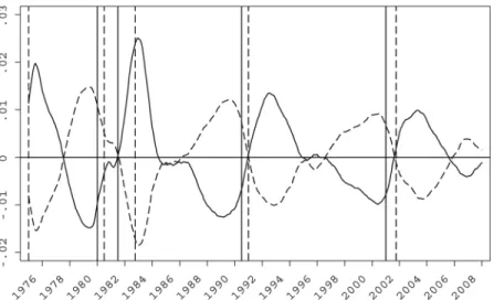
In order to organize the new evidence under a common heading, we open this section by providing our own definition of a tight labor mar-ket. We apply an HP (Hodrick‐Prescott) filter to both the monthly ci-vilian unemployment rate and the monthly cici-vilian employment to working‐age population ratio (E/POP ratio) from the Bureau of Labor Statistics (BLS) in 1948:1–2008:1. We choose a smoothing parameter equal to 10532:25, which corresponds to Shimer’s (2005) choice of 105at a quarterly frequency.2In figure 1 we plot the deviations of the unemployment rate and the E/POP ratio from their respective postwar trends.3 We show the resulting detrended series by zooming only on 1975–2008, because this is the longest span covered by our other data series. Clearly, the unemployment rate crosses its trend from above in 1977, 1984–85, 1995–96, and 2005. In the second and third episodes, it
hovers around trend for almost 2 years but is higher before and lower after that point in time during an expansion, further corroborating our detrending choice.
Armed with this graph, we define the labor market to betightwhen the unemployment rate first falls below its trend and remains there for at least a year thereafter. The window of at least 12 months of consecu-tive observations above or below trend, before/after first crossing it, is necessary to eliminate neutral phases, when the unemployment rate hovers near trend. Notice that this definition does not coincide with that of an expansion or recession according to NBER dates (materi-alized on all figures by vertical lines, solid for peaks and dashed for troughs). Indeed, the phases of labor market neutrality occur typically roughly midway between troughs and peaks, although the unemploy-ment rate itself does not have symmetric dynamics, typically rising faster than it declines. From every cyclical trough in the sample period, the la-bor market starts slack, then shifts into neutral, and finally tightens, until the next peak.
Although we have chosen to couch this definition in terms of the un-employment rate, it is evident from figure 1 that the E/POP ratio is an equally good indicator of labor market tightness as defined above, since
Fig. 1. Employment and unemployment rates. The solid line is the unemployment rate. The dashed line is the E/POP ratio. HP‐filtered U.S. monthly data, 1978:1–2008:1. HP trends are calculated over the entire postwar series (1948:1–2008:1) with smoothing parameter 10532:25, then MA smoothed. The solid (dashed) vertical line indicates
the cyclical behavior of the E/POP ratio is essentially the mirror image of that of the unemployment rate (the correlation coefficient of the two series over the entire postwar period is−0.92). In other words, as far as labor market cycle dating is concerned, cyclical variations in labor force participation can be ignored to a first approximation. We will implicitly make this approximation throughout the paper, especially in the theory in which the participation margin will be shut down altogether.
The three new facts that we uncover and document in this section concern three seemingly unrelated time series in the last few decades. Armed with our definition of tight and slack labor markets, we can briefly characterize them as follows. We first describe them verbally and later graphically rather than reporting correlations of detrended se-ries, because many of the available time series cover only a couple of busi-ness cycles.
Fact 1. Small firms and establishments grow in size faster than large ones when the labor market is slack, and vice versa when the labor market turns tight. Therefore, the firm/establishment size distribution gets com-pressed in a slack labor market and becomes more unequal in a tight one. Fact 2. The rate at which employed workers quit to other jobs is above trend in a tight labor market and below trend in a slack labor market.
Fact 3. The annual growth rate of real wages or weekly earnings is above its trend in a tight labor market and below in a slack labor market.
We now describe the three facts in detail.
B. The Cyclical Dynamics of the Firm/Establishment Size Distribution Most of the new empirical evidence that we present in this paper per-tains to fact 1, the relative timing of net job creation within a business cycle by size classes. Essentially, of the total job creation observed from cyclical trough to peak, more of it occurs early on in the expansion for small firms/establishments than for larger ones. In recessions, large firms/establishments are hit particularly hard. Notice that this fact does not say that most job creation occurs at small establishments, a well‐ known subject of political rhetoric and confusion. Our finding is about the movement of the relative growth rate. While the political debate is typically focused on growth rates, it is still the case that the number of jobs added by large establishments is higher than that added by small ones or by entrants at nearly all points in the aggregate expansion.4
Reflecting the dual structure of its statistical agencies, the U.S. federal government has produced two comprehensive and independent
sources of information on firms and establishments, specifically on their count, employment, payroll, industry, and location. Business Employ-ment Dynamics (BED) is a data set providing quarterly information on job flows and firm sizes since 1992. It is based on the quarterly Census of Employment and Wages, which in turn collects information from the state and federal Unemployment Insurance (UI) systems accruing to the BLS for this purpose. The BED covers all employers subject to UI taxes, which account for 98% of employment. While used primarily to mea-sure job flows, information on employment stocks is publicly available when aggregated into nine classes of firm size.5
The second data set is the County Business Patterns (CBP), which is maintained at the Bureau of the Census and derives from the Business Register and quinquennial economic censuses. The publicly available information from the CBP that we have been able to secure consists of annual information on counts, employment, industry, payroll, and location for all U.S. firms (since 1988) and establishments (since 1990), as well on nonemployers (self‐employed) for 1992 and 1997–2005. Lim-ited longitudinal information on employment growth by initial firm size in CBP is publicly available, under the name of Business Informa-tion Tracking Series (BITS) at the Census Bureau and Dynamic Size In-formation at the Small Business Administration.6
1. Employment Shares and Growth Rates by Size Classes
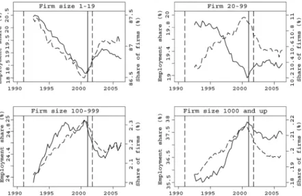
The firm size distribution series from BED, available in 1992–2007, show that small (in terms of employment) firms had a countercyclical share of total employment. They concentrated most of their job creation in the early part of the 1990s expansion and promptly expanded their employ-ment after 2001. Conversely, large firms concentrated most of their 1990s job creation after 1996 and again failed to create jobs in the first part of the 2000s expansion. This pattern is observed across nine firm size classes and is exemplified in figure 2, which plots employment shares for four different classes. The recoveries of the early 1990s and 2000s were
“jobless”mainly at large firms, whereas the strong job creation of the late 1990s, in the mature phase of the expansion, was concentrated mainly in large firms.7
The evidence for firms from BED can also be illustrated in terms of growth rates of employment rather than employment shares. The top two panels of figure 3 plot average employment growth rates of large and small firms. The bottom two panels report the difference in average employment growth rates between large and small firms (the two series
line indicates NBER peaks (troughs). Source: BED (quarterly) and authors’calculations.
Fig. 3. Difference in average growth rates of employment across firm size classes. Differential firm size growth, MA smoothed. The solid (dashed) vertical line indicates NBER peaks (troughs). Source: BED and authors’calculations.
on the corresponding top panel): when the series is positive, large firms grow faster, and vice versa.8The two columns of figure 3 relate to two different definitions of the“small”and“large”classes, as indicated on each panel. This highlights more vividly the pattern of figure 2: wher-ever one places the cutoff between small and large firms, small firms appear to have grown (relatively) faster than large firms at the begin-ning of the 1990s expansion and slower later on in that same expansion. A similar pattern seems to appear again at the beginning of the 2000s expansion. Focusing on the top two panels of figure 3, one can further decompose that pattern by noticing that average size growth of small firms actually trends down over the expansion, whereas that of large firms does not trend. This is why large firms take over on average. Hence these series of average growth rates by firm size class, albeit all clearly procyclical, diverge to some extent.
To further illustrate this pattern, figure 4 shows the comovements be-tween growth differentials across firm size classes (the series on the right panel of fig. 3) and the aggregate unemployment rate.9Although the two series fluctuate with a different amplitude, one sees that they exhibit very strong comovements: the correlation between growth rate differentials and the unemployment rate series is about−0.76 over the observation window.10
Fig. 4. Growth rate differentials, employment, and unemployment rates. The solid line is differential firm size growth, and the dashed line is the unemployment rate. All series are MA smoothed. The solid (dashed) vertical line indicates NBER peaks (troughs). Source: BED, BLS, and authors’calculations.
Similar firm‐level evidence can be constructed at an annual fre-quency, but beginning in 1988, from the CBP data, which are available at the firm (as well as establishment) level. CBP conveys only informa-tion on employment shares, which is our main focus, and not on firm counts, since this particular version of the data aggregates nonemployers with small firms in some years and not in others. This inconsistency makes cross‐date comparisons of firm counts impossible but does not affect employment since we have been excluding the self‐employed throughout. Figure 5 repeats figures 2 and 3 using CBP firm‐level data and confirms the pattern already observed in BED, not only for the 1990s and early 2000s but also around the previous recession, since we now also encompass 1988–91.
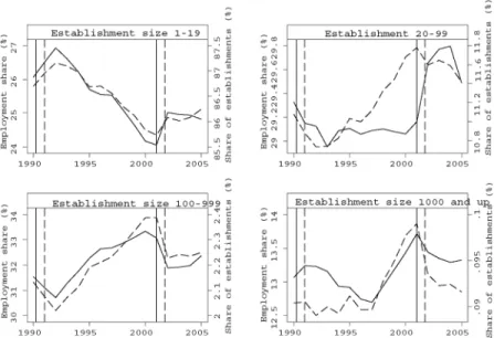
While the distinction between firms and establishments is often a thorny issue in theoretical exercises, fortunately for us this will not be the case. The same empirical phenomenon emerges from establishment‐ level data using the CBP since 1990 (see fig. 6, which replicates fig. 2 for establishments). The pattern of establishment size dynamics over the last two business cycles closely resembles that of firm size dynamics, partly owing to the fact that most (small) firms are mono‐establishment. More generally, however, large establishments tend to be part of large
Fig. 5. Employment shares and employment growth by firm size classes, CBP firm‐level data. Employment shares (top row) and growth rates (bottom row). The solid (dashed) vertical line indicates NBER peaks (troughs). Source: CBP (firm‐level data set) and authors’ calculations.
firms. If one looks across firm size bins in the CBP, the correlation be-tween the average number of establishments of the firm and the aver-age size of employment per establishment is close to one.
Overall, we conclude that large firms and establishments grow rela-tively faster when the labor market is tight according to our earlier definition, and vice versa for small ones.
2. The Reclassification Bias
While our last statement might appear plausible and intuitive, the following issue still needs to be resolved: the identity of firms in different size classes changes over time. Firms and establishments are reclassified at each obser-vation date according to their new size. Indeed the BED data set explicitly applies“dynamic allocation”of firms to size classes; that is, it even changes class assignments at an infraquarterly frequency for firms cross-ing the line between two size classes. Thus, in a growcross-ing economy, where firms gain size on average, one would expect the distribution of firm size to rise in a stochastic dominance sense. We refer to this issue as the reclas-sification bias.
To eliminate reclassification, we need longitudinal links on firms/ establishments to fix their assignment to size classes (or average wage
Fig. 6. Employment shares by establishment size. The solid (dashed) vertical line indicates NBER peaks (troughs). Source: CBP (yearly) and authors’calculations.
classes, or value‐added classes) at a cyclical trough then track over the expansion the shares of employment at these classes of employers, without reclassifying them every period. This would allow us to verify, for example, whether firms/establishments that are initially small often leapfrog and overtake the initially larger ones, a phenomenon that would invalidate our interpretation of the facts.
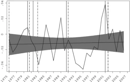
To this purpose, we utilize two publicly available longitudinal data sets on U.S. firms. The first is Compustat, which comprises only listed companies. We fix firm identities in 1975 and classify them once and for all in size bins (by employment): large above 5,000 employees and small fewer than 5,000. The reason for the large size cutoff is that listed companies are very large. Then, for each year from 1976 to 2005, we calculate the growth rate of employment over the past year at (initially) large firms and subtract the growth rate of the other initially small firms in the sample. We plot this difference in growth rates in figure 7 in a way that mimics figure 3. Consistent with the pattern uncovered in the BED, over three full business cycles this difference in growth rates is procyclical and crosses zero when the labor market turns tight.
Compustat is not a representative sample, but the CBP is. Although the underlying source of micro data is not publicly available, the Cen-sus Bureau publishes employment growth by firm size, where firms are
Fig. 7. Growth rate differentials across size classes for a fixed sample of publicly traded U.S. companies classified by size in 1975. Differential firm size growth: over 5,000 minus under 5,000 employees. The solid (dashed) vertical line indicates NBER peaks (troughs). Source: Compustat North American files and authors’calculations.
assigned to categories according to size on March 12 each year and stay in the same class for 1 year.11This data set, BITS, exploits the longitudi-nal links in CBP for just one year at a time. In figure 8 we plot our find-ings from BITS, again in terms of differences in growth rates. Every year since 1989, that is, since BITS data are publicly available, we com-pute the growth rate of employment over the subsequent year among firms that started above 500 employees in March of yeartand subtract the growth rate for the 1–499 employees size class. A positive number indicates that firms that were larger in March of yeartgrew faster than the other ones until March of yeartþ1, when they were reclassified after the relevant growth rates were computed. The evidence is again fairly clear‐cut, whether one detrends or not: small firms grow faster early in an expansion; the pattern then slowly reverses, to switch back abruptly during recessions. The differences in annual size growth rates are large.
3. Industry‐Level Evidence
An additional appeal of the CBP/BITS data set is that it provides industry‐ level information. This enables us to gauge whether the pattern identified in this subsection is also observed within industries or whether it mostly reflects a reallocation of labor across industries. More specifically, is it the
Fig. 8. Growth rate differentials across size classes for all U.S. firms, reclassified every year in March after computing the growth rate over the past year. Differential firm size growth: over 500 minus under 500 employees. The solid (dashed) vertical line indicates NBER peaks (troughs). Source: BITS and authors’calculations.
case that small firms exhibit faster growth at early stages of an expansion whereas large firms take over later on uniformly across industries, or is it that job creation early on is concentrated at industries that tend to be populated by smaller firms, whereas industries with larger firms have a
“slower start”? The answer turns out to be the former.
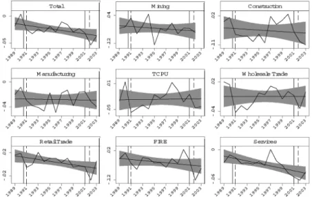
Figure 9 plots series equivalent to the one displayed in figure 8 for eight broad industries.12 Although industry‐level data are inevitably more noisy, the aggregate pattern shown on the upper‐left panel (a rep-etition of fig. 8) seems by and large to apply across industries. In all cases, without exceptions, the disaggregated industry series drop on or around recessions. Those series cross the trend from below only around 1996 in five of the eight industries: construction; transportation, communication, and public utilities (TCPU); wholesale trade; finance, insurance, and real estate (FIRE); and services. The pattern is similar in manufacturing, except for the sharp drop in 1996. Manufacturing is the industry in which the firm/employment size distribution is most skewed toward large values, an outlier in the economy at large, so small firms play a lesser role. In fact, the largest size cutoff available in BITS is 500 employees, which is well above the median firm size for all industries but is well below the median for manufacturing; so this data set is not really informative for manufacturing, where the vast
Fig. 9. Growth rate differentials across size classes for all U.S. firms, size classes fixed over a year, by industry. Differential firm size growth: over 500 minus under 500 employees. The solid (dashed) vertical line indicates NBER peaks (troughs). Source: BITS and authors’calculations.
majority of firms need to be classified as“large.”13The pattern is less clean in retail trade, but even there small firms grow faster early on after the recessions. Mining is the only (small) industry that does not fit the general picture at all. The effect on the other ( between‐industry) margin can also be assessed using the BITS data, for instance, by look-ing at the difference in employment growth between industries popu-lated by firms whose size is above the economywide average and industries with comparatively smaller firms. A plot of this difference (not reported here) suggests that this between‐industry difference has no particular cyclical pattern, contrary to the within‐industry series plotted in figure 9. This finding will make an interesting contribution to our discussion of how to interpret the facts below.
C. The Cyclical Dynamics of Employer‐to‐Employer Transitions
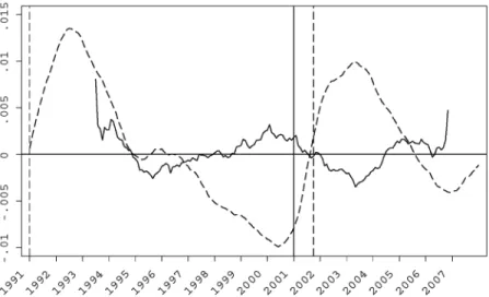
Monthly CPS data available since 1994 allow the construction of monthly EE transition rate series.14Such a series, compiled by Moscarini and Thomsson (2007), is plotted in figure 10 (in deviation from HP trend), to-gether with the unemployment rate series from figure 1 to highlight the EE rate’s cyclical behavior in terms of our adopted definition of labor market tightness.
Fig. 10. Monthly transition rate of employed workers to other employers. The solid line is the EE rate, and the dashed line is the unemployment rate. EE rate: U.S. monthly data, deviation from linear trend, MA smoothed. The solid (dashed) vertical line indicates NBER peaks (troughs). Source: CPS, BLS, Moscarini and Thomsson (2007), and authors’ calculations.
Our guiding hypothesis relates the time and cross‐employer varia-tion in poaching activity to wage growth. Publicly available data from the Census’s Survey of Income and Program Participation (SIPP)15 con-veys information about the workforce size of an individual’s current employer (employing establishment) as well as individual job histories. This allows a crude analysis of the poaching activity of establishments as a function of their size. Figure 11 plots a measure of the fraction of new hires coming from another employer (i.e., following an EE transi-tion) for three categories of hiring establishment size.16In other words, it plots a measure of the importance of poaching in the recruitment ac-tivity of establishments, by size of the hiring establishment. Changes in the design of the SIPP and other data limitations restrict the period over which that indicator can be constructed to the years shown on figure 11. While this admittedly constitutes very limited evidence, we still notice the following two points. First, and consistent with the evidence pre-sented in figure 10, poaching was more intense in the latter half of the 1990s expansion than in the immediate aftermath of the 2001 recession. This is true for all three categories of establishment size. Second, larger establishments almost always poach more than smaller ones. This differ-ence in“poaching intensity,”however, is more pronounced in 1997–99, when the labor market turns tight, than in 2002–4, when it is slack.
Fig. 11. Poaching and establishment size. The fraction of new hires coming from other employers, by establishment size category. The solid (dashed) vertical line indicates NBER peaks (troughs). Source: SIPP and authors’calculations.
D. The Cyclical Dynamics of Wages and Earnings
Third, and finally, we revisit the age‐old issue of real wage cyclicality. Our hypothesis is that the evolution of employment by firm size and job‐to‐job transitions fuel aggregate wage growth. Publicly available data from the BLS Current Employment Statistics on average monthly real (weekly and hourly) earnings show, after standard HP detrending, a behavior similar to that of the other variables that we have studied so far: flat in the first part of an expansion and sharply increasing later on. This occurs in every complete U.S. business cycle in 1964–2006, with the only exception of the 1980s, when a sharp decline in real wages of un-skilled workers gave rise to the well‐known increase in wage inequality. We do not report these raw data, but in order to isolate the pure cyclical effect, we first attempt to control for composition effects in employment over a suitably long time period.
We gather information on earnings, hours, and demographics from the Merged Outgoing Rotations of the monthly CPS, starting in 1982 when they became available. We take percentage wage growth over subsequent 12 months for the same individual as the object to be ex-plained in order to eliminate fixed effects in wage levels. Results for weekly earnings rather than hourly wages are very similar. We regress wage growth on many demographics to capture also composition ef-fects by observables in wage changes. Since we have only two observa-tions on wage levels and one on wage growth per individual, we cannot estimate individual fixed effects in growth rates. Finally, we plot the median residual from this regression month by month in figure 12. We also plot the 52nd percentile of the residual distribution in order to take into account the proportion of top‐coded earnings (between 0% and 2% per month), which create a spurious mass of zero or very low wage growth. The unemployment rate (again in deviation from HP trend) is also superimposed to gauge cyclicality. Relative to the first month, January 1982, rescaled to zero, unexplained wage growth is pos-itive in the late 1980s and especially late 1990s, when the labor market was tight according to our definition, and negative in early 1990s and 2000s, when it was slack.
A breakdown of the mean wage series by establishment size catego-ries can be obtained from the CBP data. This is reported in figure 13 (once again the CBP data start only in 1990). This figure is remarkable in at least two respects. First, mean wages are monotonically increas-ing in establishment size at all dates. This is another rendition of the well‐documented firm size–wage gap (see Oi and Idson [1999] for an
‐
rate. U.S. monthly data, all series MA smoothed. The solid (dashed) vertical line indicates NBER peaks (troughs). Source: CPS and authors’calculations.
Fig. 13. Wages by establishment size. Detrended log wages by establishment size category. The solid (dashed) vertical line indicates NBER peaks (troughs).
overview).17 Second, all wage profiles plotted in figure 13 are nearly parallel. In other words, the distribution of mean wages by establish-ment size shows no clear sign of collapsing or fanning out over time. As a consequence, the aggregate pattern of wage dynamics (and the associated wage “stickiness”) holds roughly unchanged in each firm size category.
E. Taking Stock of the Facts: A Hypothesis on Aggregate Labor
Market Fluctuations
All in all, EE rates, wages, and employment in large firms appeared to comove: sluggish early in the last two expansions and brisk in the late stages of the 1990s expansion (and possibly of the current one, since late 2005). Our facts appear to plainly contradict a well‐established set of facts regarding the sensitivity of small firms to cyclical conditions and monetary shocks. In a very influential paper, Gertler and Gilchrist (1994) present evidence that small firms, which they argue are more credit constrained, are more sensitive to recessions and to Romer and Romer (1989) monetary policy shocks. They define size in terms of sales and use a quarterly time series of the manufacturing sector, the Quar-terly Financial Report for Manufacturing Corporations, since 1958. The data set is confined to manufacturing, has nominal sales as a size vari-able (hence raising the issue of industry‐specific price indexes within manufacturing), and is not immune to the reclassification bias, leading Gertler and Gilchrist to make an ingenious yet ad hoc correction. In ad-dition, their conclusion holds for Romer shocks, which are notoriously controversial, and not for NBER‐dated recessions. Of the six recessions in their sample period, only in 1970 one sees a clear collapse in the growth rate of sales at small firms relative to large ones (their fig. I), and the opposite occurs in 1982. The other four episodes appear fairly neutral.18 All in all, we believe that the picture of the whole economy over NBER‐dated cycles for the postwar period, after one controls for reclassification, is likely to be much closer to our conclusions than to those of Gertler and Gilchrist. In the period we cover, since the late 1980s, our facts about firm size and growth are very firmly established. Surely the facts that we have highlighted pertain only to the last two expansions and as such are not enough to establish an empirical regu-larity. Yet, practitioners of macroeconomic forecasting have already identified, at least qualitatively, some cyclical pattern of job creation by employer size.19 Commercial forecasters rely not only on some of the statistics produced by the federal government that we exploit here
but also on occasional private surveys of businesses, of inferior statis-tical quality but often going back in time much longer. Although we do not put much weight on an established conventional wisdom of com-mercial forecasters, at least it does not contradict the possibility that we may, indeed, have identified new business cycle stylized facts. We stress, however, that our search for facts has been guided mostly by our theoretical hypothesis mentioned in the introduction and fully spelled out below. Our conceptual framework will provide both an in-terpretation of the facts and a motive to look further for additional facts that might appear prima facie unrelated and that were previously un-known to academic or commercial economists. Examples are the evolu-tion of the firm size distribuevolu-tion in BED at a quarterly frequency and the composition of new hires by size of new employers from SIPP.
Whatever their actual degree of regularity, our new facts, taken to-gether, suggest the following pattern for at least the last two decades. Early in an expansion, the large pool of unemployed workers sustains firms’ monopsony power. Wages remain low, firms hire mostly from unemployment, and relatively few workers quit from job to job. As the reservoir of unemployment dries up, more and more of the new hires arrive from other jobs. As poaching becomes the main source of hiring, average wages and earnings rise and the EE rate picks up. If workers quit mostly from small, low‐paying firms to large, high‐paying firms, the growth in the employment of large firms will be fueled by the stock of employment at small firms, which takes some time to replenish after a recession. Hence, employment at small firms rises faster and peaks earlier than at large firms. The erosion in firms’monopsony power reduces average markups several years into an expansion, potentially creating favorable conditions for a new recession.
This pattern is reminiscent of Okun’s (1973) idea ofcyclical upgrading
(see Bils and McLaughlin [2001] for a recent new interpretation), a cross‐industry pattern whereby labor reallocates itself from low‐ to high‐paying industries. Instead the phenomena that we emphasize in this section hold within industries (fig. 9) and not across. This is surely worth noticing, although it does not pose a particular problem for our proposed interpretation, which seems to apply equally well to many industries. It is in fact natural to expect that, if workers have any sig-nificant attachment to an industry, then they should upgrade within in-dustries more than across.
While our proposed description of labor market dynamics might ap-pear plausible and intuitive, it remains to verify whether in fact it can be consistent with equilibrium behavior. To this purpose, in the following
sections we study the transitional dynamics of the Burdett‐Mortensen wage‐posting model with heterogeneous firms.20The Burdett‐Mortensen model is the canonical framework for the analysis of frictional labor markets that explicitly addresses firm size, job‐to‐job quits, wage dis-persion, and unemployment, the four key ingredients of our facts. We are not aware of any other model that can account for all four.
III. The Economy
Time is continuous. The labor market is populated by a unit mass of workers who can be either employed or unemployed. Owing to search frictions, unemployed workers can sample job offers sequentially only at some finite Poisson rateλ0>0. Employed workers are allowed to search on the job and face a sampling rate of job offers ofλ1>0. Employed workers lose their jobs and become unemployed at rateδ>0. All workers are ex ante identical: they are infinitely lived, risk neutral, and equally capable at any job; they discount future payoffs at rateρ; and they at-tach a common lifetime value ofUtto being unemployed at datet.
Workers face a measureNof active firms operating constant return technologies with heterogeneous productivity levels p∼ΓðÞ among firms, with support½p;p. Firms are also infinitely lived and risk neutral
and discount future payoffs at rate r. We will assume, as standard,
r¼ρ, but we will maintain the separate notation to help the reader dis-tinguish between workers’and firms’objectives functions.
For quantitative reasons that will become clear below, we assume that the sampling of firms by workers is not uniform, in that a typepfirm has a sampling weight ofqðpÞ>0. Sampling weights are normalized in such a way that their cumulated sumΦðpÞ≔RppqðxÞdΓðxÞis a (sampling) cumulative distribution function (cdf ), that is,ΦðpÞ ¼1. The sampling density of a typepfirm is thereforeφðpÞ≔qðpÞγðpÞ. This naturally
encom-passes the conventional case of uniform sampling, which hasqðpÞ ¼1 for allp. As we shall see later in the analysis, however, a plausible calibration requires thatqðpÞbe increasing inp.21
At some initial date, which we normalize to be time 0, each firm of a given typepcommits to a wage profilefwtðpÞgt∈½0;þ∞Þ to be paid to all
its workers over the infinite future. We generalize the Burdett‐Mortensen restrictions placed on the set of feasible wage contracts to a non‐steady‐ state environment by preventing firms from making wages contingent on anything other than calendar time.22
Any such profilefwtðpÞgt∈½0;þ∞Þ offered by any typepfirm yields a
any datet. The (time‐varying) sampling distribution of job values is de-noted asFtðÞ, and its relationship to the sampling distribution of firm types ΦðÞwill be discussed momentarily. Because from the workers’ viewpoint jobs are identical in all dimensions but the wage profile, em-ployed job seekers quit into higher‐valued jobs only. This gradual self‐ selection of workers into better jobs implies that the distribution of job values in a cross section of workers—which will be denoted asGtðÞ— differs from the sampling distributionFtðÞ.
IV. Equilibrium
A. The Contract‐Posting Problem
A firm of productivitypposts a wage profile over an infinite horizon to solve the following problem:
Π0ðL0ðpÞ;pÞ ¼max fwtg Z þ∞ 0 ðpwtÞLtðpÞertdt ð1Þ subject to ρVtðpÞ ¼ : VtðpÞ þwtδ½VtðpÞ Ut þλ1 Z þ∞ VtðpÞ ½xVtðpÞdFtðxÞ; ð2Þ : LtðpÞ ¼ ½δþλ1FtðVtðpÞÞLtðpÞ þq ðpÞ N ½λ0utþλ1ð1utÞGtðVtðpÞÞ; ð3Þ and wt≥w; ð4Þ
where (with a slight notational abuse)LtðpÞdenotes a typepfirm’s work-force at datet,23wis the exogenous institutional minimum wage,Utis the workers’lifetime value of unemployment, andFtðÞ ¼1FtðÞdesignates the survivor function associated withFtðÞ. When solving (1), the typical firm of productivitypis also constrained by its given initial sizeL0ðpÞ.
The firm’s problem has two state variables that the firm controls through the wage. First, the chosen path of wages translates through the Hamilton‐Jacobi‐Bellman equation (2) into a value VtðpÞfor the worker of employment at that type pfirm. The worker’s opportunity costρVtðpÞequals the capital gain plus the flow wage minus the capital loss when the match is destroyed exogenously at rateδ, plus the capital gain that occurs at rateλ1FtðVtðpÞÞwhen the worker receives an offer that
also turns out to provide him with a higher value. This offer is drawn from the endogenous offer distribution FtðÞ, which is the cross‐section distribution at time t of all such values offered by other firms.
In turn, the valueVtðpÞoffered by a type pfirm translates into in-flows and outin-flows of workers. The only friction in the model is search, so the boundaries of the firm are defined by attrition, retention, and hir-ing. Equation (3) describes the evolution of the firm’s employment. Fol-lowing standard practice, we impose a law of large numbers at the individual firm’s level and we treat the evolution of firm size as deter-ministic, although it is the result of various random events. These in-clude separations—both exogenous at rateδand endogenous at rate
λ1FtðVtðpÞÞwhen a worker receives a better offer—that reduce employ-ment and accessions both from unemployemploy-ment (at rateλ0) and from other firms that are paying their workers less thanVtðpÞ. For future ref-erence, notice the role played by the unemployment rateutin (3). It pro-vides an exogenous inflow of workers that does not depend on the firm’s wage policy. Therefore, the firm’s incentives to post a costly, high wage depend on how easy or difficult it is to hire from unemployment, as opposed to poaching from other firms, as well as on retention needs given current size.
At the individual firm’s level, the sampling and cross‐sectional distri-butions of job valuesFtðÞandGtðÞare given macroeconomic quantities that no individual firm can affect with its choice. Given all of a firm’s choices of wages and the implied worker valuesVtðpÞand firm sizes LtðpÞ, they are defined by
FtðWÞ ¼ Z p p I fVtðxÞ≤WgqðxÞdΓðxÞ ð5Þ and GtðWÞ ¼ Rp p LtðxÞIfVtðxÞ≤WgdΓðxÞ Rp p LtðxÞdΓðxÞ ; ð6Þ
whereIfgis an indicator function. Notice that both are normalized to be proper cdf’s. Also notice an important restriction that was kept im-plicit so far: the definitions in (5) and (6) are valid only in symmetric equilibria in which there is no dispersion in firm size conditional on
p(i.e., p↦VtðpÞ andp↦LtðpÞare well‐defined mappings for all t). We will limit our attention to such equilibria.
Similarly, a single firm cannot affect the value of unemployment, which solves the Hamilton‐Jacobi‐Bellman equation:24
ρUt¼ : Utþbþλ0 Z þ∞ Ut ðxUtÞdFtðxÞ; ð7Þ withbdenoting the income flow in unemployment, or the unemploy-ment rateut, which solves
: ut ¼δð1utÞ λ0ut; ð8Þ with u0¼1N Z p p L0ðxÞdΓðxÞ given.
Before we move on to solving (1), we should clarify that our formu-lation of the contract‐posting game and the firm’s best‐response prob-lem contains the assumption that a firm must pay all its workers the same wage, irrespective of when they were hired, where they were hired from, and the outside offers that some of them may have re-ceived. In particular, the firm does not renege on its promised wage, cannot condition the wage on tenure or received outside offers, and more generally does not respond to outside offers to its employees, but lets them go if they are offered more.25
Finally, as we are solving for the equilibrium of a dynamic game be-tween firms and workers, we need to spell out out‐of‐equilibrium play. First, firms commit to wage offers vis‐à‐vis workers. They will be tempted to renege and to offer their employees just the value of unem-ployment, leading again to the Diamond (1971) paradox. Possible repu-tational mechanisms to support this commitment have been explored, and we maintain this assumption. Formally, the wage that the firm plans at time 0 is the same wage that enters the worker’s Hamilton‐ Jacobi‐Bellman equation (2) at any future datet>0. Second, the firm takes as given the paths of distribution of its competitor’s strategies
Ft andGt. That is, no unilateral deviation can change the distributions of offered and earned values in the market. The zero measure of a firm is necessary but not sufficient for this. If an individual deviation was publicly observed, it could serve as a coordination device for a positive measure set of other firms to respond. Hence, we assume that wage of-fers are observed only by the workers who receive them. Any worker could spread the news of the past deviation only to the at most countable
set of firms it comes in contact with in the future. Under these two as-sumptions, the solution to the wage path posting problem is time con-sistent, by the principle of optimality.
B. Optimality Conditions
The current‐value Hamiltonian of problem (1) is defined by HtðpÞ ¼ ðpwtÞLtðpÞ þmtðpÞðwtwÞ þ πtðpÞ ½δþλ1FtðVtðpÞÞLtðpÞ þ qðpÞ N ½λ0ut þλ1ð1utÞGtðVtðpÞÞ þ νtðpÞ ½ρþδ þλ1FtðVtðpÞÞVtðpÞ λ1 Z þ∞ VtðpÞ xdFtðxÞ wtδUt ; ð9Þ where νtðpÞ (πtðpÞ) is the costate associated with VtðpÞ(LtðpÞ) and mtðpÞ≥0 is the Lagrange multiplier associated with the minimum wage constraint (4).
Optimality conditions are
νtðpÞ ¼ LtðpÞ þmtðpÞ; ð10Þ : νtðpÞ ¼rνtðpÞ ½ρþδþλ1FtðVtðpÞÞνtðpÞ λ1ftðVtðpÞÞLtðpÞπtðpÞ λ1 qðpÞ N ð1utÞgtðVtðpÞÞπtðpÞ; ð11Þ : πtðpÞ ¼ ½rþδþλ1FtðVtðpÞÞπtðpÞ pþwtðpÞ; ð12Þ mtðpÞ≥0; wtðpÞ≥w; mtðpÞ½wtðpÞ w ¼0; ð13Þ and lim t→þ∞e rtπ tðpÞLtðpÞ ¼ lim t→þ∞e rtν tðpÞ½VtðpÞ Ut ¼0: ð14Þ Supplementing this latter set of conditions with the state equations (3), (7), and (8), we obtain a system of partial differential equations charac-terizing the solution to an individual firm’s maximization problem for a given path of sampling distributionsfFtðÞgt∈½0;þ∞Þ. Given a solution to
that system, the optimal wage path can be retrieved using (2). The main difficulty, however, lies in characterizing the equilibriumfFtðÞgt∈½0;þ∞Þ,
above dynamic system simultaneously for the whole population of firms. This task will be carried out in the following subsections. Before we turn to that, however, it is worth spelling out some economic inter-pretation of the above optimality conditions.
As usual in economic applications of optimal control, the costate variablesπtðpÞandνtðpÞare interpreted as the imputed unit value of the corresponding state variable at datet(i.e.,LtðpÞand VtðpÞ, respec-tively). Note thatνtis negative since it is costly for any firm to transfer a higher value to its employees.
Equation (12) describes the dynamics of the firm’s shadow value of its marginal employee. Notice that the overall rate at which the firm will discount that value is the sum of sheer time discounting (at the in-terest rater) plus a“depreciation rate”ofδþλ1FtðVtðpÞÞreflecting fu-ture match dissolution, through either job destruction or the worker quitting. With that in mind, equation (12) has a straightforward asset‐ pricing‐type interpretation whereby the firm’s marginal employee is viewed as an asset priced atπtðpÞ. The annuity value of the marginal employee,½rþδþλ1FtðVtðpÞÞπtðpÞ, must then equal the return on the corresponding asset, which is the sum of a dividend term pwtðpÞ plus a capital gain termπ:tðpÞ.
Equation (11) next describes the dynamics of the firm’s shadow value of a unit increase in the value it yields to its employees. It can also be viewed as an asset‐pricing equation (even though in this case we are really talking about a cost sinceνtðpÞis negative) whereby the annuity valuerνtðpÞis set equal to the capital gainν:tðpÞplus a dividend term that represents the net benefit of increasingVtðpÞby one unit through the effect of that increase on future profit streams (the effect of such an increase on current profits being nil). This latter term has two components, the first of which is
πtðpÞ ∂ : LtðpÞ ∂VtðpÞ ¼πtðpÞ λ1ftðVtðpÞÞLtðpÞ þλ1q ðpÞ N ð1utÞgtðVtðpÞÞ
and represents the future benefits of a larger workforce achieved through the higher retention and hiring rates resulting from the marginal increase in the value offered to workers. The second dividend component (in fact a cost since it is negative),
νtðpÞ ∂ :
VtðpÞ
∂VtðpÞ
¼νtðpÞ½ρþδþλ1FtðVtðpÞÞ;
has a somewhat less tangible interpretation. It measures the cost that the firm incurs through the change in the capital gain achieved by its
workers caused by a marginal increase in the value currently transferred to them,VtðpÞ. This change in capital gain is proportional to the workers’ overall discount rate, which again results from a combination of pure time discounting (at rateρ) and a risk of leaving the match (rateδþ
λ1FtðVtðpÞÞ). A possible way to interpret this is to view an employer’s commitment to transferring a certain value to its workers as that em-ployer running up a debt to its employees. The consequence of a mar-ginally higher current stock of debt is to increase the debt burden and speed up debt accumulation by an amount proportional to the interest paid on that debt, which here is indicated by the workers’discount rate. Finally, equation (10) simply reflects the optimal balance between the instantaneous cost of increasing the current posted wage by $1—it adds $LtðpÞ to the current wage bill, plus possibly the instantaneous benefit of slackening the minimum wage constraint that is given by the Lagrange multipliermtðpÞ—and the future benefit of doing so,νtðpÞ. The debt analogy can be used for interpretation here as well: the future benefit of raising the wage at datetcomes about through a reduced speed of debt accumulation (a smallerV:tðpÞ), which follows from a higher in-stallment (a higher wage) paid at datet.
C. Rank‐Preserving Equilibria
All further formal analysis of the model will build on the following definition.
Definition 1 (Rank‐preserving equilibrium). A rank‐preserving equilibrium (RPE) is a dynamic equilibrium in which firms post values that are strictly increasing inpfor allt.
A direct consequence of the above definition is that in an RPE work-ers rank firms according to productivity at all dates. The following two properties hold true at all dates under the RP assumption:
FtðVtðpÞÞ≡ΦðpÞ and ð1utÞGtðVtðpÞÞ ¼N
Z p p
LtðxÞdΓðxÞ: At all points in time, the fraction of firms that offer a value less than the
Vt(p) offered by firmpequals the (sampling-weighted) proportion of firms that are less productive thanp. And the measure of employed workers who are paid less thanVt(p) equals the measure of employment at firms that are less productive thanp. In addition to considerably simplifying equilibrium determination (see below), the RP assumption is theoretically appealing for at least two reasons. First, it parallels a well‐known property
of the static equilibrium characterized by Burdett and Mortensen, which is to have a unique equilibrium in which workers rank firms according to produc-tivity. Second, RPEs feature constrained‐efficient labor reallocation at all dates: if workers consistently rank more productive firms higher than less productive ones, then job‐to‐job moves will always be up the productivity ladder.26Under some relatively mild conditions on the initial distribution of employment, equilibrium must be RP, as we establish in Moscarini and Postel‐Vinay (2008), to which we refer the interested reader.
Let us consider the stock of workers employed at a firm of typepor less,QtðpÞ ¼RppLtðxÞdΓðxÞ. In an RPE (assuming one exists), those firms hire workers from unemployment and lose workers to their more produc-tive competitors (firms of type higher thanp). The stock of workers under consideration thus evolves according to27
Z p p : LtðxÞdΓðxÞ ¼λ0 ut N ΦðpÞ ½δþλ1ΦðpÞ Z p p LtðxÞdΓðxÞ; which is a linear ordinary differential equation inQtðpÞfor givenp. Solving it forQtðpÞ, differentiating the solution with respect top, and equating it to Q′tðpÞ ¼LtðpÞγðpÞ, we obtain a closed‐form expression for the workforce of any typepfirm:
LtðpÞ ¼e½δþλ1ΦðpÞt L0ðpÞ þλ1tqðpÞ Z p p L0ðxÞdΓðxÞ þ λ0qðpÞ N Z t 0 ½1þλ1ðtsÞΦðpÞuse½δþλ1ΦðpÞsds : ð15Þ The steady‐state version of (15),
L∞ðpÞ ¼ δλ0ðδþλ1ÞqðpÞ
Nðδþλ0Þ½δþλ1ΦðpÞ2; ð16Þ
motivates the introduction of sampling weights. In any RPE the most (least) productive firm always wins (loses) against poachers, namely,
ΦðpÞ ¼0¼1ΦðpÞ. Since the RP property implies that size and
pro-ductivity are perfectly correlated in steady state, from (15) the steady‐ state size ratio of the largest to the smallest firm in the market in units of (nonnormalized) employment is L∞ðpÞ L∞ðpÞ¼ 1þλ1 δ 2qðpÞ qðpÞ:
With uniform sampling (qðpÞ≡1 throughout), this ratio would equal ½1þ ðλ1=δÞ2, which is in the order of 25–30 given standard estimates
ofλ1 and δ. Now of course the data counterpart of that size ratio is virtually infinite. More generally, it appears that the Burdett‐Mortensen model requires a sampling distribution that is very heavily skewed toward high‐productivity firms in order to replicate the observed distribution of firm sizes. We discussed several possible interpretations/formalizations of these sampling weights. This skew may be interpreted as a measure of the inability of search frictions alone to generate a plausible firm size distribution. Alternative forces that may contribute to shaping the size distribution include credit constraints (Cooley and Quadrini 2001) and industry‐specific human capital accumulation (Rossi‐Hansberg and Wright 2007). We note, however, that our frictions‐based approach has the distinct advantage of generating observable implications in terms of job‐to‐job quit rates by workers, wages within and across size classes, which add considerable empirical discipline to the theoretical exercise. Furthermore, exisiting theories of firm size have been so far silent on aggregate dynamics.
Before going any further into characterizing RPE, we should notice that the analysis of firm size and employment dynamics carried out in this subsection would apply to any job ladder model in which a similar concept of RPE can be defined. Indeed nothing in the dynamics ofLtorut depends on the particulars of the wage‐setting mechanism, as long as this is such that employed job seekers move from lower‐ranking into higher‐ranking jobs in the sense of a time‐invariant ranking. Therefore, this model’s predictions about everything relating to firm sizes are in fact much more general than the wage‐posting assumption retained in the Burdett‐Mortensen model.
D. Rank‐Preserving Equilibria: Characterization
We now go back to the dynamical system characterizing the behavior of the typical individual firm and analyze it in an RPE. The system in ques-tion comprises the set of optimality condiques-tions (10)–(14) plus the set of state equations (3), (2), and (8). We first focus on intervals of time in which the solution is interior, that is, such thatmtðpÞ ¼0 andwtðpÞ>w. In this situationνtðpÞ ¼ LtðpÞ. Substitution of (10) into (11) and combination with (3) then yields
qðpÞ N ½λ0utþλ1ð1utÞGtðVtðpÞÞ ¼ λ1πtðpÞ ftðVtðpÞÞLtðpÞ þ qðpÞ N ð1utÞgtðVtðpÞÞ : ð17Þ
This latter equation reflects a balance between the firm’s present‐value cost and benefit of marginally changing its posted value at datet. The right‐hand side of (17) equalsπtðpÞ ½∂L:tðpÞ=∂VtðpÞand clearly reflects the benefit of offering a marginally higher value stemming from the larger workforce achieved through the implied higher retention and hir-ing rates. To see how the left‐hand side of (17) reflects the cost of a mar-ginal increase in the value transferred to workers, it may help again to view VtðpÞas an employer’s debt to each of its employees. The (net) interest paid on that debt equals the workers’ overall discount rate,
ρþδþλ1FtðVtðpÞÞ, less the firm’s discount (or interest) rate r. A unit increase in the value offered to all of the firm’s employees then adds
LtðpÞto the firm’s stock of debt. The marginal cost of such an addition to the stock of debt is an increase in the debt burden, which in turn re-sults from the net interest paid on that debt being raised by½ρrþδþ λ1FtðVtðpÞÞLtðpÞplus an extrinsic expansion/contraction term
:
LtðpÞ re-flecting the fact that the stock of debt is by nature indexed to workforce size. The sum of these latter two terms is equal to equation (17)’s left‐ hand side (under the assumption thatr¼ρ).
Next define the shadow value to thefirm‐worker match(rather than to the firm) of the marginal unit of labor asμtðpÞ ¼πtðpÞ þVtðpÞ. Then a combination of (2) and (12) yields
:
μtðpÞ ¼ ½rþδþλ1FtðVtðpÞÞμtðpÞ λ1
Z þ∞ VtðpÞ
xdFtðxÞ δUtp; ð18Þ which is supplemented by the transversality condition limt→þ∞ertLtðpÞ ½μtðpÞ Ut ¼0, obtained from adding the two conditions in (14) to-gether and substituting the first‐order condition (10). Interpretation of equation (18) is once again based on straightforward asset‐pricing‐type arguments, and we shall therefore not dwell on it.
The RP assumption finally changes the system (17)–(18) into
λ0ut N þλ1 Z p p LtðxÞdΓðxÞ V′tðpÞ ¼2λ1γðpÞLtðpÞπtðpÞ; ð19Þ : μtðpÞ ¼ ½rþδþλ1ΦðpÞμtðpÞ λ1 Z þ∞ p VtðxÞdΦðxÞ δUtp; ð20Þ and lim t→þ∞e rtL tðpÞ½μtðpÞ Ut ¼0: ð21Þ
Differentiation of (20) with respect topyields (primes denote differen-tiation with respect topand dots denote time differentiation)
:
μ′tðpÞ ¼ ½rþδþλ1ΦðpÞμ′tðpÞ þλ1γðpÞqðpÞ½VtðpÞ μtðpÞ 1: ð22Þ This, together with (19), gives the following system of two partial dif-ferential equations inðμ′tðpÞ;πtðpÞÞ: : μ′tðpÞ ¼ ½rþδþλ1ΦðpÞμ′tðpÞ λ1γðpÞqðpÞπtðpÞ 1; μ′tðpÞ ¼π′tðpÞ þ 2λ1γðpÞLtðpÞ ðλ0ut=NÞ þλ1 Rp p LtðxÞdΓðxÞ πtðpÞ: ð23Þ This system can be solved numerically, subject to boundary condi-tions in time, given by the steady‐state solution to (23),
μ′∞ðpÞ ¼1þλ1γðpÞqðpÞπ∞ðpÞ rþδþλ1ΦðpÞ ; π∞ðpÞ ¼ ½δþλ1ΦðpÞ 2 rþδþλ1ΦðpÞ Z p p dx ½δþλ1ΦðxÞ2þ π∞ðpÞðrþδþλ1Þ ðδþλ1Þ2 ; ð24Þ and in productivity space. Standard arguments prove that the lowest‐ type firms have no reason to pay more than the minimum wage: typep
firms can hire only from unemployment and lose workers to poachers anyway, so trying to prevent poaching by raising wages is pointless for those firms in an RPE. While this implies that the minimum wage con-straint (4) will bind at all dates for the lowest‐type firm, it also implies that the following (time‐invariant) boundary conditions are satisfied:
πtðpÞ≡
pw
rþδþλ1 and μ′tðpÞ≡
1þλ1γðpÞqðpÞπtðpÞ
rþδþλ1 ; ð25Þ
where the second condition is obtained by combining the first one with theμ:′tðpÞequation in (23). These can be further simplified by imposing p¼w, a kind of free‐entry condition holding throughout the adjustment toward the new steady state, which impliesπtðpÞ≡0. The minimum produc-tivitypthat can survive in the market isw, since any firm withp>wcan make positive profits by offeringw, and possibly even more by offering a higher wage, whereas no firm withp<wcan ever make any profits.
Once (23) is solved for ðμ′tðpÞ;πtðpÞÞ, wages can be retrieved from (12) (written under the RP assumption):
which has the following familiar steady‐state solution: w∞ðpÞ ¼p ½δþλ1ΦðpÞ2 Z p p dx ½δþλ1ΦðxÞ2þ pw ðδþλ1Þ2 : ð27Þ This is exactly the Burdett‐Mortensen solution for the heterogeneous firm case (see eq. [47] in Burdett and Mortensen [1998]). This confirms that our contracts are consistent with the Burdett‐Mortensen steady‐ state wage‐posting equilibrium if the labor market is at a steady state. It is no longer the case off steady state, however: posting a time‐invariant wage is not, in general, a firm’s best response to all other firms posting time‐invariant wages.28
We now return to the minimum wage constraint. The only firm for which the minimum wage constraint (4) is binding at the steady state characterized above is the lowest‐type firm,p. It may be the case, how-ever, that the constraint temporarily binds for some higher‐type firms over the transition to that steady state, in which case the economy no longer behaves according to (23) since mtðpÞbecomes strictly positive for somepat some dates.
The appendix describes an algorithm that constructs an equilibrium in whichwis allowed to temporarily bind for some firms (at the lower end of thepdistribution) with the restriction that it bind only over some initial period. In other words, any firm can choose to post the minimum wage for a while right after the occurrence of the productivity shock, but once it ceases to do so, it is not allowed to return to the minimum wage. Simulations, however, will prove that the minimum wage is of-fered only by the lowest‐pfirms in equilibrium.
V. Quantitative Analysis of Rank‐Preserving Equilibria
A. Baseline Calibration
A sampling distribution of firm types is first calibrated following the Bontemps, Robin, and Van den Berg (2000) procedure in such a way that the predicted steady‐state wage distribution fits the business sector wage distribution observed in the CPS. Specifically, equation (16) im-plies that the steady‐state cross‐section cdf of wages,GwðÞ(say), is de-fined by ΦðpÞ ¼ðδþλ1ÞGwðwðpÞÞ δþλ1GwðwðpÞÞ ⇒ φ ðpÞ ¼δðδþλ1ÞgwðwðpÞÞw′ðpÞ ½δþλ1GwðwðpÞÞ2 : ð28Þ
Differentiation of equation (27) then yields
w′ðpÞ ¼2λ1φðpÞ pwðpÞ
δþλ1ΦðpÞ ⇒ pðwÞ ¼wþ
δþλ1GwðwÞ 2λ1gwðwÞ : A lognormal distribution is fitted to a sample of wages from the 2006 CPS and then used to construct a sample of firm types using the above relationship. The sampling distributionΦðÞthat rationalizes this sam-ple in a steady state (and given values of δand λ1) is then retrieved using (28).
Once a sampling distribution has been obtained, the underlying dis-tributions of firm typesγðpÞand sampling weightsqðpÞare calibrated on the basis of the employment share/firm size relationship observed in BED data.29That relationship is found to be well fitted by the follow-ing parametric form:
ΓðpÞ ¼ 1eα1GwðwðpÞÞ 1eα1 α2 ;
with α1¼8:0661 and α2¼0:5843. Sampling weights are finally re-trieved asqðpÞ ¼φðpÞ=γðpÞ.
Apart from productivity dispersion, our baseline parameterization is explicated in table 1. The time unit is 1 month. The value ofr¼ρ re-flects an annual discount rate of 5%. The minimum wage is binding (in the sense thatp¼w) since, being equal to 5, it exceeds the lower sup-port of the distribution of potential firm productivity levels, which was normalized at one (see the next subsection).
B. Simulating an Expansion
In order to simulate the economy’s response to a one‐time, permanent and unanticipated aggregate productivity shock, we further specify the model as follows. We assume that any firm’s productivity parameterp
is the product of an aggregate productivity index y(common to all firms) and a firm‐specific random effectθ. We further assume that there
Table 1
Baseline Parameterization
Parameters (Postshock Monthly Values)
r δ λ0 λ1 w y N0
is an exogenous numberN0of potential firms, each with a fixed value
of θdrawn from some exogenous underlying distribution Γ0ðÞ. Be-cause for any potential firm productivity is given byp¼yθ, the only profitable firms in the presence of a wage floor w are those with
θ≥w=y. The distribution of productivity levels among active firms will thus be given by
ΓðpÞ ¼Γ0ðp=yÞ Γ0ðw=yÞ
1Γ0ðw=yÞ ; ð29Þ
and the number of active firms will beN¼N0½1Γ0ðw=yÞ. The
distri-bution of potential firm typesΓ0ðÞis then calibrated by shifting the support of theΓðÞdistribution obtained as explained in the previous subsection so that its infimum is atp¼1, and we use that as our bench-markΓ0ðÞ(given the normalization y¼1). We choose the initial con-tact rate from unemploymentλ0 to generate an initial unemployment rate of 6.4% and the contact rate from employmentλ1to match a job‐to‐ job quit rate of 2.78% with its theoretical counterpart, which is30
λ1N
1ut
Z p
p Φ
ðxÞLtðxÞdΓðxÞ:
Finally, the number chosen forN0 (see table 1) reflects an average firm size of 20 employees.
We model a“boom”as a permanent 2% increase iny(fromy¼1 to
y¼1:02). We further assume that this productivity increase causes the job‐finding rateλ0 to increase by 8%31 and the arrival rate of offers to employed job seekers,λ1, to increase by 1.6%. If the wage floorwdoes not react, the shock causes entry ofΔN¼N0½Γ0ðwÞ Γ0ðw=1:02Þfirms
at the bottom of the productivity distribution, all starting off with a size of zero. The distribution of productivity across active firms jumps in-stantly following (29).
C. Results
As can very easily be inferred from equation (8), the response of the unemployment rate to the positive shock hitting the economy is a sim-ple monotonic adjustment toward the new (lower) steady‐state value. The interesting feature of that adjustment is its speed: given our cali-brated values ofδandλ0, 90% of the distance between the initial and the final steady state is covered in less than 6 months.
Figure 14 then shows how employment adjusts at single firms: it shows a plot ofLtðpÞ=L0ðpÞfor four different values ofpcorresponding