How Well Does the U.S. Social Insurance System
Provide Social Insurance?
∗
Mark Huggett and Juan Carlos Parra
Georgetown University
Abstract
We analyze the insurance provided by the U.S. social security and income tax system within a model where agents receive idiosyncratic, wage-rate shocks that are privately observed. We consider two reforms: a piecemeal reform that optimally chooses the social security benefit function and a radical reform which eliminates the entire social insurance system and replaces it with an optimal tax on lifetime earnings. The radical reform outperforms the piecemeal reform and achieves nearly all of the maximum possible welfare gain when wages differ permanently over the lifetime. When wage shocks match properties in U.S. data, the piecemeal reform outperforms the radical reform.
JEL Classification: D80, D90, E21
Keywords: Social Insurance, Social Security, Idiosyncratic Shocks, Private Information
∗We thank Robert Shimer, coeditor of this journal, two anonymous referees, John Bailey Jones, and seminar participants at different venues for their valuable suggestions.
“From the point of view of insurance, there seem to me to be two compelling theoretical arguments for having the State rather than the market provide a wide range of insurance, for old-age pensions, disability and sickness, unemployment and low income: the first is that the market handles adverse selection badly. The second is that, even if adverse selection were not important, people should take out insurance at an age when they are incapable of doing so rationally, namely zero.” - Mirrlees (1995, p. 384)
I. Introduction
One rationale for a government-provided, insurance system is the provision of insurance for risks that are not easily insured in private markets. One can find this rationale in textbooks, in public policy documents and in the work of prominent economists.1
An important risk that is often discussed in the context of social insurance is labor income risk. Individual workers experience substantial variation in wage rates which are not related to systematic life-cycle variation or to aggregate fluctuations.2 A common view is that labor income is not easily insured because it is partly under an individual’s control by the choice of unobserved effort or unobserved labor hours and because a component of labor income risk is realized at a young age. It is often claimed that a progressive income tax system together with a progressive social security system may provide valuable insurance. The Economic Report of the President (2004, Ch. 6) claims that the progressive relationship between monthly social security benefit payments in the U.S. and a measure of lifetime labor income may be an important source of insurance.
We provide a benchmark analysis of how well a stylized version of the U.S. social insurance system provides social insurance. We do so by determining the maximum possible gain to superior insurance. We analyze only the retirement component of the social security system, treat social security together with income taxation as the entire social insurance system and focus only on a single but very important source of risk. The risk that is examined here is idiosyncratic, wage-rate risk.
Our methodology involves the analysis of two decision problems. One decision problem
1See Rosen (2002, Ch. 9), The Economic Report of the President (2004, Ch. 6) and Mirrlees (1995). 2See Heathcote, Storesletten, and Violante (2008) or Kaplan (2007).
is that of a cohort of ex-ante identical agents. Each agent maximizes expected utility in the presence of the model social insurance system. It is assumed that asset markets transfer resources over time and that the social insurance system (i.e. social security and income taxation) is the only way to transfer resources across different histories of wage shocks. We then contrast the ex-ante expected utility in the model insurance system with the maximum ex-ante expected utility that a planner could deliver to this cohort. The planner uses no more resources in present-value terms than are used by a cohort in a solution to the model insurance system. The planner is also restricted to choose allocations that are incentive compatible. The incentive problem arises from the fact that the planner observes each agent’s earnings but not an agent’s hours of work or an agent’s wage.
The model we analyze is closely related to the work of Kaplan (2007). He first estimates a process for male wages that accounts for the variation in mean wages and the idiosyncratic component of wages over the life cycle. He then estimates preference parameters to best match moments characterizing the distribution of consumption, hours and wages over the life cycle. The main deviation from Kaplan’s model is that we replace the proportional tax rates on labor and capital income in his model with the structure of the U.S. social security system and the U.S. federal income tax system.
We analyze two versions of this model. The full model captures the pattern of permanent, persistent and purely temporary idiosyncratic wage variation estimated from U.S. data, whereas the permanent-shock model shuts down the variance in the persistent and temporary shock components. The analysis of the permanent-shock model is motivated in part because we can solve the planner’s problem for this model but not for the full model. Thus, we calculate maximum welfare gains to superior insurance only for the permanent-shock model. However, we calculate optimal parametric policy reforms in both models.
We find that the maximum welfare gain to improved insurance in the permanent-shock model is large. The maximum welfare gain is equivalent to a 4.09 percent increase in con-sumption each model period. Important differences in time spent working are behind this welfare gain. Specifically, high productivity agents work too little and low productivity agents work too much under the U.S. system as compared to the solution to the planning problem.
One reason for these differences in work time is that the pattern of intratemporal wedges in the planning problem differs markedly from the wedges under the U.S. system. In the planning problem, the wedge between the intratemporal marginal rate of substitution and the wage rate is zero for the highest wage agents at each age and increases as an agent’s wage rate falls. Thus, the greatest wedge at each age is for the lowest productivity agent. In the U.S. system, the pattern of wedges is exactly the opposite because marginal income tax rates are progressive and because the social security benefit function is concave in a measure of lifetime earnings.3
We explore two main reforms. First, we conduct an optimal piecemeal reform by allow-ing the social security benefit function to be chosen optimally without changallow-ing the social security tax rate or the income tax system. This reform leads to almost no welfare gain in the permanent-shock model but a welfare gain equivalent to a 1.15 percent consumption increase each period in the full model.
The second reform is more radical. We eliminate the model social insurance system and replace it with an optimal tax on the present value of earnings. An optimal present-value tax achieves a welfare gain of 3.95 percent of consumption in the permanent-shock model - nearly all of the maximum possible welfare gain. The present-value tax performs so well because it approximates the wedges between marginal rates of substitution and transformation arising in a solution to the planning problem while allowing for a flexible relationship between lifetime earnings and lifetime consumption. In the full model this optimal reform leads to no welfare gain. Thus, while a present-value tax is well designed for models with only permanent labor productivity differences that remain over the entire lifetime it does not lead to a welfare gain in models with permanent, persistent and temporary sources of labor productivity variation that mimic properties in U.S. wage data.
Two literatures are most closely related to the analysis in this paper. First, there is the dynamic contract theory literature which analyzes optimal planning problems in which some key information is only privately observed.4 Our work is similar in spirit to Hopenhayn and
3Average tax rates on lifetime earnings are substantially more progressive in a solution to the planning
problem than in the model of the U.S. system. Thus, the large welfare gain originates both from too little progression in lifetime taxation and from the wrong pattern of marginal tax rates at each age.
Nicolini (1997), Wang and Williamson (2002) and Golosov and Tsyvinski (2006). These papers analyze optimal planning problems and stylized social insurance systems. Second, there is the literature on social security systems with idiosyncratic risk (e.g. Imrohoroglu, Imrohoroglu, and Joines (1995), Huggett and Ventura (1999) and Storesletten, Telmer, and Yaron (1999)). Nishiyama and Smetters (2007) is one interesting paper from this literature. They consider various ways of partially privatizing the U.S. social security system. They find important efficiency gains when they abstract from idiosyncratic wage risk. When idiosyncratic risk is added, they find either no efficiency gains or very small gains for the reforms they analyze.
Our findings paint a different picture. We find that the maximum welfare gain to improved insurance substantially increases as the magnitude of idiosyncratic wage risk increases. Our work differs from Nishiyama and Smetters (2007) in at least two main ways. First, we focus on ex-ante welfare as is common in the contract theory literature rather than the ex-interim notion they use. This allows us to assess insurance provision over shocks realized early in life. Second, the methodology differs as we solve for allocations maximizing ex-ante welfare rather than trying particular reforms. This methodology allows one to determine if the maximum possible welfare gain is large or small and to determine which reforms are well focused. It also allows one to take steps towards designing superior insurance systems simply because properties of solutions to the planning problem are known in advance.
The paper is organized as follows. Section 2 presents the framework. Section 3 sets model parameters. Section 4 and 5 present the main results. Section 6 concludes.
II. Framework
A. Preferences
An agent’s preferences over consumption and labor allocations over the life cycle are given by a calculation of ex-ante, expected utility.
E J j=1 βj−1u(c j, lj) = J j=1 sj∈Sj βj−1u(c j(sj), lj(sj))P(sj)
Consumption and labor allocations are denoted (c, l) = (c1, ..., cJ, l1, ..., lJ). Consumption and labor at agej = 1, ..., Jare functions cj :Sj →R+ and lj :Sj →[0,1] mapping j-period shock histories sj ∈ Sj into consumption and labor decisions. The set of possible j-period histories is denoted Sj = {sj = (s1, ..., sj) : si ∈ S, i = 1, ..., j}, where S is a finite set of shocks. P(sj) is the probability of history sj. An agent’s labor productivity in period j, or equivalently at age j, is given by a function ω(sj, j) mapping the period shock sj and the agent’s age j into labor productivity - effective units of labor input per unit of time worked.
B. Incentive Compatibility
Labor productivity is observed only by the agent. The principal observes the earnings of the agent which equals the product of a wage rate, labor productivity and work time. In this context, the Revelation Principle implies that the allocations (c, l) that can be achieved between a principal and an agent are precisely those that are incentive compatible.5
We now define incentive compatible allocations. For this purpose, consider the report function σ ≡(σ1, ..., σJ), where σj maps shock histories sj ∈Sj into S. The truthful report function σ∗ has the property that σj∗(sj) = sj in any period for any j-period history. An allocation (c, l) isincentive compatible (IC) provided that the truthful report function always gives at least as much expected utility to the agent as any other feasible report function.6
5See Mas-Colell, Whinston, and Green (1995, Prop. 23.C.1). 6A report functionσis feasible for (c, l) provided (1)ω(s
j, j) is always large enough to produce the output
required by a report (i.e. 0≤lj(ˆsj)ω(σj(sj), j)≤ω(sj, j),∀j,∀sj, where ˆsj≡(σ1(s1), ..., σj(sj))) and (2)σ maps true histories into reported histories that can occur with positive probability.
The expected utility of an allocation (c, l) under a report functionσis denotedW(c, l;σ, s1).7 Using this notation, (c, l) is IC providedW(c, l;σ∗, s1)≥W(c, l;σ, s1),∀s1,∀σ.
W(c, l;σ, s1)≡ J j=1 sj∈Sj βj−1u cj(ˆsj),lj(ˆs j)ω(σ j(sj), j) ω(sj, j) P(sj|s1) ˆ sj ≡(σ 1(s1), ..., σj(sj))
C. Decision Problems
This paper focuses on two decision problems: the U.S. social insurance problem and the planning problem. These problems have the same objective but different constraint sets.
Vus and Vpp denote the maximum ex-ante, expected utility achieved.
Vus ≡max (c,l)∈ΓusEJj=1βj−1u(cj, lj) Γus ={(c, l) :Jj=1 (1+crj)j−1 ≤Jj=1 (wω(sj,j)lj−(1+Tj(r)xj−j,wω1 (sj,j)lj)) and xj+1 =Fj(xj, wω(sj, j)lj, cj), x1≡0} Vpp ≡max (c,l)∈ΓppEJj=1βj−1u(cj, lj) Γpp={(c, l) :EjJ=1(cj−(1+wωr()sj−j,j1)lj) ≤Cost and (c, l) is IC }
The constraint set Γus is specified by a tax function Tj and a law of motionFj for a vector of state variablesxj. The tax function states the agent’s tax payment at agej as a function of period earnings wω(sj, j)lj and the state variablesxj. Earnings equal the product of a wage rate w per efficiency unit of labor, labor productivityω(sj, j) and work timelj. Allocations in Γus have the property that the present value of consumption is no more than the present
7W(c, l;σ, s
1) is defined only forω(sj, j)>0. Later in the paper, we will set labor productivity to zero
value of labor earnings less net taxes for any history of labor-productivity shocks.8 The next section demonstrates that this abstract formulation can capture important features of the U.S. social security and income tax system.
The constraint set Γpp for the planning problem has two restrictions. First, the expected present value of consumption less labor income cannot exceed some specified value, denoted
Cost. We set Cost to the present value of resources extracted from a cohort in a solution to the U.S. social insurance problem: Cost ≡ E[Jj=1−Tj(xj(1+,wωr()sj−j,j1)lusj )]. As all shocks are
idiosyncratic, a known fraction of agents P(sj) in a cohort receives any shock history sj ∈
Sj. Thus, while the resources extracted from a single agent over the lifetime is potentially
random, the resources extracted from a large cohort is not random. Second, allocations (c, l) must be incentive compatible (IC).
Ex-ante expected utility can be ordered in these problems so that Vpp ≥ Vus. The argument is based on showing that if the allocation (cus, lus) achieves the maximum, then (cus, lus) is also in Γpp. Since (cus, lus) satisfies the present value condition in Γus, then it also satisfies the expected present value condition in Γpp by the choice of Cost. It remains to argue that (cus, lus) is incentive compatible. However, the fact that (cus, lus) is an optimal choice implies that it is incentive compatible.
D. Model Tax-Transfer System
The tax function and law of motion (Tj, Fj) are now specified to capture features of U.S. social security and federal income taxation. The tax functionTj is the sum of social security taxesTjss and income taxesTjinc. The state variablexj = (x1j, x2j) inTj has two components:
x1
j is an agent’s average earnings up to period j and x2j is an agent’s asset holdings.
Tj(xj, wω(sj, j)lj) =Tjss(x1j, wω(sj, j)lj) +Tjinc(x1j, x2j, wω(sj, j)lj)
8The constraint set can equivalently be formulated as a sequence of budget restrictions where the agent
has access to a risk-free asset, starts life with zero units of this asset and must end life with non-negative asset holding.
1. Social Security
The model social security system taxes an agent’s labor income before a retirement age
R and pays a social security transfer at and after the retirement age. Specifically, taxes are proportional to labor earnings (wω(sj, j)lj) for earnings up to a maximum taxable level
emax. The social security tax rate is denoted by τ. Earnings beyond the maximum taxable
level are not taxed. At and after the retirement age, a transfer b(x1) is given that is a fixed function of an accounting variablex1. The accounting variable is an equally-weighted average of earnings before the retirement age R (i.e. x1j+1 = [min{wω(sj, j)lj, emax}+ (j−1)x1j]/j). The earnings that enter into the calculation of x1j are capped at a maximum levelemax. After retirement, the accounting variable remains constant at its value at retirement.
Tss
j (x1j, wω(sj, j)lj) =
τmin{wω(sj, j)lj, emax} : j < R −b(x1j) : j ≥R
The relationship between average past earningsx1and social security benefitsb(x1) in the model is shown in Figure 1. Benefits are a piecewise-linear function of average past earnings. Both average past earnings and benefits are normalized in Figure 1 so that they are measured as multiples of average earnings in the economy. The first segment of the benefit function in Figure 1 has a slope of.90, whereas the second and third segments have slopes equal to .32 and .15. The bend points in Figure 1 occur at 0.21 and 1.29 times average earnings in the economy. The variable emax is set equal to 2.42 times average earnings.
We set the bend points and the maximum earnings emax equal to the actual multiples of mean earnings used in the U.S. social security system. We also set the slopes of the benefit function equal to actual values.9 Figure 1 says that the social security retirement benefit payment is about 45 percent of mean earnings in the economy for a person whose average
9In the U.S. social security system, a person’s monthly retirement benefit is based on a person’s averaged
indexed monthly earnings (AIME). For a person retiring in 2002, this benefit equals 90% of the first $592 of AIME, plus 32% of AIME between $592 and $3567, plus 15% of AIME over $3567. Dividing these “bend points” by average earnings in 2002 and multiplying by 12 gives the bend points in Figure 1. Bend points change each year based on changes in average earnings. The maximum taxable earnings from 1998-2002 averaged 2.42 times average earnings. All these facts, as well as average earnings data, come from the Social Security Handbook (2003). The retirement benefit above is for a single-person household. We abstract from spousal benefits.
earnings over the lifetime equals mean earnings in the economy.
Two differences between the model system and the old-age component of the U.S. system are the following:10
(i) The accounting variable in the U.S. system is an average of the 35 highest earnings years, where the yearly earnings measure which is used to calculate the average is capped at a maximum earnings level. 11 In the model, earnings are capped at a maximum level just as in the actual system, but earnings in all pre-retirement years are used to calculate average earnings.
(ii) In the U.S. system the age at which benefits begin can be selected within some limits with corresponding actuarial adjustments to benefits. In the model the ageR at which retirement benefits are first received is fixed.
2. Income Taxation
Income taxes in the model economy are determined by applying an income tax function to a measure of an agent’s income. The empirical tax literature has calculated effective tax functions (i.e. the empirical relationship between taxes actually paid and income).12 We use tabulations from the Congressional Budget Office (2004, Table 3A and Table 4A) for the 2001 tax year to specify the relation between average effective federal income tax rates and income. Figure 2 plots average effective tax rates for two types of households: head of household is 65 or older and head of household is younger than 65. The horizontal axis in Figure 2 measures income in 2001 dollars. Figure 2 shows that average federal income tax rates increase strongly in income.
In the model economy, we choose income taxes Tjinc(x1j, xj2, wω(sj, j)lj) before and after the retirement age R to approximate the average tax rates in Figure 2. We proceed in
10We do not try to capture the degree to which the progressivity of the old-age component of social security
is mitigated by a positive correlation between survival rates and earnings.
11The 35 highest years are calculated on an indexed basis in that indexed earnings in a given year equal
actual nominal earnings multiplied by an index. The index equals the ratio of mean earnings in the economy when the individual turns 60 to mean earnings in the economy in the given year. In effect, this adjusts nominal earnings for inflation and real earnings growth.
three steps. First, we approximate the data in 2001 dollars with a continuous function. Specifically, we use the quadratic function passing through the origin that minimizes the squared deviations of the tax function from data. This gives average tax functions before and after the retirement age. Second, we express model income in 2001 dollars.13 Third, the average tax rates on model income are given by the function estimated in the first step after expressing model income in 2001 dollars. Model income equals the sum of labor income
wω(sj, j)lj, asset income x2jr and social security transfer income bj(x1j), where initial assets are zero (i.e. x21 = 0).
13This is done using the ratio between the average U.S. earnings and average model earnings. The figure
for average U.S. earnings is $32,921. This comes from the benefit calculation section of the Social Security Handbook (2003).
III. Parameter Values
The results of the paper are based upon the parameter values in Table 1. Model parame-ters are principally set equal to the values estimated by Kaplan (2007). The goal of Kaplan’s work is to understand many dimensions of cross-sectional inequality from the perspective of a standard, incomplete-markets model with endogenous labor supply. Model parame-ters are estimated to account for the cross-sectional, variance-covariance patterns of hours, consumption and wages at different ages over the life cycle.14
One key departure from Kaplan’s model is that our tax-transfer system differs. We consider a tax-transfer system that captures features of social security and federal income taxation. Thus, net marginal tax rates will vary with an agent’s age and state. Capital and labor taxes in Kaplan’s work are proportional taxes that are age and state invariant.15
Table 1: Parameter Values
There are J = 56 model periods in an agent’s life. Retirement occurs at model period
R= 41. At the retirement age labor productivity is zero and an agent starts collecting social security benefits. One model period corresponds to one year. Thus, we view the agent as starting the working life at a real-life age of 25, retiring at age 65 and dying after age 80.
An agent’s labor productivity isω(sj, j) =μj exp(s1j+s2j+s3j). The wage at age j is deter-mined by a fixed wage rate wper efficiency unit of labor and by labor productivity ω(sj, j). Labor productivity is given by a deterministic component μj and by an idiosyncratic shock component sj = (s1j, s2j, s3j) which captures permanent, persistent and temporary sources of productivity differences. The permanent component s1 stays fixed for an agent over the life cycle and is distributed N(−σ12/2, σ12). The persistent component follows an autoregressive process s2j =ρs2j−1+ηj, ηj ∼N(0, σ22). The temporary component s3j is independent across periods and is distributedN(−σ32/2, σ32).
14Heathcote et al. (2008) analyze a related model with time-varying variances of different components of
wages to account for the change in cross-sectional hours, wage, earnings and consumption inequality in the U.S. over time.
15There are two other departures. First, we do not allow for heterogeneity in the preference parameters.
Second, the working lifetime is 40 years rather than the 38 years in Kaplan (2007). We thank Greg Kaplan for providing his estimates of the mean productivity profile based upon 40 working years.
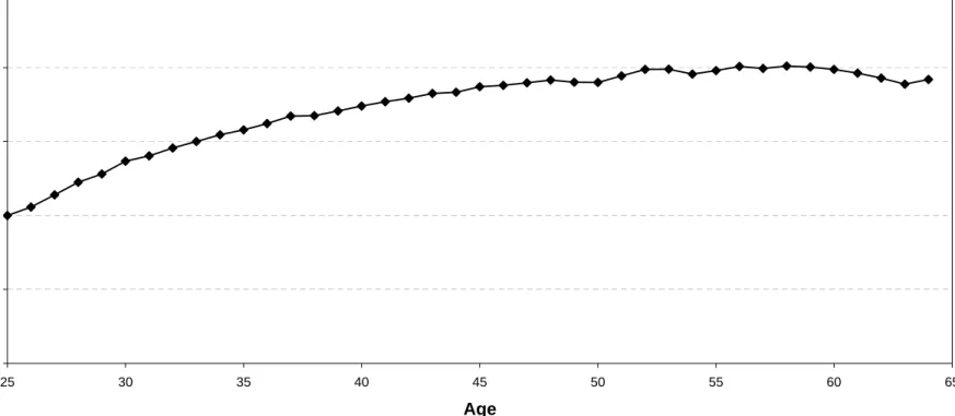
We consider a benchmark model with only permanent shocks as well as a full model with all three stochastic components. The parameters are set to estimates from Kaplan (2007). A one standard deviation permanent shock leads to about a 24 percent permanent change in wages, whereas a one standard deviation innovation to the persistent component changes wages by about 14 percent. The persistent shock is set to zero for each agent at the beginning of the working life cycle. The deterministic wage component μj is given in Figure 3. This component implies that wages approximately double over the life cycle. We approximate each productivity process with a discrete number of shocks.16
The period utility function in the model is additively separableu(c, l) = c(1−(1−νν))+φ(1−(1−l)(1γ−γ) ). Utility function parameters are set equal to Kaplan’s estimates. The coefficient of relative risk aversion is ν = 1.66. The coefficient γ = 5.55 governs the Frisch elasticity of labor (i.e.
labor = γ1(1−ll) so that the Frisch elasticity is 0.27 evaluated at l =.4). These values lie well
within a range of values estimated in the literature based upon micro-level consumption and labor data - see Browning, Hansen, and Heckman (1999). The value φ = 0.13 is the mean value estimated by Kaplan.
One important restriction on the utility function u(c, l) is the assumption of additive separability. Much of the literature on dynamic contract theory with a labor decision employs this assumption. We make use of this assumption when we design a procedure to compute solutions to the planning problem.17
The parameters of the model tax-transfer system are set to capture features of social security and federal income taxation in the U.S. Thus, the social security tax rateτ is set to equal 10.6 percent of earnings. This is the combined employee-employer tax for the old-age and survivor’s insurance component of social security. The social security benefit function
b(x) and the income tax function Tjinc are given by Figure 1 and Figure 2, which were
16We approximate the permanent component with 5 equally-spaced points in logs on the interval
[−σ12/2−3σ1,−σ21/2 + 3σ1]. Following Tauchen (1986), probabilities are set to the area under the nor-mal distribution, where midpoints between the approximating points define the limits of integration. The persistent component is approximated with 3 equally-spaced points on the interval [−4σ2,4σ2]. Transition probabilities are calculated following Tauchen (1986). The temporary component is approximated with 2 values.
17It is used in Theorem A1 in the Appendix to establish which incentive constraints bind and to reduce
discussed in the previous section.
The model is explicitly a partial equilibrium model in that wage w per efficiency unit of labor and the real interest rater are exogenous. They do not vary as we consider alternative social insurance arrangements. Nevertheless, we choose the value of the agent’s discount factor β so that a steady state of a general equilibrium version of the full model produces the interest rate r =.042 in Table 1. This interest rate is the average of the real return to stock and to long-term bonds over the period 1946-2001 (see Siegel (2002, Tables 1-1 and 1-2)). The value of the wage w in the model is then set to the value consistent with the factor inputs that produce this real return as explained in the Appendix.18
Figure 4 displays the evolution of the variance of (log) wages, earnings, work hours and consumption within the full model. The dispersion in wages early in life reflects the sum of the permanent and temporary components of productivity. The rise in wage dispersion with age reflects the role of persistent shocks. The dispersion in earnings over the life cycle closely mimics the pattern for wages. One reason for this is that, absent preference heterogeneity, the model produces little dispersion in work hours. The rise in consumption dispersion over the life cycle reflects mainly the role of persistent shocks. The levels of consumption, earnings and wage dispersion are lower at all ages within the full model compared to the U.S. facts documented in Heathcote, Storesletten, and Violante (2005). This is because Kaplan (2007) analyzes residual dispersion - dispersion after controlling for observable sources of variation such as those related to differences in education - rather than total dispersion. Although the estimate of the permanent wage shock variance is reduced compared to the estimates in Heathcote et al. (2008), the parameters related to persistent and temporary shocks are not greatly affected.
18The notion of a steady state and how to compute it is standard and follows Huggett (1996). This involves
choosing an aggregate production function and setting factor prices to marginal products. The Appendix describes in detail how this is carried out.
IV. Analyzing Welfare Gains
This section analyzes welfare gains within the permanent-shock model.
A. Maximum Welfare Gains
The maximum welfare gain to improved insurance is measured by the percentage increase
α in consumption in the allocation (cus, lus) solving the U.S. social insurance problem so that ex-ante expected utility is the same as in an allocation (cpp, lpp) solving the planning problem.19 These allocations use the same expected present value of resources. This calcu-lation is shown below. The results of this section are based on computing solutions to each problem. Computational methods are described in the Appendix.
E J j=1 βj−1u(cus j (1 +α), lusj ) =E J j=1 βj−1u(cpp j , lppj ) ≡Vpp
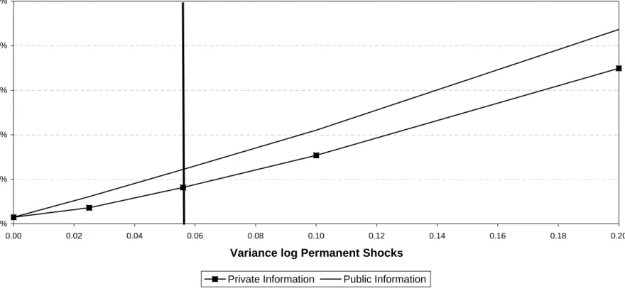
Figure 5 highlights the maximum welfare gains attainable for a range of values of the variance of the permanent component of wage shocks. Figure 5 shows that the welfare gain is increasing in this variance. This is true both when the model social insurance system only includes social security and when the model social insurance system includes both social security and income taxation.
To quantify the size of the maximum welfare gain, we need an estimate of this variance. Kaplan (2007) estimates that σ12 =.056 for permanent shocks. Thus, a one standard devia-tion shock increases wages permanently over the lifetime by about 24 percent. Heathcote et al. (2008) estimate a wage process with a similar structure to Kaplan (2007) but find that
σ2
1 =.109. One reason for this difference is that in a first stage regression Kaplan controls
for permanent differences in wages related to education whereas Heathcote et al. do not. It is valuable to keep both estimates in mind in viewing Figure 5a. Using Kaplan’s estimate,
19When the range of the period utility function of consumption is not bounded from above, then there
is always a value α solving this equation. The utility to consumption is bounded above by zero for the period utility function in Table 1. Nevertheless, as Figure 4 highlights,αis well defined for all the examples analyzed.
Figure 5a shows that the maximum welfare gain in the model of the combined social security and income tax system is equivalent to a 4.1 percent increase in consumption each period.
The analysis in Figure 5a is based upon the idea that while earnings are publicly observed both individual hours of work and individual wage rates are only privately observed. This implies that any mechanism determining consumption and labor over the lifetime must respect the incentive compatibility constraints. Figure 5b describes how important private information is for limiting the size of the gains to superior insurance. Figure 5b plots the maximum welfare gain in the economy with social security and income taxation when wage rates are private information and when they are public information. At the value σ21 =.056, the maximum welfare gain under public information is equivalent to a 6.1 percent change in consumption at each age. This gain is achieved by having all agents of a given age consume the same amount despite large differences in earnings across agents with different productivities.
The remainder of section 4 develops an understanding of what lies behind the patterns in Figure 5. In doing so, the following questions are addressed: (1) How do patterns of lifetime taxation differ in the two problems?, (2) To what degree can welfare be improved by reallocating consumption, fixing the labor allocation?, (3) How do marginal rates of substitution in the model insurance system differ from those in the planning problem? and (4) Why does the welfare gain increase as the shock variance increases?
B. Patterns of Lifetime Taxation
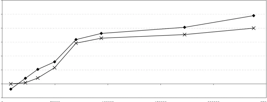
To get a preliminary idea of the economics behind the maximum welfare gains, it is useful to examine patterns of lifetime taxation. Figure 6 graphs the present value of earnings and consumption for agents at each of the five values of the permanent shock. This is done both in the model social insurance system and in the planning problem for the benchmark variance of σ12=.056. Figure 6 shows that lifetime taxation is progressive in both allocations in that the ratio of the present value of consumption to the present value of earnings falls as lifetime earnings increase. Furthermore, there is much more progression in lifetime average tax rates in the planning allocation than in the allocation under the model social insurance system. One additional feature of Figure 6 is that both allocations involve extracting resources in
present-value terms from a cohort. This last point is clear as the lifetime tax patterns under the model social insurance system is below the 45 degree line for agents at all permanent shock levels.20
A quick look at Figure 6 reveals that the labor allocation must be quite different across these two allocations as the present value of earnings differs sharply. To highlight this, we plot work time over the life cycle. Figure 7 shows that in the planning problem the highest productivity shock agents work the greatest fraction of time and the lowest productivity shock agents work the least. In the model social insurance system this pattern of work time is exactly reversed.
One issue raised by Figures 6 and 7 is the extent to which the maximum welfare gains arise from simply reallocating consumption across agents with different permanent shocks, holding the labor allocation fixed. The remaining gains are related to changing work time. Thus, if it were possible to raise the consumption of low shock agents and lower that of high shock agents, how far would such a reallocation go to improving welfare? While such a reallocation would improve ex-ante utility because the utility function is concave in consumption, this reallocation can only be pushed up to the point where the incentive constraints bind.
To answer this question, we calculate the new allocation (c∗, lus) which maximizes ex-ante utility, holding labor fixed at lus, while imposing incentive compatibility and the present value resource constraint. We find that at the benchmark valueσ2 =.056 the new allocation (c∗, lus) increases welfare over (cus, lus) by 2.9 percent, compared to a maximum 4.09 percent achieved in the planning problem. Thus, important parts of the maximum welfare gain are due both to reallocating consumption and changing the labor allocation.
C. Analyzing Wedges
We now try to better understand the sources of the welfare gains documented in Figure 5. To do so, we focus on the wedges between marginal rates of substitution and transformation. One wedge is the intratemporal wedge between the consumption-leisure marginal rate of
20Intuitively, a pay-as-you-go social security system alone should extract resources from current and future
birth cohorts to pay for “free” benefits to previous cohorts. Fullerton and Rogers (1993, Table 4-14) calculate that lifetime average tax rates in the U.S. are roughly progressive in lifetime income and that resources are extracted in present-value terms from the cohorts they analyze.
substitution and the agent’s wage. The other wedge is the intertemporal wedge between the marginal rate of substitution of consumption intertemporally and the gross interest rate. We will see shortly that the differences in work hours across the two problems turn out to be related to the differences in the intratemporal wedge.
Consider first the social insurance problem. The income tax system causes the marginal rate of substitution of consumption intertemporally to be below the gross interest rate. In fact, the progressivity of the income tax system, previously documented in Figure 2, implies that within the model the intertemporal wedge is greatest for high productivity agents. These are the agents who end up receiving high incomes.
Consider next the intratemporal wedge. Figure 8 graphs the ratio of the intratemporal marginal rate of substitution to the agents wage for each value of the permanent shock.21 Any deviation of this ratio from unity will be labeled a wedge.
Within an age group, Figure 8 shows that this wedge increases as an agent’s wage and productivity increases. The wedge is smallest for low productivity agents for two reasons. First, these agents have relatively low incomes and marginal income tax rates are relatively low at low income levels. Second, the nature of the social security system implies that at any age the marginal tax rate on additional earnings arising from social security increases as an agent’s productivity shock increases.
This second point merits some discussion. The marginal tax rate mentioned above equals the social security tax rateτ less the present value of marginal social security benefits incurred from an extra unit of earnings. This applies to agents who are below the maximum taxable earnings level. This second component differs across agents within the same age group. The reason is that agents in the model will anticipate ending up on different sections of the social security benefit function. High productivity agents will end up on the flat part of the social security benefit function and thus will incur a low marginal benefit in present value. The situation is reversed for low productivity agents as they will end up on the steep part of the benefit function. This reasoning implies that marginal tax rates arising from social security increase with productivity within the model.22
21Recall from section 3 that the wage rate in the permanent-shock model iswω(s, j) =wμjexp(s1) and
that there are five equally-spaced shock valuess11< s12< ... < s15.
We now analyze the nature of wedges that arise in a solution to the planning problem. Solutions to the planning problem will involve some incentive compatibility constraint bind-ing. As a consequence, at a solution it will not be true that all marginal rates of substitution are equated to marginal rates of transformation.
While there is an intertemporal wedge in the model social insurance problem arising from the income tax there is no intertemporal wedge in a solution to the planning problem. This difference accounts for some of the welfare gains. To see why there is no intertemporal wedge in the planning problem, assume that there is a solution with a wedge. If so, then it is possible to deliver both the same expected utility and the same ex-post utilities at lower expected present value cost, without changing the labor allocation. This can be done by eliminating the intertemporal wedge. The extra resources saved can then be used to make a uniform increase in utility to agents receiving all shocks while preserving incentive compatibility.23
Now consider the intratemporal wedge. The intratemporal marginal rate of substitution will differ from an agent’s wage rate in a solution to the planning problem depending on which incentive constraints bind. It turns out that only the local downward incentive con-straints hold with equality in a solution. These concon-straints require that an agent with a given permanent shock weakly prefers his/her own allocation to the allocation received by pretending to have the next lowest shock. An important consequence of this (see Theorem A1 in the Appendix) is that the marginal rate of substitution between consumption and labor is then strictly below the wage rate wω(s, j) in all periods for all agents except the agent receiving the highest shock.24 For the agent with the highest shock, there is no gain to distorting the consumption-labor margin at any age. The reason is that no other agent envies the consumption and output allocation of this agent. All other agents get strictly lower lifetime utility by pretending to be the high shock agent and allocating enough labor
security system varied with age for a median productivity agent. Early in life the marginal tax rate is slightly below τ = .106. It decreases with age but remains positive at all ages. Broadly, our results are similar to the marginal social security tax rates calculated by Feldstein and Samwick (1992, Table 1).
23Rogerson (1985) and Golosov, Kocherlakota, and Tsyvinski (2003) present a necessary condition on this
margin in planning problems with a more general structure of shocks. Their main result is the “inverse” Euler equation. The result stated in the text is a special case of their result as the inverse Euler equation reduces to the claim made above, absent period-by-period shocks. With period-by-period shocks, a solution to the planning problem will have an intertemporal wedge.
time to produce the higher output required.
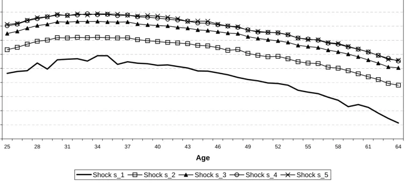
Next, we examine the size of the intratemporal wedge. Figure 9 graphs the ratio of the marginal rate of substitution to the agent’s wage rate at each age for each of the five possible values of the permanent shock. Figure 9 shows that the intratemporal wedge is positive for all agents with the exception of the agent with the highest permanent shock. Furthermore, within an age group the magnitude of this wedge decreases as an agent’s wage increases.
In the context of the permanent-shock model, we are not aware of any existing theoretical result which describes how the wedge at each age moves as productivity increases. However, for the static Mirrlees model there are theoretical and computational results (see, for example, Tuomala (1990), Saez (2001) and the references cited in these papers). In the Mirrlees model, the lognormal distribution of productivity is important for wedges to decline as productivity increases. We have computed the nature of wedges in the permanent-shock model when we replace the lognormal distribution with a Pareto distribution. The literature has argued that the upper tail of the earnings distribution has fat tails which are more in line with a Pareto distribution. For the Pareto distribution with the same mean and variance, we find that wedges do not decrease as productivity increases.25
We conjecture that the differences in wedges and the differences in lifetime taxation are the key reasons why the maximum welfare gains increase as labor productivity risk increases. There is too little progression in lifetime taxation in the model social insurance system compared to the planners problem as risk increases. Furthermore, the intratemporal wedge on high productivity agents typically increases as risk increases in the model social insurance system whereas the wedge on the highest productivity agents within an age group is always zero in the planning problem.
25Following Tauchen (1986), we approximate a Pareto distribution with five equally-spaced points one
standard deviation apart. The resulting wedge is positive and displays little variation across ages. The wedge for the lowest four shock levels averages approximately .12, .10, .16 and .20, in order of increasing productivity. The wedge for the highest productivity level is approximately zero in computations.
V. Reforming the Social Insurance System
We examine two ways to reform the model social insurance system. Reform 1 is a piece-meal reform in which a component of the social insurance system is changed while maintain-ing the remainder of the system. In Reform 1 we change the social security benefit function without changing income taxation or the social security tax rate. Reform 2 is a radical reform as social security and income taxation are eliminated and are replaced with a tax on the present value of earnings.
Reform 1 and 2 are optimal parametric reforms. In each case we search over the parameters of the respective tax functions to find the parameter vector which maximizes ex-ante expected utility of the cohort of agents.26 In each reform the same present value of resources is extracted from the cohort as in the original social insurance system. The Appendix describes computational methods. The Appendix is also useful for understanding how to achieve a tax on the present value of earnings using a period-by-period tax system. We note that a present-value tax is compatible with the provision of retirement benefits as such a tax can be achieved with very different timings of taxes and transfers over the lifetime.
A. Motivation
The policy literature is full of discussions of piecemeal reforms. In the social security literature, it is common to find the suggestion that the value of marginal social security benefits incurred by extra earnings should be more closely linked with marginal taxes paid in order to improve efficiency or a welfare measure. These considerations motivate the analysis of Reform 1 which is an optimal piecemeal reform that flexibly changes the benefit function.
The motivation for Reform 2 is that it is simple and that there are reasons to think that it might work well within the permanent-shock model. Within the permanent-shock model, a present-value tax has two important properties. First, it imposes no intertemporal wedge. Second, it imposes an age-invariant wedge on the intratemporal margin that can be made to
26Our analysis of optimal parametric reforms is similar in some respects to the work of Conesa, Kitao, and
Krueger (2009). They choose the parameters of a labor income tax function and a linear capital income tax to maximize ex-ante lifetime utility in steady state.
flexibly differ across agents.27 The previous section argued that the first property holds in a solution to the planning problem and that the second property is approximately supported in computations.
B. Analysis
The welfare gain to each reform is given in Table 2. Welfare gains are stated in terms of the permanent percentage increase in consumption in the allocation in the model without the reform which is equivalent to the expected utility delivered under the optimal reform. Welfare gains are calculated for both the full model (i.e the model with permanent, persistent and temporary shocks) and the permanent-shock model.
Table 2: Welfare Gains to Optimal Parametric Reforms
We first discuss the results for the permanent-shock model. For Reform 1, we calculate the best constant benefit, the best linear benefit and the best quadratic benefit as a function of average lifetime earnings. The best constant benefit function in the permanent-shock model leads to a welfare gain of 0.14 percent. A constant social security benefit increases the progressivity of lifetime earnings taxation but also increases marginal earnings taxes across earnings levels. The best linear benefit function has a positive intercept and a negative slope and leads to a welfare gain of 0.18 percent. The best quadratic benefit function that we find does not improve welfare over the best linear function. This class of reforms achieves only a small fraction of the maximum possible welfare gain. This occurs because these reforms are poorly focused: greater progression in lifetime taxation is achieved by imposing an even larger intratemporal wedge on high productivity agents and the change in the benefit function does not eliminate the wedge on the intertemporal consumption margin.
In contrast, an optimal present-value tax leads to a large welfare gain worth a 3.95 percent increase in consumption. We obtain this result when the class of tax functions are increasing
27Werning (2007) shows that a present-value tax system is optimal in some contexts. Specifically, he
shows that such a tax implements a solution to a planning problem in the context of an infinitely-lived agent model where labor productivity takes on two possible values, labor productivity is private information and preferences are of the constant Frisch elasticity of labor form.
step functions. This reform achieves nearly all of the maximum possible welfare gain in the permanent-shock model.
We highlight two reasons why the optimal present-value earnings tax works well in the permanent-shock model. First, it allows for a flexible choice of lifetime taxation. Indeed, the graph of the present value of consumption as a function of the present value of earnings which turns out to be optimal is essentially the pattern in the planning problem - previously displayed in Figure 6. Second, the present-value tax is able to closely approximate the pattern of intratemporal and intertemporal wedges found in a solution to the planning problem.28
We now discuss results for the full model. For Reform 1, the best constant, linear, and quadratic benefit functions lead to gains worth a 0.56,1.07 and 1.15 percent increase in consumption, respectively. The best quadratic benefit function has a positive intercept, but negative values for the coefficients on the slope and quadratic terms. Thus, the piecemeal reform that maximizes ex-ante welfare does not involve more closely linking the value of marginal benefits received to marginal taxes paid. Greater progression in lifetime taxation is achieved within this reform by increasing intratemporal wedges. For Reform 2 we find that in the full model the best present-value tax that is within the piecewise-linear class leads to a small welfare loss equivalent to a 0.07 percent decrease in consumption. Thus, even though a present-value tax is both a simple and well-focused reform within the permanent-shock model, this class of reforms does not lead to welfare gains within the richer idiosyncratic shock structure of the full model.
To get some insight into what is behind these results, we first examine the pattern of lifetime taxation. Figure 10 shows that the progression in lifetime taxation is greater in Reform 1 and Reform 2 than in the benchmark model.29 Moreover, the pattern of lifetime
28At a deeper level, a present-value tax may work well within these economies for two quite different
reasons. First, one might conjecture that interior solutions to the planning problem with (i) constant Frisch elasticity of labor preferences (i.e. u(cj, lj) = u(cj) +φl
1+γ j
1+γ) and (ii) permanent proportional productivity
differences have the property that only local downward incentive constraints bind. If so, such allocations can always be implemented by a present-value tax system. A key property of such a solution, given assumptions (i)-(ii), is that the intratemporal wedge is age invariant - see the proof of Theorem A1(iii) in the Appendix. Second, the preferences used in Table 1 may effectively be close to those with constant Frisch elasticity of labor.
29The 10th, 50th and 90th percentile of the present value of earnings distribution in the benchmark model
taxation is broadly similar in both reforms over much of the domain. So the difference in welfare gain between Reform 1 and Reform 2 does not seem to come from differences in this measure of tax progression. The optimal present-value tax function in Reform 2 is roughly linear over most of the domain but is eventually flat well past the 99th percentile of the distribution - this occurs at a present value of earnings equal to 45.
We now describe how the reforms impact consumption. Both reforms produce a downward shift in the distribution of the present value of earnings compared to the benchmark model. The result is that mean consumption at almost all ages is lower in both reforms than in the benchmark model but, perhaps surprisingly, only Reform 1 substantially reduces measures of the dispersion in consumption at all ages compared to the benchmark model. This implies that the component of expected utility due to consumption is slightly lower in Reform 1 compared to the benchmark model but is even lower in Reform 2 compared to Reform 1 or to the benchmark model.
Next we describe how the reforms impact work hours. Reform 1 reduces the mean hours of work at all ages compared to the benchmark model and it produces about the same coefficient of variation in hours at all ages. Thus, the ex-ante utility from leisure is greater in Reform 1 than in the benchmark model. Reform 2 reduces mean hours of work at all ages below that in the benchmark model and below that in Reform 1. However, Reform 2 nearly doubles the coefficient of variation of hours early in the life cycle compared to the benchmark model. The overall effect of Reform 2 is to increase the ex-ante utility from leisure compared to the benchmark model. Both reforms increase the correlation between work hours and labor productivity at all ages compared to the benchmark model. Figure 10 suggests that different income effects on high and low lifetime earnings agents is partly behind the increase in correlation. This increase in correlation is a key part of the mechanism within the permanent-shock model for achieving the maximum possible welfare gain.
We now consider Reform 3 to determine if an important part of the welfare gain obtained by Reform 2 in the permanent-shock model comes simply from eliminating capital income taxation and the associated intertemporal wedge. Reform 3 is a piecemeal reform that maintains social security and income taxation but exempts capital income from entering into taxable income. An additional proportional labor income tax is added to satisfy the
present-value resource constraint. Eliminating capital income taxation in this way produces a welfare gain of 0.22 percent in the permanent-shock model and a welfare loss of −0.22 percent in the full model. Thus, simply eliminating intertemporal wedges in this crude way, without substantially increasing the progressivity of lifetime taxation or altering the pattern of intratemporal wedges, does not go very far towards producing the maximum welfare gain in the permanent-shock model.
All of the analysis in the paper is based upon the assumption that factor prices are fixed and do not change as the social insurance system is changed. We now take a step towards determining how a closed-economy analysis might differ by simply calculating how the aggregate capital and labor evolve over time at fixed factor prices within the full model. We assume that each reform applies only to each successive cohort of newborn agents and that all other agents who are alive at the start of the reform face the original social insurance system. The original social insurance system was calibrated to be consistent with a steady state in the full model with no government debt. We view any change in the capital-labor ratio over time as reflecting a need for factor prices to adjust in a closed-economy analysis. An increase in the ratio is viewed as a force which depresses the interest rate and raises the wage rate.
In Reform 1 the capital-labor ratio changes by well under one percent over the first 40 periods. In contrast, Reform 2 and 3 show much larger movements. After 40 periods this ratio falls by 10 percent in Reform 2 and increases by 18 percent in Reform 3. This is due almost entirely to the movement in the numerator - total asset holdings less government debt. We conjecture that little of the welfare gains we find for Reform 1 would vanish in a closed-economy analysis simply because the large effects at the individual level wash out almost entirely for factor inputs both within age group and at the aggregate level. It is less clear whether or not the results for Reform 2 and 3 would continue to hold.
In closing this section, we think that finding parametric tax systems that work well within the full model is a useful problem. This problem connects the policy literature to the literature on optimal taxation. We acknowledge that the tax systems that we have explored can be improved upon as both reforms violate the inverse Euler equation which is a necessary
condition on the intertemporal margin for a solution to the planning problem.30 Further theoretical and computational work that give insight into wedges arising in planning problems would be useful for finding parametric tax systems that produce larger welfare gains.
30Rogerson (1985) and Golosov et al. (2003) present the inverse Euler equation result. Kocherlakota
VI. Conclusion
The question of whether to or how to fundamentally redesign social security systems has been and continues to be a major policy issue in the U.S. and in many other countries. One’s position on this issue is likely to depend upon one’s view of the rationale for social security and for social insurance more broadly. One standard rationale is the provision of insurance for risks that are not easily insured in private markets.
We provide a quantitative analysis of the U.S. social insurance system within a framework with important idiosyncratic, labor-market risks. We find that large welfare gains to changing the social insurance system are possible. Systems that can achieve such welfare gains need not be more complicated than the current U.S. system. Specifically, we find that an optimal tax on the present value of earnings does this within the model with only permanent shocks and that changing only the social security benefit function does this within the model with permanent, persistent and purely temporary productivity shocks of the nature found in U.S. wage rate data. These results are based upon maximizing ex-ante utility for a cohort. Thus, the objective reflects an insurance role both for productivity differences present at the start of the working lifetime as well as for productivity shocks occuring throughout the working lifetime.
We mention three directions to pursue in future work. First, it would be valuable to know quantitative properties of the solution to the planning problem within the full model. This would require important theoretical and/or computational advances.31 Second, this paper treats labor productivity as being unaffected by the social insurance system. We expect that human capital models (e.g. Huggett, Ventura, and Yaron (2007)) will be central both as positive models of inequality and as models for the analysis of social insurance issues. Because skill acquisition responds to policy in human capital models, labor productivity will not be policy invariant. Whether the gains to adopting superior systems are even larger within such models is an open question. Third, future work might expand the analysis of the social insurance system to go beyond income taxation and social security as well as provide a closed-economy analysis to complement the open-economy analysis pursued in this work.
31Fernandes and Phelan (2000) provide a recursive formulation of a planning problem with persistent
Appendix A
The Appendix contains two sections. Section A.1 describes our methods for computing solutions to the planning problem, the social insurance problem and the parametric planning problems. Section A.2 proves Theorem A1. In the Appendix the labor-productivity function is sometimes set to ω(sj, j) =sj solely to shorten and simplify expressions. FORTRAN programs that compute solutions to all the problems analyzed in the paper are available upon request.
A.1. Computation
A.1.1. Social Insurance Problem
The social insurance problem is stated below as a dynamic programming problem. This involves re-formulating the present value budget constraint as a sequence of budget constraints where resources are transferred across periods with a risk-free asset. Risk-free asset holding must then always lie above period and shock specific borrowing limitsaj(s) consistent with solvency at the terminal age. The state variable is x = (a, s, z), where a is asset holdings, s is the period shock vector determining productivity and z is average past earnings. The functionsTj andFj describe the tax system and the law of motion for average past earnings. The shock is Markovian with transition probabilityπ(s|s).
Vj(a, s, z) = max(c,l,a)u(c, l) +βsVj+1(a, s, z)π(s|s)
(1)c+a≤a(1 +r) +wω(s, j)l−Tj(x, wω(s, j)l) (2)c≥0, a≥aj(s);l∈[0,1]
(3)z=Fj(z, wω(s, j)l)
This problem is solved computationally by backwards induction. The value function Vj is computed at selected grid points (a, s, z) by solving the right-hand-side of Bellman’s equation. We use the simplex method (see Press et al (1994)). Evaluating the right-hand-side of Bellman’s equation involves a bi-linear interpolation of the functionVj+1(a, s, z) over the asset and average past earnings dimensions: (a, z). We set the borrowing limit to a fixed valueain each period. We then relax this value so that it is not binding. This is a device for imposing period and state specific limitsaj(s). To use this device, penalties are imposed for states and decisions implying negative consumption.32
We compute ex-ante, expected utility Vus and the expected cost, denoted Cost, of running the social insurance system by simulation, under the assumption that an agent starts out with no assets. Specifically, we draw a large number (100,000) of lifetime labor-productivity profiles, compute realized utility and realized cost for each profile, using the computed optimal decision rules, and then compute averages. The same 100,000 histories are used in the calculation of expected utility and expected cost in the analysis of reforms.
A.1.2. Steady State Calibration
We calibrate the discount factor β using the algorithm below. This algorithm is based on computing a stationary equilibrium. To set up this framework, we assume that (i) there is an aggregate production
32The backward induction procedure takes as given a value for average earnings in the economy. This
value is used to determine the tax function Tj. Thus, an additional loop is needed so that guessed and implied values of average earnings coincide.
functionY =F(K, L) =KαL1−α stated in terms of aggregate capitalK and laborL, (ii) physical capital depreciates at rateδ and (iii) population growth isn.
We define an equilibrium using the recursive language - see Huggett (1996). To keep track of agent heterogeneity, we use probability measures ψj to describe the fraction of age j agents that have a state vector x = (a, s, z) lying in particular subsets of the state space X. The relative size of different age cohorts is given by φj, where φj+1 = φj/(1 +n) and jφj = 1. Denote aggregate capital, labor and government spending and consumption (K, L, G, C): K ≡jφj adψj,L≡jφj ω(s, j)l(x, j)dψj and C≡jφjc(x, j)dψj. The probability measures must be consistent with one another. This is captured by the recursionψj+1= Γj(ψj), where Γj(ψj)(·)≡ P(x, j,·)dψj, andP is a transition function induced by the transition probabilities on shocks and by the periodj decision rules. We do not write down all the details associated with the construction of this transition function partly because the algorithm below calculates the relevant integrals by simulating a large number of histories rather than by calculating probability measures on a rich collection of subsets of the state space and then integrating. However, details of how to do so are in Huggett (1996).
Definition: A stationary equilibrium is (c(x, j), l(x, j), a(x, j), w, r, G), tax-transfer functions (T1, ..., TJ) and probability measures(ψ1, ..., ψJ)such that
1. (c,l,a) solve Bellman’s equation (Appendix A.1.1), given(w, r)and Tj. 2. w=F2(K, L)and r=F1(K, L)−δ 3. ψj+1= Γj(ψj),∀j 4. G=jφjTj(x, wω(s, j)l(x, j))dψj 5. C+K(n+δ) +G=F(K, L) Algorithm: 1. Fix (α, δ, n) = (.33, .06, .01).
2. Set r=.042 andw= 1.19461. Given (r, α, δ), equilibrium condition 2 pins down the wagew at the value stated and pins down the capital-labor ratioK/L.
3. Guess the discount factor and average earnings (β,¯e).
4. Compute decision rules (c, l, a) solving Bellman’s equation, given the information in steps 1-3 using the procedures described in Appendix A.1.1.
5. Calculate implied values of aggregates (K, L,¯e,jφjTj(x, wω(s, j)l(x, j))dψj) via simulation us-ing the decision rules.
6. If K/L = K/L, ¯e = ¯e and jφjTj(x, wω(s, j)l(x, j))dψj > 0, then stop. Otherwise, update (β,¯e) and repeat steps 4-5.
Comments:
1. We computeβfor the full model at the parameters listed in Table 1 and fix this value for all subsequent analysis.
2. The initial value of β in step 3 is set to β = 1/(1 +r). In carrying out this algorithm we first adjust average earnings ¯e in steps 3-6 until ¯e = ¯e. The value of β is increased until step 6 approximately holds. We choose ¯ein step 3 because the tax-transfer function is only specified once ¯eis known - see section 2.4.1.