Fractals, topology, complex arithmetic and fascinating computer graphics.

(1)

Mandelbrot Set

Fractals, topology, complex arithmetic and fascinating computer graphics.

Benoit Mandelbrot was a Polish/French/American mathematician who has spent most of his career at the IBM Watson Research Center in Yorktown Heights, N.Y. He coined the termfractal and published a very inﬂuential book,The Fractal Geometry of Nature, in 1982. An image of the now famous Mandelbrot set appeared on the cover ofScientiﬁc Americanin 1985. This was about the time that computer graphical displays were becoming widely available. Since then, the Mandelbrot set has stimulated deep research topics in mathematics and has also been the basis for an uncountable number of graphics projects, hardware demos, and Web pages.

To get in the mood for the Mandelbrot set, consider the region in the complex plane of trajectories generated by repeated squaring,

zk+1=z2k, k= 0,1, ...

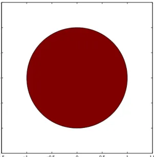
For which initial values z0 does this sequence remain bounded as k → ∞? It is easy to see that this set is simply the unit disc, |z0| <= 1, shown in ﬁgure 13.1. If |z0| <= 1, the sequence zk remains bounded. But if |z0| > 1, the sequence is

unbounded. The boundary of the unit disc is the unit circle, |z0| = 1. There is nothing very diﬃcult or exciting here.

The deﬁnition is the Mandelbrot set is only slightly more complicated. It involves repeatedly adding in the initial point. The Mandelbrot set is the region in the complex plane consisting of the valuesz0 for which the trajectories deﬁned by

zk+1=z2k+z0, k= 0,1, ...

remain bounded at k → ∞. That’s it. That’s the entire deﬁnition. It’s amazing that such a simple deﬁnition can produce such fascinating complexity.

Copyright c⃝2011 Cleve Moler

Matlab⃝R is a registered trademark of MathWorks, Inc.TM

October 2, 2011

(2)

−1.5 −1 −0.5 0 0.5 1 1.5 −1.5 −1 −0.5 0 0.5 1 1.5

Figure 13.1. The unit disc is shown in red. The boundary is simply the unit circle. There is no intricate fringe.

−2 −1.5 −1 −0.5 0 0.5 1 −1.5 −1 −0.5 0 0.5 1 1.5

Figure 13.2. The Mandelbrot set is shown in red. The fringe just outside the set, shown in black, is a region of rich structure.

(3)

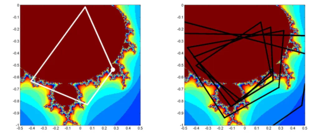
Figure 13.3. Two trajectories. z0 = .25-.54i generates a cycle of length four, while nearby z0 = .22-.54i generates an unbounded trajectory.

Figure 13.2 shows the overall geometry of the Mandelbrot set. However, this view does not have the resolution to show the richly detailed structure of the fringe just outside the boundary of the set. In fact, the set has tiny ﬁlaments reaching into the fringe region, even though the fringe appears to be solid black in the ﬁgure. It has recently been proved that the Mandelbrot set is mathematically connected, but the connected region is sometimes so thin that we cannot resolve it on a graphics screen or even compute it in a reasonable amount of time.

To see how the deﬁnition works, enter

z0 = .25-.54i z = 0

into_Matlab. Then use the up-arrow key to repeatedly execute the statement

z = z^2 + z0

The ﬁrst few lines of output are

0.2500 - 0.5400i 0.0209 - 0.8100i -0.4057 - 0.5739i 0.0852 - 0.0744i 0.2517 - 0.5527i ...

The values eventually settle into a cycle

0.2627 - 0.5508i 0.0156 - 0.8294i -0.4377 - 0.5659i 0.1213 - 0.0446i

(4)

0.2627 - 0.5508i ...

This cycle repeats forever. The trajectory remains bounded. This tells us that the starting value value, z0 = .25-.54i, is in the Mandelbrot set. The same cycle is shown in the left half of ﬁgure 13.3.

On the other hand, start with

z0 = .22-.54i z = 0

and repeatedly execute the statement

z = z^2 + z0

You will see

0.2200 - 0.5400i -0.0232 - 0.7776i -0.3841 - 0.5039i 0.1136 - 0.1529i 0.2095 - 0.5747i ...

Then, after 24 iterations,

... 1.5708 - 1.1300i 1.4107 - 4.0899i -14.5174 -12.0794i 6.5064e+001 +3.5018e+002i -1.1840e+005 +4.5568e+004i

The trajectory is blowing up rapidly. After a few more iterations, the floating point numbers overflow. So thisz0 is not in the Mandelbrot set. The same unbounded trajectory is shown in the right half of figure 13.3. We see that the first value,

z0 = .25-.54i, is in the Mandelbrot set, while the second value,z0 = .22-.54i, which is nearby, is not.

The algorithm doesn’t have to wait untilzreachs floating point overflow. As soon aszsatisfies

abs(z) >= 2

subsequent iterations will essential square the value of|z| and it will behave like 22k.

Try it yourself. Put these statements on one line.

z0 = ... z = 0; while abs(z) < 2 z = z^2+z0; disp(z), end

(5)

Use the up arrow and backspace keys to retrieve the statement and changez0 to diﬀerent values near .25-.54i. If you have to hit <ctrl>-c to break out of an inﬁnite loop, thenz0is in the Mandelbrot set. If thewhilecondition is eventually

falseand the loop terminates without your help, thenz0is not in the set. The number of iterations required forzto escape the disc of radius 2 provides the basis for showing the detail in the fringe. Let’s add an iteration counter to the loop. A quantity we calldepthspeciﬁes the maximum interation count and thereby determines both the level of detail and the overall computation time. Typical values ofdepthare several hundred or a few thousand.

z0 = ... z = 0; k = 0;

while abs(z) < 2 && k < depth z = z^2+z0;

k = k + 1; end

The maximum value of kis depth. If the value of k is less thandepth, thenz0

is outside the set. Large values of k indicate thatz0is in the fringe, close to the boundary. Ifkreachesdepththenz0is declared to be inside the Mandelbrot set.

Here is a small table of iteration counts sz0ranges over complex values near

0.22-0.54i. We have set depth = 512.

0.205 0.210 0.215 0.220 0.225 0.230 0.235 0.240 0.245 -0.520 512 512 512 512 512 512 44 512 512 -0.525 512 512 512 512 512 36 51 512 512 -0.530 512 512 512 512 35 31 74 512 512 -0.535 512 512 512 512 26 28 57 512 512 -0.540 512 139 113 26 24 73 56 512 512 -0.545 512 199 211 21 22 25 120 512 512 -0.550 33 25 21 20 20 25 63 85 512 -0.555 34 20 18 18 19 21 33 512 512 -0.560 62 19 17 17 18 33 162 40 344

We see that about half of the values are less thandepth; they correspond to points outside of the Mandelbrot set, in the fringe near the boundary. The other half of the values are equal todepth, corresponding to points that are regarded as in the set. If we were to redo the computation with a larger value ofdepth, the entries that are less than512in this table would not change, but some of the entries that are now capped at512might increase.

The iteration counts can be used as indices into an RGB color map of size

depth-by-3. The ﬁrst row of this map speciﬁes the color assigned to any points on thez0grid that lie outside the disc of radius 2. The next few rows provide colors for the points on the z0grid that generate trajectories that escape quickly. The last row of the map is the color of the points that survivedepthiterations and so are in the set.

(6)

The map used in ﬁgure 13.2 emphasizes the set itself and its boundary. The map has 12 rows of white at the beginning, one row of dark red at the end, and black in between. Images that emphasize the structure in the fringe are achieved when the color map varies cyclicly over a few dozen colors. One of the exercises asks you to experiment with color maps.

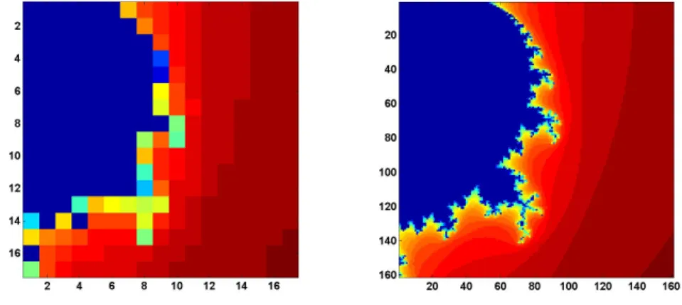
Figure 13.4. Improving resolution.

Array operations.

Our scriptmandelbrot_recapshows how_Matlabarray arithmetic operates a grid of complex numbers simultaneously and accumulates an array of iteration counters, producing images like those in figure 13.4 The code begins by defining the region in the complex plane to be sampled. A step size of0.05gives the coarse resolution shown on the right in the figure.

x = 0: 0.05: 0.80; y = x’;

The next section of code uses an elegant, but tricky, bit of_Matlab indexing known as Tony’s Trick. The quantitiesxand yare one-dimensional real arrays of lengthn, one a column vector and the other a row vector. We want to create a two-dimensionaln-by-narray with elements formed from all possible sums of elements fromxandy.

zk,j =xk+yji, i=

√

−1, k, j= 1, ..., n

This can be done by generating a vectoreof lengthnwith all elements equal to one. Then the quantityx(e,:)is a two-dimensional array formed by usingx, which is the same asx(1,:),ntimes. Similarly,y(:,e)is a two-dimensional arrray containing

(7)

n = length(x); e = ones(n,1);

z0 = x(e,:) + i*y(:,e);

If you ﬁnd it hard to remember Tony’s indexing trick, the functionmeshgrid

does the same thing in two steps.

[X,Y] = meshgrid(x,y); z0 = X + i*Y;

Now initialize two more arrays, one for the complex iterates and one for the counts.

z = zeros(n,n); c = zeros(n,n);

Here is the Mandelbrot iteration repeateddepthtimes. With each iteration we also keep track of the iterates that are still within the circle of radius 2.

depth = 32; for k = 1:depth

z = z.^2 + z0; c(abs(z) < 2) = k; end

We are now ﬁnished with z. The actual values of z are not important, only the counts are needed to create the image. Our grid is small enough that we can actually print out the countsc.

c

The results are

c = 32 32 32 32 32 32 11 7 6 5 4 3 3 3 2 2 2 32 32 32 32 32 32 32 9 6 5 4 3 3 3 2 2 2 32 32 32 32 32 32 32 32 7 5 4 3 3 3 2 2 2 32 32 32 32 32 32 32 32 27 5 4 3 3 3 2 2 2 32 32 32 32 32 32 32 32 30 6 4 3 3 3 2 2 2 32 32 32 32 32 32 32 32 13 7 4 3 3 3 2 2 2 32 32 32 32 32 32 32 32 14 7 5 3 3 2 2 2 2 32 32 32 32 32 32 32 32 32 17 4 3 3 2 2 2 2 32 32 32 32 32 32 32 16 8 18 4 3 3 2 2 2 2 32 32 32 32 32 32 32 11 6 5 4 3 3 2 2 2 2 32 32 32 32 32 32 32 19 6 5 4 3 2 2 2 2 2 32 32 32 32 32 32 32 23 8 4 4 3 2 2 2 2 2 32 32 32 19 11 13 14 15 14 4 3 2 2 2 2 2 2 22 32 12 32 7 7 7 14 6 4 3 2 2 2 2 2 2 12 9 8 7 5 5 5 17 4 3 3 2 2 2 2 2 1 32 7 6 5 5 4 4 4 3 3 2 2 2 2 2 1 1 17 7 5 4 4 4 4 3 3 2 2 2 2 2 2 1 1

(8)

We see that points in the upper left of the grid, with fairly small initialz0values, have survived 32 iterations without going outside the circle of radius two, while points in the lower right, with fairly large initial values, have lasted only one or two iterations. The interesting grid points are in between, they are on the fringe.

Now comes the ﬁnal step, making the plot. The image command does the job, even though this is not an image in the usual sense. The count values incare used as indices into a 32-by-3 array of RGB color values. In this example, thejet

colormap is reversed to give dark red as its first value, pass through shades of green and yellow, and finish with dark blue as its 32-nd and final value.

image(c) axis image

colormap(flipud(jet(depth)))

Exercises ask you to increase the resolution by decreasing the step size, thereby producing the other half of ﬁgure 13.4, to investigate the eﬀect of changingdepth, and to invesigate other color maps.

Mandelbrot GUI

Theexmtoolbox functionmandelbrot is your starting point for exploration of the Mandelbrot set. With no arguments, the statement

mandelbrot

provides thumbnail icons of the twelve regions featured in this chapter. The state-ment

mandelbrot(r)

withrbetween 1 and 12 starts with ther-th region. The statement

mandelbrot(center,width,grid,depth,cmapindx)

explores the Mandelbrot set in a square region of the complex plane with the speci-ﬁedcenterandwidth, using agrid-by-gridgrid, an iteration limit ofdepth, and the color map numbercmapindx. The default values of the parameters are

center = -0.5+0i width = 3 grid = 512 depth = 256 cmapindx = 1 In other words, mandelbrot(-0.5+0i, 3, 512, 256, 1)

generates ﬁgure 13.2, but with thejets color map. Changing the last argument from 1 to 6generates the actual ﬁgure 13.2 with the fringe color map. On my laptop, these computations each take about half a second.

(9)

grid^2 * depth

So the statement

mandelbrot(-0.5+0i, 3, 2048, 1024, 1)

could take

(2048/512)2·(1024/256) = 64

times as long as the default. However, this is an overestimate and the actual exe-cution time is about 11 seconds.

Most of the computational time required to compute the Mandelbrot set is spent updating two arrayszand kzby repeatedly executing the step

z = z.^2 + z0; j = (abs(z) < 2); kz(j) = d;

This computation can be carried out faster by writing a functionmandelbrot_step

in C and creating as a _Matlab executable or c-mex file. Different machines and operating systems require different versions of a mex file, so you should see files with names like mandelbrot_step.mexw32 and mandelbrot_step.glnx64 in the

exmtoolbox.

Themandelbrot gui turns on the_Matlabzoom feature. The mouse pointer becomes a small magnifying glass. You can click and release on a point to zoom by a factor of two, or you can click and drag to delineate a new region.

Themandelbrotgui provides several uicontrols. Try these as you read along. The listbox at the bottom of the gui allows you to select any of the predeﬁned regions shown in the ﬁgures in this chapter.

depth. Increase the depth by a factor of3/2or 4/3.

grid. Reﬁne the grid by a factor of 3/2 or 4/3. The depth and grid size are always a power of two or three times a power of two. Two clicks on the depth or

gridbutton doubles the parameter.

color. Cycle through several color maps. jets and hots are cyclic repetitions of short copies of the basic_Matlabjetandhotcolor maps. cmyk cycles through eight basic colors, blue, green, red, cyan, magenta, yellow, gray, and black. fringe

is a noncyclic map used for images like ﬁgure 13.2.

exit. Close the gui.

The Mandelbrot set isself similar. Small regions in the fringe reveal features that are similar to the original set. Figure 13.6, which we have dubbed “Mandelbrot

(10)

Figure 13.5. The ﬁgures in this chapter, and the predeﬁned regions in our mandelbrot program, show these regions in the fringe just outside the Mandelbrot set.

Junior”, is one example. Figure 13.7, which we call the “‘Plaza”, uses our flag

colormap to reveal ﬁne detail in red, white and blue.

The portion of the boundary of the Mandelbrot set between the two large, nearly circular central regions is known as “The Valley of the Seahorses”. Fig-ure 13.8 shows the result of zooming in on the peninsula between the two nearly circular regions of the set. The ﬁgure can be generated directly with the command

mandelbrot(-.7700-.1300i,0.1,1024,512)

We decided to name the image in figure 13.9 the “West Wing” because it resembles the X-wing fighter that Luke Skywalker flies in Star Wars and because it is located near the leftmost, or far western, portion of the set. The magnification factor is a relatively modest 104, sodepth does not need to be very large. The command to generate the West Wing is

mandelbrot(-1.6735-0.0003318i,1.5e-4,1024,160,1)

One of the best known examples of self similarity, the “Buzzsaw”, is shown in ﬁgure 13.11. It can be generated with

(11)

4.0e-11,1024,2048,2)

Takingwidth = 4.0e-11corresponds to a magniﬁcation factor of almost 1011_{. To} appreciate the size of this factor, if the original Mandelbrot set ﬁlls the screen on your computer, the Buzzsaw is smaller than the individual transistors in your machine’s microprocessor.

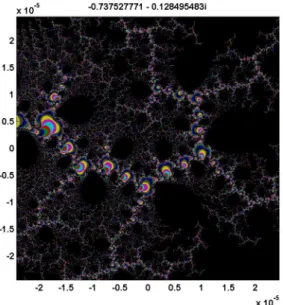
We call ﬁgure 13.12 “Nebula” because it reminds us of interstellar dust. It is generated by

mandelbrot(0.73752777-0.12849548i,4.88e-5,1024,2048,3)

The next three images are obtained by carefully zooming on one location. We call them the “Vortex”, the “Microbug”, and the “Nucleus”.

mandelbrot(-1.74975914513036646-0.00000000368513796i, ... 6.0e-12,1024,2048,2) mandelbrot(-1.74975914513271613-0.00000000368338015i, ... 3.75e-13,1024,2048,2) mandelbrot(-1.74975914513272790-0.00000000368338638i, ... 9.375e-14,1024,2048,2)

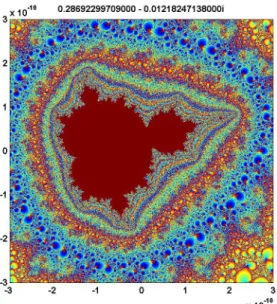
The most intricate and colorful image among our examples is ﬁgure 13.16, the “Geode”. It involves a ﬁne grid and a large value of depth and consequently requires a few minutes to compute.

mandelbrot(0.28692299709-0.01218247138i,6.0e-10,2048,4096,1)

These examples are just a tiny sampling of the structure of the Mandelbrot set.

Recap

%% Mandelbrot Chapter Recap

(12)

% introduced in the Mandelbrot Chapter of "Experiments in MATLAB". % You can access it with

%

% mandelbrot_recap % edit mandelbrot_recap % publish mandelbrot_recap %

% Related EXM programs %

% mandelbrot %% Define the region.

x = 0: 0.05: 0.8; y = x’;

%% Create the two-dimensional complex grid using Tony’s indexing trick. n = length(x);

e = ones(n,1);

z0 = x(e,:) + i*y(:,e);

%% Or, do the same thing with meshgrid. [X,Y] = meshgrid(x,y);

z0 = X + i*Y;

%% Initialize the iterates and counts arrays. z = zeros(n,n);

c = zeros(n,n);

%% Here is the Mandelbrot iteration. depth = 32;

for k = 1:depth z = z.^3 + z0; c(abs(z) < 2) = k; end

%% Create an image from the counts. c

image(c) axis image %% Colors

(13)

Exercises

13.1Explore. Use the mandelbrotgui to ﬁnd some interesting regions that, as far as you know, have never been seen before. Give them your own names.

13.2depth. Modify mandelbrot_recapto reproduce our table of iteration counts for x = .205:.005:.245 and y = -.520:-.005:-.560. First, use depth = 512. Then use larger values ofdepthand see which table entries change.

13.3Resolution. Reproduce the image in the right half of ﬁgure 13.4.

13.4Big picture. Modifymandelbrot_recapto display the entire Mandelbrot set. 13.5Color maps. Investigate color maps. Use mandelbrot_recapwith a smaller step size and a large value of depth to produce an image. Find how mandelbrot

computes the cyclic color maps calledjets,hotsandsepia. Then use those maps on your image.

13.6p-th power. In either mandelbrot_recapor the mandelbrot gui, change the power in the Mandelbrot iteration to

zk+1=zpk+z0

for some ﬁxed p ̸= 2. If you want to try programming Handle Graphics, add a button tomandelbrot that lets you setp.

13.7Too much magniﬁcation. When the width of the region gets to be smaller than about 10−15_{, our}_mandelbrot _{gui does not work very well. Why?}

13.8Spin the color map. This might not work very well on your computer because it depends on what kind of graphics hardware you have. When you have an interesting region plotted in the ﬁgure window, bring up the command window, resize it so that it does not cover the ﬁgure window, and enter the command

spinmap(10)

I won’t try to describe what happens – you have to see it for yourself. The eﬀect is most dramatic with the “seahorses2” region. Enter

help spinmap

(14)

Figure 13.6. Region #2, “Mandelbrot Junior”. The fringe around the Mandelbrot set in self similar. Small versions of the set appear at all levels of magniﬁcation.

(15)

Figure 13.8. Region #4. “Valley of the Seahorses”.

Figure 13.9. Region #5. Our “West Wing” is located just oﬀ the real axis in the thin far western portion of the set, near real(z) = -1.67.

(16)

Figure 13.10. Region #6. “Dueling Dragons”.

Figure 13.11. Region #7. The “Buzzsaw” requires a magniﬁcation factor of1011 _{to reveal a tiny copy of the Mandelbrot set.}

(17)

Figure 13.12. Region #8. “Nebula”. Interstellar dust.

Figure 13.13. Region #9. A vortex, not far from the West Wing. Zoom in on one of the circular “microbugs” near the left edge.

(18)

Figure 13.14. Region #10. A 1013 _{magniﬁcation factor reveals a} “mi-crobug” within the vortex.

(19)

Figure 13.16. Region #12. “Geode”. This colorful image requires a 2048-by-2048 grid and depth = 8192.