The Tobii I-VT Fixation Filter

(1)

This document describes the general principles behind an I-VT

fixation filter and they are implemented in the Tobii I-VT Fixation

Filter.

The Tobii I-VT Fixation

Filter

Algorithm description

March 20, 2012

Anneli Olsen

(2)

Acknowledgements

We would like to thank Oleg Komogortsev for all the valuable input given during the development of the fixation filter as well as production of this paper.

(3)

Introduction

In Tobii Studio 2.3 which was launched in June 2011, we introduced a new fixation filter. With the launch of Tobii Studio 2.3 we also introduced a new generation of firmware (which supports SDK 3.0 or higher) for our stand alone eye trackers which, among other things, have improved the ability to follow the eye movements in 3D space. This ability allows for more sophisticated fixation filters to be developed of which the new Tobii I-VT filter is an example. The whole purpose of a fixation filter is to filter out fixations from the raw eye tracking data. The word filter is a commonly used term in eye tracking analysis software and, in Tobii software, refers to the complete set of steps available for the purpose of identifying fixations within the raw data. In the Tobii I-VT filter, the available steps are gap fill-in, eye selection, noise reduction, velocity calculator, I-VT classifier, merge adjacent fixations and discard short fixations. Each step has a specific function and requires one or more parameter to be set. In this document we will provide an overview of what functions are generally needed when identifying fixations within gaze data, how these have been implemented in Tobii Studio, what default values we propose for the different functions in the Tobii I-VT filter, and how we chose these default values.

2

General data processing and fixation classification

While this document is about the Tobii I-VT filter, which is a fixation identification process with several steps, it is very uncommon that all these steps are included in eye tracking literature where eye movement classification is discussed. Instead, the focus in such papers is often on only one step, i.e. the eye movement classification algorithm [1–3]. There are many different kinds of eye movement classification algorithms that can be used to identify various types of eye movements, e.g. saccades or smooth pursuits [3]. Depending on which kind of eye movement that is of interest, the different kinds of classification algorithms are more or less suitable. In human behavior research, the eye movement that is of most interest is commonly the fixation [4] since fixations indicate when information was most probably registered by the brain and what that information was [5]. Hence, in human behavior research, the most commonly used sub-set of eye movement classification algorithms is algorithms that only identify fixations, i.e. fixation classification algorithms. While a fixation filter algorithm is constructed to filter out fixations, it is not optimal for, e.g., saccade or smooth pursuit identification. Among the choice of fixation classification algorithms available, the I-VT classification algorithm is among the most popular as it is fairly easy to implement and to understand [1], [2]. The Tobii I-VT Fixation Filter also provides information regarding saccades in the gaze data that can be accessed using the text export in Tobii Studio. However, the Tobii I-VT Fixation Filter is an implementation of a fixation classification algorithm, i.e. the I-VT classification algorithm – not a saccade classification algorithm.

(5)

Figure 1. Gaze data and velocity chart. Peaks in the calculated velocity can be used to identify saccades between fixations.

2.1

I-VT filters

The Velocity-Threshold Identification (I-VT) fixation classification algorithm is a velocity based classification algorithm [2]. The general idea behind an I-VT filter is to classify eye movements based on the velocity of the directional shifts of the eye. The velocity is most commonly given in visual degrees per second (

°

/s)[2]. If it is above a certain threshold the sample for which the velocity is calculated is classified as a saccade sample and below it is seen as part of a fixation (see Figure 1). There is, in this filter, no distinction between fixations and smooth pursuit or saccades and smooth pursuit. Depending on the set velocity threshold, smooth pursuits are either classified as saccades or fixations.

2.2

Noise

All measurement systems, including eye trackers, experience noise. Noise can come from imperfections in the system setup as well as from influences and interferences from the environment in which the measurement takes place [6], [7]. In eye tracking research where the fixation is the eye movement of interest, other minor eye movements such as tremor and microsaccades can also be seen as noise [8]. In the most basic form I-VT filters calculate the velocity by dividing the angle as measured from the eye between two consecutive sample points by the sampling frequency [2]. This works very well if the sampled gaze data does not have any noise. However, the higher the sampling frequency is, the smaller the eye movement will be between two samples for the same speed. This means that if the eye tracker makes even very small miscalculations of the direction of the gaze or the eye tracker detects minor eye movements such as tremors or microsaccades, this will appear as substantial noise in the velocity calculations when doing the calculations on data collected with a high speed eye tracker.

With lower frequency eye trackers, however, there is another type of problem. Noise introduced by measurement issues will typically have the same amplitude in the gaze data as for high frequency eye trackers, but as the time between each sample is greater, filtering out that noise introduces the risk of severely modifying the actual ‘real’ gaze data. Even though the noise in a high frequency eye tracking data set can introduce amplified noise in the calculated velocity, this can often be removed using noise reduction algorithms, although with noisy low frequency data this has to be done with the utmost care.

0 50 100 150 200 250 300 0 50 100 150 200 250 300 350 400 450 0.0 0.5 1.0 1.5 2.0 2.5 3.0 3.5 4.0 4.5 5.0 5.5 6.0 6.5 Gaze vel oc ity ( °/s) Gaze p o si tion alon g t h e x -axi s Time in seconds

Gaze data and velocity chart

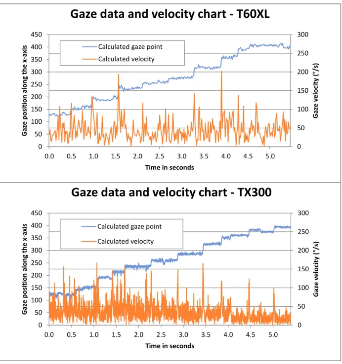
Calculated gaze point

(6)

Figure 2. Charts showing noisy data from a a) T60XL and a b) TX300. The calculated gaze points are along the x-axis. In Figure 2, eye tracking data sampled at 60 and 300Hz can be seen plotted together with the calculated gaze velocities. The data is collected using the same test participant and the same stimuli. As can be seen in the charts, the amplitude of the noise in the velocity graphs is roughly the same while there are more peaks in the data sampled at 300Hz simply due to the higher sampling frequency, i.e. samples per time unit.

0 50 100 150 200 250 300 0 50 100 150 200 250 300 350 400 450 0.0 0.5 1.0 1.5 2.0 2.5 3.0 3.5 4.0 4.5 5.0 Gaze v e lo ci ty (° /s) Gaze p o si tion alon g t h e x -axi s Time in seconds

Gaze data and velocity chart - T60XL

Calculated velocity 0 50 100 150 200 250 300 0 50 100 150 200 250 300 350 400 450 0.0 0.5 1.0 1.5 2.0 2.5 3.0 3.5 4.0 4.5 5.0 Gaze v e lo ci ty (° /s) Gaze p o si tion alon g t h e x -axi s Time in seconds

Gaze data and velocity chart - TX300

(7)

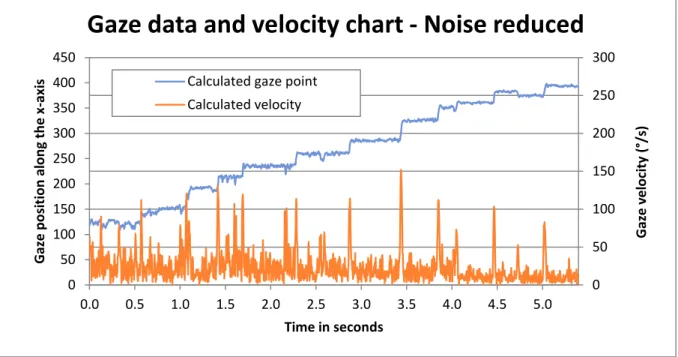
Figure 3. Chart showing the same data as Figure 2b, but after a moving average noise reduction algorithm has been applied.

2.3

Low pass filters

Noise generally appears like random spikes in the data. As the noise has a higher frequency than the signal the I-VT filter aims to detect, i.e. fixations and saccades, there is a need to reduce the impact of noise by subjecting the eye tracking data to a so-called low pass filter. As illustrated in Figure 3 in comparison with Figure 2b, a low pass filter smoothes out and reduces the noise spikes by removing high frequency signals [9]. An alternative to doing low pass filtering before the I-VT classification algorithm is applied is calculating the eye movement velocity over several samples instead of just between two. This gives an average velocity over a certain time span, which is then less sensitive to noise [1].

2.4

Gap fill in

Another issue to consider when doing fixation classification with eye tracking data is that in digital measurement systems it is almost unavoidable that some data loss occurs, i.e. that a sample cannot be collected for each occasion when the measurement is done. In the context of eye tracking, data loss is often caused by the participant blinking, looking away, or that something is put between the eye tracker and the eye so the eye tracker’s view of the eyes is obscured. These kinds of data losses usually result in gaps of a hundred milliseconds or more. However, there are also occasions where data loss occurs due to other factors, e.g. delays in data transfers within the hardware systems, temporary malfunctions of hardware, time out issues, temporary reflections in prescription glasses that make it impossible for the eye tracker to identify the eyes etc [1]. In these cases, the data loss is usually much shorter than losses caused by the reasons mentioned above. If the data loss occurs in the middle of a fixation, the fixation might be interpreted by the fixation classification algorithm as two separate fixations if the lost data is not replaced by valid data. Hence, a gap fill in algorithm is needed [10].

2.5

Eye selection

In the ideal case when doing a fixation classification, it is assumed that both eyes behave identically. Therefore, only one data stream is needed for the classification algorithm. However, in reality both eyes do not always behave the same. There is often a slight difference between one eye and the other when it comes to start time and end time of fixations as well as for blinks. There can also be occasions when there are gaps in the data from one eye and not the other [8]. For that reason, a choice has to be made as to how the data from

0 50 100 150 200 250 300 0 50 100 150 200 250 300 350 400 450 0.0 0.5 1.0 1.5 2.0 2.5 3.0 3.5 4.0 4.5 5.0 Gaze v e lo ci ty (° /s) Gaze p o si tion alon g t h e x -axi s Time in seconds

Gaze data and velocity chart - Noise reduced

(8)

both eyes should be converted into a single data set for the I-VT classification algorithm to use when classifying the samples included in the data.

2.6

Check for fixations located close in time and close in space

A weakness with the I-VT classification algorithm is that it assumes perfect data. Even with a low pass filter and gap “fill-in” algorithms, some imperfections such as short gaps or noise are preserved and result in some data points being classified incorrectly. In most cases this means that what should have been a long fixation gets classified as two shorter ones with a saccade with a very short duration and with a short offset in terms of visual angle between them. This means that after the I-VT filter has been run and the classification has been made, the resulting data needs to be post-processed for identification and merging of fixations that are very close in time and very close in space [1].

2.7

Check for short fixations

Another issue with the I-VT algorithm is that it only checks for each data point whether it is recorded while the gaze shift had a velocity that exceeded a specified threshold and, if so, labels it as being a fixation. If it is not labeled as a part of a fixation, it is assumed to be either a gap or a saccade. There is nothing within the basic classification algorithm that limits how short a fixation can be [2]. Since various cognitive and other processes, as well as visual input collection, takes place during fixations, a fixation (which is when this visual input is collected) cannot be infinitely short [11]. Therefore, a filter is needed to remove data points or groups of data points that are labeled as fixations by the I-VT filter but last too short a time for the visual input to be registered by the brain [12].

3

The Tobii Studio implementation of the Tobii I-VT filter

In the previous section, the general reasoning behind why the different functions are needed was presented. In this section we will go through how the Tobii I-VT filter, including its different parts, is implemented and why.

(9)

3.1

How it is implemented

As described above, only using the I-VT classification algorithm on unprocessed eye tracking data can result in unwanted misclassification of sample points. Therefore, in Tobii Studio there is the option to apply all the additional data processing functions that have previously been discussed. The functions are applied sequentially and individually for each recording. Consequently, if a function is applied, or a parameter for a function is modified, it influences the data used in all the following functions. It is also important to remember that all recordings in a study are subjected to the same filtering, i.e. it is not possible to adjust the parameters of the different functions in the Tobii I-VT filter to fit each recording individually.

In the Tobii I-VT filter, there are 7 different data processing functions that can be configured. Below, each data processing function will be described in the order they are applied on the eye tracking data.

3.1.1 Gap fill-in interpolation

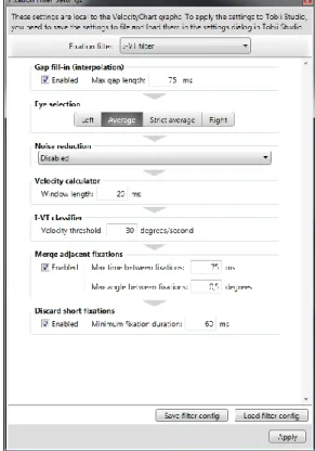
The first data processing function in the Tobii I-VT filter is the Gap fill-in interpolation. This function is not mandatory for the filter as a whole to work, but does help to fill in data where data is missing. Since missing data can be caused both by tracking problems as well as legitimate things like blinks or when the participant looks away from the screen, a parameter that is used to distinguish between these needs to be set if the gap fill-in interpolation is enabled. The parameter is labeled ‘Max gap length:’ and limits the maximum length of a gap that should be filled-in, i.e. the maximum duration a gap can be without being treated as a ‘legitimate’ gap such as a blink or data loss caused by the participant looking away or obscuring the eye tracker. The gap fill-in interpolation implementation iterates through the entire set of collected samples and each sample is subjected to the same procedure. The gap fill-in function is performed for the data collected from each eye separately. In the following paragraphs, the implementation of the gap fill-in function and the different steps involved is explained.

3.1.1.1 Identifying gaps to fill in

The first thing that happens is that the sample is tested to see whether it contains valid gaze data or not. This is done by checking the validity codes in the sample. The validity code is given per eye and is 0 if the eye is found and the tracking quality good. If the eye cannot be found by the eye tracker the validity code will be 4. The codes between 0 and 4 signify the certainty with which the eye tracker has detected the eye the validity code is associated with. If the data is deemed trustworthy, i.e. with a validity code of 0 or 1, the algorithm checks if the previous samples contained valid data as well. If they did not and the time difference in the time stamps from the last sample with valid gaze data and the current sample is less than the set ‘Max gap length’, the invalid data in the samples before the current sample is replaced by valid data.

3.1.1.2 Separating gaps that should be kept from gaps that should be filled in

If the current sample does not contain valid gaze data, the next thing that happens is that a counter, which keeps track of how many invalid samples have been detected since the last valid sample, is checked against the ‘Max gap length’ parameter. If the number of samples, including the current sample, exceeds the ‘Max gap length’ parameter, the gap is registered as a ‘valid’ gap and kept. Valid gaps are gaps that are presumed to be caused by events like blinks, temporal obstruction of the eye tracker’s view of the eyes, or the participant turning away from the eye tracker. If the current gap duration is less than the ‘Max gap length’ the counter is increased by adding the current, invalid sample.

Once one of the procedures above has been performed for the current sample, the next sample is collected and the procedure is repeated for that sample as well as for all the following samples in the recording.

3.1.1.3 Interpolating the missing data

The data in each sample in the gap, i.e. each sample before the valid sample, is replaced individually. This is done in three steps: First, a scaling factor is created. The scaling factor is created by dividing the timestamp of the sample that is going to be replaced minus the timestamp of the last valid sample before the gap by the

(10)

total duration of the gap (see Equation 1). Secondly, the scaling factor is multiplied with the position data of the first valid sample after the gap. Thirdly, the result is added to the position data of the last valid sample before the gap.

Equation 1. Calculating the scaling factor.

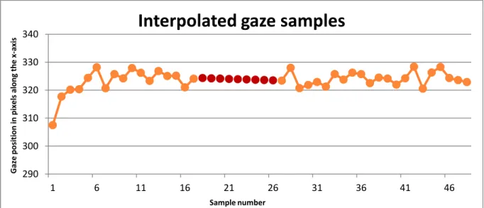
This creates a straight line of now valid and replaced samples in the data from the last valid sample before the gap to the first valid sample after the gap (see Figure 5). As can be seen by the example illustrated in Figure 5, this interpolation introduces an artificial and ideal set of data points, which are not suitable for analysis when studying details of eye movements such as saccade trajectories or microsaccades.

Figure 5. Missing or invalid samples have been replaced by interpolated samples. The interpolated samples are highlighted in red.

3.1.1.4 Setting the ‘Max gap length’ parameter

An important aspect to consider when setting the ‘Max gap length’ is that it should not fill in blinks and other gaps caused by the participant or researcher, e.g. the participant turning away from the eye tracker or the eye tracker’s view of the participant’s eyes being obstructed. Therefore, the value chosen should be shorter than a normal blink. A value used by, e.g., Komogortsev et. al. [3] is 75ms and this is also the value chosen by Tobii as the default value for this parameter. This value also corresponds well with values reported in other eye tracking studies [13], [14].

Another aspect of the gap fill-in interpolation is that it might prolong or shorten the duration of fixations and saccades. This is due to the linear interpolation and means that the measured speed between two samples within the gap will be identical and, if that velocity is below the ‘Velocity threshold’ parameter in the I-VT classification filter, all samples within the gap will then be classified as fixation samples. Whether the samples in a gap will be classified as saccade or fixation samples depends on the position data of the last valid sample before the gap and the first valid sample after the gap. If they are located close together, the samples will be classified as fixation samples. Otherwise the samples will be classified as saccade samples.

The gap fill-in interpolation function is useful for replacing a few missing samples, but is not necessary unless recordings are missing a considerable amount of data. The default setting for this function is that it is enabled. This is because the function is deemed to provide more benefits than drawbacks in the general case and make the eye tracking data analysis less sensitive to unforeseen disturbances that cause short gaps in the data during in the data collection.

290 300 310 320 330 340 1 6 11 16 21 26 31 36 41 46 G az e pos it ion in pi xe ls al ong t he x -axi s Sample number

(11)

3.1.2 Eye selection

The Tobii I-VT filter implementation has four options for selecting how to merge the data collected from two eyes into one data set that is then going to be used in the steps that follow within the Tobii I-VT implementation. The four options will be described in turn below:

3.1.2.1 Left or Right – Only using one eye

The right and left eye in Tobii Studio denote the eye position as seen from the eye tracker. If either the Left or the Right option is selected, only the data that is collected from the left or the right eye is used for the fixation classification. The data from one eye will only be used if the eye tracker is certain that the data collected in a sample is from the selected eye. If only one eye has been detected in a sample and the eye tracker could not with certainty determine which of the two eyes it was, the data from that sample will not be included in the following steps of the fixation classification process. However, there is one exception to this and that is if only one eye was detected during calibration. If that was the case, all samples collected during a recording will be assumed to have been collected for the eye detected during the calibration associated with the recording. If, during the calibration, only one eye was detected and two eyes are detected during the recording, only the data from the eye specified by this parameter will be used.

3.1.2.2 Average

The average option makes an average of the position data from the left and the right eye. If only one eye is detected, it uses the data from that eye even if it is not completely sure which eye has been detected. However, if only one eye is detected and the eye tracker cannot at all determine which eye it is, the data is discarded unless only one eye was detected during calibration. If only one eye was detected during the calibration and two eyes are detected during the recording, this can lead to offsets as the eye model constructed for the eye detected during the calibration will be used to calculate the gaze data for both eyes. In the general case, the left and right eyes are not identical. Therefore, using the same eye model for both will lead to inaccurate gaze estimations for the eye that the eye model was not originally constructed for.

3.1.2.3 Strict average

Unlike the ‘Average’ setting, the strict average setting discards all samples where only one eye has been detected. The data that is used is only the average created when samples from both eyes are detected. If ‘Strict average’ is selected and only data from one eye is detected, this will result in no classifications of fixations. If only one eye was detected during calibration, but two during the recording, this will lead to the same issues as described for the ‘Average’ setting.

3.1.3 Noise reduction

The Tobii I-VT filter offers the option to use a noise reduction function. A noise reduction function is useful if the collected gaze data is very noisy, but it is not mandatory for the complete Tobii I-VT filter to work. In Tobii Studio 2.4, two different noise reduction functions are available: Moving average and Median. A noise reduction function is basically a simple form of a low pass filter that aims at smoothing out the noise while still preserving the features of the sampled data needed for fixation classification [15].

3.1.3.1 Moving Average

The noise reduction algorithm implemented in the Moving Average noise reduction function is what, in signal processing terms, is known as a non-weighted moving-average filter [15] (see Equation 2). This means that the output from the signal for each sample is an average of a defined number of samples before, and a defined number of samples after, the current sample. As the previous samples and the following samples should have the same weight on the average, an equal number of previous samples and following samples should be included in the average (N in Equation 2 represents the number of previous and following samples). The current sample is also included in the average. This means that the total number of included samples in such an averaging window (including the current sample) needs to be an odd number (2*N+1 in Equation 2). The averaging window size can be set in the ‘Window size’ parameter.

(12)

Equation 2. Non-weighted moving average filter equation.

As the averaging window uses both data from before and after the current sample, situations regularly occur when such data is not available, i.e., in the beginning of a recording, before and after a gap as well as at the end of a recording. The way that the noise reduction algorithm is implemented then adjusts the window size to only include samples with valid gaze data while still remaining symmetrical. This means that the average close to the beginning and end of a recording or before and after a gap will be calculated using fewer samples than elsewhere. As a result, the calculated value might contain more influence from noise than where the calculations have been made using more samples. In the extreme cases of the last sample before a gap and the first sample after a gap this means that no noise reduction has been performed at all.

Any kind of filter has both wanted and unwanted consequences on the resulting data. Whether a filter should be used or not should only be determined after evaluating the benefits and drawbacks involved with that specific filter in the specific use situation. As seen above, using smaller windows has the benefit of allowing samples close to gaps to be involved in fixation classification, but also introduce the risk of these samples being incorrectly classified since the noise reduction has not been performed equally on all available samples. Also, the ‘Window size’ parameter has a lot of influence over how the samples will be classified in the I-VT classifier. The smaller the window is, the more the quick changes between the sample being classified as a saccade and a fixation will be kept, which means that the onset of a saccade or a fixation can be detected closer to the time in the recording when it actually happened. However, a smaller window also allows more of the noise to remain in the data, which means that there is a risk that false saccades and fixations will be detected.

Figure 6. Chart showing raw eye tracking data sampled at 30Hz as well as data subjected to the Moving Average noise reduction function with a window size of 3 and 5 samples.

The larger the window, the more smoothed out the data will be. This will cause the steep transitions between fixations, which can be seen in the raw data, to be transformed into smoother slopes after noise reduction has been performed (see Figure 6). As a result, the calculated velocity during the saccades will be considerably lower. Therefore, the velocity threshold needs to be adjusted accordingly. In addition, as can be seen in Figure 6, the larger the ‘Window size’ parameter, the longer the duration of the saccades and the shorter the fixations. This means that saccades will appear longer in duration and with a lower velocity, which means that short fixations preceded by lengthy saccades will become even shorter with a risk of being discarded completely if their duration is less than the value set for the ‘Discard short fixations’ parameter.

0 20 40 60 80 100 120 140 0.0 0.5 1.0 1.5 2.1 Gaze p o si tion alon g t h e x -axi s Time in seconds

Eye tracking data sampled at 30 Hz

No noise reduction Moving Average - 3 samples Moving Average - 5 samples

(13)

Figure 7. Chart showing raw eye tracking data sampled at 30 Hz as well as data subjected to the Moving Average noise reduction function with a window size of 3 samples.

Another effect the window size has on the data is that the position data in the filtered samples will be slightly altered. If the ‘Window size’ parameter in time (i.e. the number of samples multiplied by the sampling frequency’s sampling time) is not significantly shorter than the signal frequency’s period time that is to be studied, the position influence can be substantial (see the last peak of the blue and red line in Figure 6 or the orange squares compared to the red crosses in Figure 7). Due to the fact that the signal of interest and the one that should be kept unchanged mostly consists of artifacts created by fixations, it might be worth keeping in mind that the eye moves an average of two to five times per second, i.e. it makes two to five fixations per second [16]. Viewing eye movements as a signal, this would mean that the typical signal frequency would be somewhere between 2 and 5 Hz. This corresponds to a signal period time (i.e. typical fixation duration) between 200 and 500 ms since the period time is calculated by dividing 1 second by the signal frequency. If a noise reduction algorithm with a window size parameter set to 3 samples was applied to data sampled by 30 Hz it would mean that the window size would in reality be 3 times 1 second divided by 30, which equals 100ms. Since 100ms is not significantly shorter than typical fixation duration of 200ms, it indicates that applying noise reduction with this parameter setting on data sampled with this sampling frequency risks influencing the data negatively.

Figure 8. Chart showing raw eye tracking data sampled at 30 Hz as well as data subjected to the Median noise reduction function with a window size of 3 samples.

3.1.3.2 Median

A median noise reduction algorithm iterates a sliding window through the data stream much like the Moving Average algorithm. However, the middle data point is replaced with coordinates that are median values for the set of points in the window. In the Tobii Studio implementation of the median noise reduction function, the

120 130 140 150 160 50 70 90 110 130 150 170 190 210 Gaze p o si tion alon g t h e y -axi s

Gaze position along the x-axis

Raw and noise reduced data

Moving Average 3 samples No noise reduction 120 130 140 150 160 50 70 90 110 130 150 170 190 210 GAze p o si tion alon g th e y -axi s

Gaze position along the x-axis

Raw and noise reduced data

Median 3 samples No noise reduction

(14)

new x- and y- screen coordinates are calculated independently. In this example for a window containing 3 data points, [12, 5], [10, 30] and [15, 20], the middle point [10, 30] will be replaced by a new data point, [12, 20]. Here, 12 is the median of the x coordinates (10, 12, 15) and 20 is the median of the y coordinates (5, 20, 30). The benefit of a median noise reduction algorithm compared to a moving average algorithm is that the data it produces is less smoothed even though the most prominent noise is removed (see Figure 9). In addition, less ‘false’ gaze coordinates are created (see Figure 7 and Figure 8). Another benefit is that the amplitude of the velocity peaks is not reduced as severely when using the Median algorithm compared to when using the Moving average noise reduction algorithm.

Figure 9. Chart showing raw eye tracking data sampled at 30Hz as well as data subjected to the Moving Average noise reduction function and the Median noise reduction filter. Both filters were set to use a window of 5 samples.

The I-VT classification algorithm is, as discussed in the Noise section, equally sensitive to noise in eye tracking data sampled with a higher frequency as data sampled with a lower frequency. However, taking into account the drawbacks of applying the noise reduction function to data sampled with a low frequency eye tracker (60Hz or lower), extreme care should be taken when using such an algorithm for these.

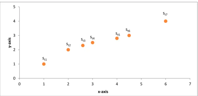
Figure 10. Illustration of consecutive gaze samples in a two dimensional coordinate system.

3.1.4 Velocity calculator

Before the I-VT classification algorithm can classify samples as belonging to a fixation or not, the samples need to be associated with a velocity. The simplest way of doing this would be to calculate the distance between the

80 100 120 140 160 180 200 220 0.0 0.5 1.0 1.5 Gaze p o si tion alon g t h e x -axi s Time in seconds

Eye tracking data sampled at 30 Hz

No filter Moving Average - 5 samples Median - 5 samples 0 1 2 3 4 5 0 1 2 3 4 5 6 7 y-axi s x-axis

s

t1

s

t2

s

t3

s

t5

s

_t4

s

t6

s

t7

(15)

gaze data points (e.g. st1 and st2 in Figure 10) in two consecutive samples and divide it by the sampling time or time between two samples (see Equation 3).

Equation 3. Basic gaze velocity calculation.

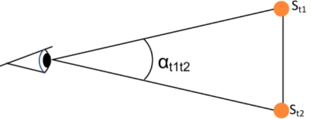
However, this would give a velocity which is related to the specific unit used to describe the size of the stimuli which would mean that the velocity threshold would need to be recalculated whenever the relation between the unit describing the stimuli and the size of the stimuli in cm or inches as well as the distance between the study participant and the stimuli plane would change. In order to render gaze velocity independent of the image and screen resolution, the Tobii I-VT filter calculates this quantity in terms of visual angle, i.e., degrees per second. This calculation is based on the relationship between the eye position in 3D space in relation to the stimuli plane and the gaze positions on the stimuli plane. The angle is calculated by taking the eye positions for the sample the value is calculated for and using that to calculate the visual angle between the eye position and the two gaze points (see Figure 11). This is then divided by the time between the two samples to provide the angular velocity.

It is worth noting that in eye tracker firmware releases, which are built on SDK 3.0 or higher, more detailed information about where the eye is located in 3D space in relation to the eye tracker and stimuli plane is given than in previous eye tracker firmware releases. This means that the gaze velocity can be calculated with greater accuracy than with previous releases since the precise distance between the stimuli plane and the eye is accessible. The angle velocity can still be calculated with data collected with previous firmware versions, i.e. for projects created and data recorded before the release of Tobii Studio 2.3, but only the distance between the eye tracker and the eye is then known and not the 3D relation between the eye and the stimuli plane. This means that the resulting value is not as accurate as with data collected using an eye tracker with firmware based on SDK 3.0 or higher.

The complication related to calculating velocity in this way is that the higher the sampling frequency, the shorter the distance that the gaze will have time to move. Therefore, if noise then adds an additional distance of a similar magnitude as the real movement, the calculated velocity will appear to be almost twice the real velocity. This means that noise has the potential to have a substantial effect on the calculated velocities for data collected by eye trackers with a higher sampling frequency if the noise is calculated between only two consecutive samples. In order to reduce the impact of noise, the velocity calculator in the Tobii I-VT filter provides the option of calculating the angle velocity for each sample as an average of the velocity for a period of time around the current sample instead of just between two consecutive samples. The parameter ‘Window length’ is used to specify over how long a time the averaging should be done. By entering a time instead of a number of samples, it is possible to make this parameter consistent even if the sampling frequency is changed. However, in the actual velocity calculations, the window length in time is converted to a number of samples. This is done by calculating how many samples are collected within the time span given in the ‘Window length’ parameter. As the time between samples can vary during a recording, even if it is only by a millisecond or so

St1

St2

α

t1t2

(16)

[17], the number of samples in an interval is calculated by first making a calculation of the average differences in timestamps between the first 100 samples in a recording and then dividing the ‘Window length’ parameter with the resulting value. The number given by this calculation is then added by one as there will always be one sample at the beginning of an interval, i.e. at time zero (t=0). This implementation of the ‘Velocity calculator’ also safeguards against only one sample being within the given parameter duration by setting the minimum number of used samples in a velocity calculation to two. This is because at least two samples are needed to make any such calculation at all.

The average velocity for a sample is calculated by creating a window in which that sample is the middle sample. To calculate the velocity, three pieces of information regarding position is needed. These are the gaze point position data on the stimuli for the first and last samples in the window and the eye position data from the middle sample, i.e. the sample the velocity is calculated for. By knowing the eye position data from the sample for which the velocity is to be calculated, it is possible to determine the visual angle between the stimuli gaze point from the first sample and the point from the last sample in the window (see Figure 11). Once this angle is determined, the difference in timestamps from the first and last sample is used to find out the time between these samples. By dividing the visual angle between the points in relation to the eye position by the time difference, the gaze velocity is determined. This is then repeated for all samples in the data. In order to ensure that the velocity is calculated in the same way for all samples, no calculation is made if there are not enough samples available to fill the window. This means that there will be no velocity calculated for samples within half a ‘Window length’ duration from a gap or beginning or end of a recording.

When setting the ‘Window length’ parameter it is important to evaluate the consequences of the selected value. Because the ‘Velocity calculator’ has properties similar to a low pass filter, a high value set as the ‘Window length’ parameter will smooth out rapid changes in the velocity. Therefore, the I-VT classification algorithm will be less sensitive to quick onsets of saccades or fixations. In addition, as no calculations of velocity will be made before or after gaps for half the duration of the ‘Window length’ parameter, a high value will make the duration of gaps in the data increase. However, a too low value will, if the data is noisy, create a risk that samples will be wrongly classified since the influence from the noise will be higher.

The default value for the ‘Window length’ parameter is 20ms. This value has been found to handle a reasonable level of noise without distorting the data too much as well as providing consistent results independent of sampling frequency.

3.1.5 I-VT classifier

The only thing an I-VT classification algorithm does is to check the velocity associated with each sample and classify the sample as either a part of a fixation or not depending on whether the velocity is below or above a set threshold. In addition, the I-VT classifier function in the Tobii I-VT filter does a few other things: Apart from classifying samples as being parts of fixations or not, it also groups consecutive samples with the same classification together in order to simplify the processing of the data in the functions that follow the I-VT classifier in the Tobii I-VT filter. It also calculates the duration and position of the fixation created after the grouping of samples with the same classification. The way the I-VT classifier is implemented in the Tobii I-VT filter corresponds to the process described by Komogortsev et al. [3] and is described below.

For each sample, the velocity is checked and the sample is classified as either a fixation or saccade: If the velocity associated with a sample is below the ‘Velocity threshold’ parameter, that sample is classified as belonging to a fixation and if it is the same or higher than the parameter, it is classified as belonging to a saccade. The exception is for samples where the velocity is not included, e.g. for samples within gaps or in the beginning or end of a recording where it has not been possible to calculate the velocity.

(17)

0 50 100 150 200 250 300 0 50 100 150 200 250 300 350 400 450 0.0 0.5 1.0 1.5 2.0 2.5 3.0 3.5 4.0 4.5 5.0 G az e v e loci ty ( °/s) G az e pos it ion al ong t he x -axi s Time in seconds

Gaze data and velocity chart - low

noise level

Calculated gaze point Calculated velocity 0 50 100 150 200 250 300 0 50 100 150 200 250 300 350 400 450 0.0 0.5 1.0 1.5 2.0 2.5 3.0 3.5 4.0 4.5 5.0 G az e v e loci ty ( °/s) G az e pos it ion al ong t he x -axi s Time in seconds

Gaze data and velocity chart - high

noise level

Calculated gaze point Calculated velocity

Once a sample has been classified, it is compared to the sample immediately preceding it. If the current and the previous sample have the same classification, the sample is added to a list that includes all consecutive samples of the same classification that have been found since the last sample with a different classification. If the current sample and the previous sample have different classifications, the list of samples with the same classification up to the current sample is used to create a fixation, saccade or gap. Calculating the duration of the fixation, saccade or gap, is done as follows: The start time is determined by taking the timestamp from the last sample in the previous list of samples with the same classification and the first sample in the current list of samples with another classification and calculating the exact point in time between these two samples. The same is done for the last sample in the current list of samples and the first sample in the list of samples after the current list. This ensures that there are no gaps between different types of eye movements in the time line, but also results in all eye movements having a duration that is one sampling time longer than the time between the first and the last sample in the list.

The position of a fixation is determined by calculating the average of the gaze position data from the samples included in a list of samples classified as belonging to a fixation. The information about the type of eye movement, the eye movement’s duration, its position information as well as all the samples belonging to this instance of the eye movement is then saved in another list containing the eye movements identified thus far up to the current sample. The current sample then becomes the first in a new list of samples with its classification. Then the next sample is collected from the data and the classification procedure is repeated for that sample.

Depending on the level of noise in the recording data, the ‘Velocity threshold’ parameter might have to be adjusted to a higher or lower value (see Figure 12). A too low value will result in more samples being wrongly classified as saccades and a too high value might increase the risk of shorter fixations being ignored. However, in some cases when the level of noise is very high, identifying a suitable velocity threshold parameter value can be very difficult (see Figure 12a).

The default value for the ‘Velocity threshold’ parameter is set to 30

°

/s [18]. The default value for the ‘Velocity threshold’ parameter was selected to be sufficient for recordings with various levels of noise. However, modifications to this setting might be necessary for recordings and projects with very noisy data.

3.1.6 Merge adjacent fixations

The grouping of samples into fixations, saccades or gaps is done without considering how many samples are included in each group. This means that if one or a small group of samples have been classified incorrectly due to being affected by noise or any other disturbance that might cause such a thing, this can cause a long fixation to be divided into several short ones with very short saccades or gaps in between. If fixations are located close Figure 12. Charts showing the calculated gaze and gaze velocity as well as a line representing a velocity threshold parameter of 30

°

/s.

(18)

together both in time and space, it is very likely that they actually are parts of one long fixation and that measurement errors have caused the fixation to be split up. The ‘Merge adjacent fixations’ function can be used to stitch together parts of a fixation that have been split up [3]. By specifying the maximum time between two fixation parts (the ‘Max time between fixations’ parameter) before they should be seen as separate fixations as well as the maximum visual angle between the fixations parts (the ‘Max angle between fixations’ parameter), it is possible to define how this merging should be done.

To test if two consecutive fixations should be merged, the first thing that is verified is if the time between the end of the first fixation and the beginning of the next is shorter than the time specified in the ‘Max time between fixations’ parameter. If so, the visual angle between the positions of the two fixations is determined. This is done by calculating an average eye position from the eye position data from the last sample in the first fixation and the first sample from the next fixation and, by using that eye position, determining the visual angle between the fixation position of the first fixation and the next fixation. If that angle is smaller or equal to the angle set in the ‘Max angle between fixations’ parameter the two fixations are merged.

When selecting the ‘Max time between fixations’ parameter it is important to set a value that does not remove blinks, i.e. it needs to be lower than a blink duration. Otherwise, the resulting data might be misleading. The default value for the ‘Max time between fixations’ parameter is selected to be lower than what is commonly reported as normal blink durations for short blinks [3], [14], [19]. The default value is 75 ms and is the same value as used by Komogortsev et al. [3] for this purpose.

In addition, selecting a too large value for the ‘Max angle between fixations’ parameter might result in merging of fixations that should have been separated by a short saccade. Regarding the ‘Max angle between fixations’ parameter, this value is selected based on a literature review of studies where this algorithm is used to merge fixations. The selected default value of 0.5° is an average of what is commonly used [3], [20–22] and also corresponds well with allowing short microsaccades and other minor eye movements to take place during fixations without splitting them up [12].

3.1.7 Discard short fixations

Even if the ‘Merge adjacent fixations’ function has been used, there might still be fixations with very short durations remaining. A very short fixation is not meaningful when studying user behavior since the eye and brain require some time for the information of what is seen to be registered [1]. Therefore, the ‘Discard short fixations’ function provides the option to remove fixations that are shorter than a set value from the list of fixations. This value is set by the ‘Minimum fixation duration’ parameter. The way this is implemented in the Tobii I-VT filter is that the duration of each fixation is checked against the ‘Minimum fixation duration’ parameter individually. If the duration is shorter than the parameter value, the fixation is reclassified as an unknown eye movement.

The default value for the ‘Minimum fixation duration’ parameter is selected to allow for fairly short fixations (60ms) as these are commonly available during reading [3], [12], [20], [23] and a substantial amount of eye tracking research includes analysis of eye movements during reading.

3.2

The Tobii I-VT filter and Tobii Glasses

The Tobii I-VT filter is developed to work for stationary eye trackers. Therefore, Tobii does not currently provide any recommendations regarding settings if choosing to use this filter for data collected using Tobii Glasses. Because the glasses, even when a snapshot is used, do not provide a very specific distance between the stimuli plane, i.e. the snapshot plane and the eye, all calculations in the filter that involve gaze points and eye positions are prone to introduce fixation data that is more or less incorrect. The settings for merging fixations can be particularly tricky to set since this requires the distance between the eye and the stimuli to be known. In addition, with the relatively low sampling frequency of the Tobii Glasses, the data should not be

(19)

subjected to low pass filtering as this might remove important information in the data that is needed for samples to be classified correctly as saccades, fixations or gaps.

3.3

Selecting settings

Depending on noise levels as well as which stimulus is used, the values for the different parameters in the Tobii I-VT filter might have to be modified. The default values are selected to provide consistent results for eye trackers with different sampling frequencies and recordings with different levels of noise. However, as always when trying to identify values that should work for a variety of situations, the selected values are not optimized for any particular kind of study or level of noise. For studies where the noise level is low, e.g., the velocity threshold can be set lower, and in studies where the stimuli is constructed so most saccades stretch over long distances, the velocity threshold can be set higher without losing any fixation information. By inspecting the data using the ‘Gaze velocity’ tool in Tobii Studio it is possible to form an idea of whether the current settings are sufficient of if they should be modified.

(20)

4

Bibliography

[1] S. M. Munn, L. Stefano, and J. B. Pelz, “Fixation-identification in dynamic scenes,” in Proceedings of the 5th symposium on Applied perception in graphics and visualization - APGV ’08, Los Angeles, California, 2008, p. 33.

[2] D. D. Salvucci and J. H. Goldberg, “Identifying fixations and saccades in eye-tracking protocols,” in Proceedings of the symposium on Eye tracking research & applications - ETRA ’00, Palm Beach Gardens, Florida, United States, 2000, pp. 71-78.

[3] Komogortsev, Oleg V., Gobert, Denise, V., Jayarathna, Sampath, Koh, Do Hyong, and Gowda, Sandeep M., “Standardization of Automated Analyses of Oculomotor Fixation and Saccadic Behaviors,” Biomedical Engineering, IEEE Transactions on, vol. 57, no. 11, pp. 2635 - 2645.

[4] R. Lans, M. Wedel, and R. Pieters, “Defining eye-fixation sequences across individuals and tasks: the Binocular-Individual Threshold (BIT) algorithm,” Behav Res, Nov. 2010.

[5] K. Rayner, “Eye movements in reading and information processing: 20 years of research.,” Psychological Bulletin, vol. 124, no. 3, pp. 372-422, 1998.

[6] J. Chen, Y. Tong, W. Gray, and Q. Ji, “A robust 3D eye gaze tracking system using noise reduction,” in Proceedings of the 2008 symposium on Eye tracking research & applications - ETRA ’08, Savannah, Georgia, 2008, p. 189.

[7] J. Klingner, R. Kumar, and P. Hanrahan, “Measuring the task-evoked pupillary response with a remote eye tracker,” in Proceedings of the 2008 symposium on Eye tracking research & applications - ETRA ’08, Savannah, Georgia, 2008, p. 69.

[8] A. Duchowski, Eye tracking methodology : theory and practice, 2nd ed. London: Springer, 2007. [9] J. Doyne Farmer, “Optimal shadowing and noise reduction,” Physica D: Nonlinear Phenomena, vol. 47, no. 3, pp. 373-392, Jan. 1991.

[10] O. V. Komogortsev, D. V. Gobert, and Z. Dai, “Classification Algorithm for Saccadic Oculomotor Behavior,” Dept. of Computer Science, Texas State University-San Marcos, Technical Report TXSTATE-CS-TR-2010-23, 5 2010.

[11] J. M. Henderson and T. J. Smith, “How are eye fixation durations controlled during scene viewing? Further evidence from a scene onset delay paradigm,” Visual Cognition, vol. 17, no. 6–7, pp. 1055-1082, Aug. 2009.

[12] J. Salojärvi, K. Puolamäki, J. Simola, L. Kovanen, I. Kojo, and S. Kaski, “Inferring relevance from eye movements: Feature extraction,” in Helsinki University of Technology, 2005, p. 2005.

[13] S. Benedetto, M. Pedrotti, L. Minin, T. Baccino, A. Re, and R. Montanari, “Driver workload and eye blink duration,” Transportation Research Part F: Traffic Psychology and Behaviour, vol. 14, no. 3, pp. 199-208, May 2011.

[14] M. Ingre, T. Akerstedt, B. Peters, A. Anund, and G. Kecklund, “Subjective sleepiness, simulated driving performance and blink duration: examining individual differences,” J Sleep Res, vol. 15, no. 1, pp. 47-53, Mar. 2006.

(21)

[16] T. A. Salthouse and C. L. Ellis, “Determinants of Eye-Fixation Duration,” The American Journal of Psychology, vol. 93, no. 2, p. 207, Jun. 1980.

[17] Tobii Technology AB, “Timing Guide for Tobii Eye Trackers and Eye Tracking Software.” Tobii Technology AB, 23-Feb-2010.

[18] A. Olsen and R. Matos, “Identifying parameter values for an I-VT fixation filter suitable for handling data sampled with various sampling frequencies,” in ETRA ’12, Santa Barbara, CA, USA.

[19] F. Volkmann, L. Riggs, and R. Moore, “Eyeblinks and visual suppression,” Science, vol. 207, no. 4433, pp. 900-902, Feb. 1980.

[20] E. A. B. Over, I. T. C. Hooge, B. N. S. Vlaskamp, and C. J. Erkelens, “Coarse-to-fine eye movement strategy in visual search,” Vision Research, vol. 47, no. 17, pp. 2272-2280, Aug. 2007.

[21] C. Nakatani and C. van Leeuwen, “A pragmatic approach to multi-modality and non-normality in fixation duration studies of cognitive processes,” Journal of Eye Movement Research, vol. 1, no. 2, pp. 1-12, 2008.

[22] R. Kliegl, E. Grabner, M. Rolfs, and R. Engbert, “Length, frequency, and predictability effects of words on eye movements in reading,” European J. of Cognitive Psych., vol. 16, no. 1, pp. 262-284, 2004.

[23] R. Radach, L. Huestegge, and R. Reilly, “The role of global top-down factors in local eye-movement control in reading,” Psychological Research, vol. 72, no. 6, pp. 675-688, Oct. 2008.