Financial Incentives in Health Care Reform: Evaluating Payment
Reform in Accountable Care Organizations and Competitive
Bidding in Medicare
(Article begins on next page)
The Harvard community has made this article openly available.
Please share
how this access benefits you. Your story matters.
Citation
Song, Zirui. 2012. Financial Incentives in Health Care Reform:
Evaluating Payment Reform in Accountable Care Organizations
and Competitive Bidding in Medicare. Doctoral dissertation,
Harvard University.
Accessed
April 17, 2018 3:38:30 PM EDTCitable Link
http://nrs.harvard.edu/urn-3:HUL.InstRepos:10344923
Terms of Use
This article was downloaded from Harvard University's DASH
repository, and is made available under the terms and conditions
applicable to Other Posted Material, as set forth at
http://nrs.harvard.edu/urn-3:HUL.InstRepos:dash.current.terms-of-use#LAA
© 2012 – Zirui Song
All rights reserved.
iii
Dissertation Advisor: Michael E. Chernew, Ph.D. Zirui Song
Financial Incentives in Health Care Reform: Evaluating Payment Reform in Accountable Care Organizations and Competitive Bidding in Medicare
Abstract
Amidst mounting federal debt, slowing the growth of health care spending is one of the nation’s top domestic priorities. This dissertation evaluates three current policy ideas: (1) global payment within an accountable care contracting model, (2) physician fee cuts, and (3) expanding the role of competitive bidding in Medicare.
Chapter one studies the effect of global payment and pay-for-performance on health care spending and quality in accountable care organizations. I evaluate the Blue Cross Blue Shield of Massachusetts Alternative Quality Contract (AQC), which was implemented in 2009 with seven provider organizations comprising 380,000 enrollees. Using claims and quality data in a quasi-experimental difference-in-differences design, I find that the AQC was associated with a 1.9 percent reduction in medical spending and modest improvements in quality of chronic care management and pediatric care in year one.
Chapter two studies Medicare’s elimination of payments for consultations in the 2010 Medicare Physician Fee Schedule. This targeted fee cut (largely to specialists) was accompanied by a fee increase for office visits (billed more often by primary care physicians). Using claims data for 2.2 million Medicare beneficiaries, I test for
discontinuities in spending, volume, and coding of outpatient physician encounters with an interrupted time series design. I find that spending on physician encounters increased 6
iv
percent after the policy, largely due to a coding effect and higher office visit fees. Slightly more than half of the increase was accounted for by primary care physician visits, with the rest by specialist visits.
Chapter three examines competitive bidding, which is at the center of several proposals to reform Medicare into a premium support program. In competitive bidding, private plans submit prices (bids) they are willing to accept to insure a Medicare beneficiary. In perfect competition, plans bid costs and thus bids are insensitive to the benchmark. Under imperfect competition, bids may move with the benchmark. I study the effect of benchmark changes on plan bids using Medicare Advantage data in a
longitudinal market-level model. I find that a $1 increase in the benchmark leads to about a $0.50 increase in bids among Medicare managed care plans.
v
Table of Contents
Abstract ... iii
Acknowledgements ... vii
Chapter 1. Effect of the Blue Cross Blue Shield of Massachusetts Alternative Quality Contract on health care spending and quality 1.1 Introduction ...2 1.2 Methods...4 1.2.1 Population ...4 1.2.2 Study design ...4 1.2.3 Empirical approach ...7 1.3 Results ...8 1.3.1 Spending ...8 1.3.2 Quality...13 1.3.3 BCBS payments ...15 1.4 Discussion ...15 1.5 References ...18 1.6 Supporting Materials ...22
Chapter 2. Unintended consequences of redistributing Medicare payments from specialists to primary care physicians 2.1 Introduction ...34 2.2 Methods...36 2.2.1 Population ...36 2.2.2 Study design ...36 2.2.3 Empirical approach ...37 2.3 Results ...40 2.3.1 Spending ...41 2.3.2 Volume ...45 2.3.3 Complexity ...45 2.4 Discussion ...48 2.5. References ...52 2.6 Supporting Materials ...55
vi
Chapter 3. Competitive bidding in Medicare Advantage: Effect of benchmark changes on plan bids
3.1 Introduction ...61
3.2 Background ...64
3.2.1 Competitive bidding in Medicare Advantage ...66
3.3 Theory ...69
3.3.1 Perfect competition (Bertrand pricing) ...69
3.3.2 Imperfect competition (Nash pricing) ...70
3.4 Data ...72 3.5 Empirical strategy ...73 3.5.1 Level of analysis ...73 3.5.2 Empirical model ...74 3.5.3 Potential endogeneity ...76 3.5.4 Instrumental variables ...78 3.6 Results ...79 3.6.1 Descriptive analyses...79 3.6.2 Econometric results ...81
3.6.3 Sensitivity analyses related to endogeneity ...86
3.6.4 Effect on rebates ...88
3.7 Conclusion ...88
3.8 References ...91
vii
Acknowledgements
This dissertation was made possible by the incredible support and guidance of the faculty members on my dissertation committee. They have inspired me, challenged me, and created a most rewarding and enjoyable experience in the Ph.D. program.
I am foremost indebted to Professor Michael Chernew for giving me the
opportunity to embark on this series of research projects, for his daily collaboration and feedback, and for his broader mentorship. I am incredibly grateful to Professor John Ayanian for many discussions of research ideas during my early years in the program, for his clinical expertise, and for serving as a physician role model to me. I deeply appreciate Professor Thomas McGuire in numerous ways, from helping me think through countless research ideas in their nascent stages, to always giving his time to debrief after a research talk, and to playing basketball and other fun times outside of the office. I am eternally grateful to Professor Joseph Newhouse for admitting me into the program, for serving as the faculty advisor to my student fellowship from the National Institute on Aging, and for always giving his time and thought to my work.
I have also benefited from the advice, mentorship, and collaboration of other faculty members in the Ph.D. program and broader health policy community, including Professors Katherine Baicker, Amitabh Chandra, David Cutler, Randy Ellis, John Hsu, Haiden Huskamp, Bruce Landon, Frank Levy, Barbara McNeil, Michael McWilliams, Dana Safran, and Jonathan Skinner. My dissertation work took place at the Department of Health Care Policy, where I was the beneficiary of help from many staff members and administrators, including Emily Corcoran, Debby Collins, Wilma Stahura, and the team at the HCP Help Desk.
viii
I thank my fellow classmates in the Ph.D. program, who have provided an amazing community of friends and colleagues. I especially appreciate everyone in the entering cohort of 2008, whose friendship and support have helped make these years meaningful and memorable. They are Mike Botta, Rebecca Cadigan, Laura Garabedian, Keren Ladin, Nick Menzies, Jessica Perkins, Tisamarie Sherry, Sae Takada, Melissa Valentine, and Beth Wikler. Classmates from adjacent cohorts in the Economics track of the Ph.D. program have also provided a wonderful community for exchanging ideas and feedback. I would like to especially acknowledge Martin Andersen, Sebastian Bauhoff, Abby Friedman, Daria Pelech, Sam Richardson, Aaron Schwartz, Tisamarie Sherry, and Jacob Wallace. Our Health Policy program office has always provided tremendous support and been the backbone of the program in many ways. Special thanks goes to Debbie Whitney, Ayres Heller, Kristin Collins, and Joan Curhan.
Generous funding for graduate school and parts of medical school was provided by a National Institute on Aging Predoctoral M.D./Ph.D. National Research Service Award (F30 AG039175), a Pre-doctoral Fellowship in Aging and Health Economics from the National Bureau of Economic Research (T32 AG000186), and a training grant from the Agency for Healthcare Research and Quality to our Health Policy program.
My deepest gratitude goes to my parents, for teaching me the most important lessons in life and never wavering from their unconditional love and support. They have sacrificed so much over so many years for me. I dedicate this dissertation to them. Finally, I am also indebted to my most supportive friend and partner in life in recent years, Katherine Koh, whose undying faith in me and steadfast encouragement have blessed me with a source of strength that always restores me.
1
Chapter 1
Effect of the Blue Cross Blue Shield of Massachusetts Alternative
Quality Contract on health care spending and quality*
* A version of this chapter was previously published as the following:
Zirui Song, Dana G. Safran, Bruce E. Landon, Yulei He, Randall P. Ellis, Robert E. Mechanic, Matthew P. Day, and Michael E. Chernew, “Health Care Spending and Quality in Year 1 of the Alternative Quality Contract,” New England Journal of Medicine. 2011 Sept 8;365(10):909-18. Epub 2011 July 13.
2
1.1. Introduction
The growth of health care spending is a major concern for households, businesses, and state and federal policymakers.1-3 In response to continued spending growth in
Massachusetts following health care reform, Blue Cross Blue Shield of Massachusetts (BCBS), the state’s largest commercial payer, implemented the Alternative Quality Contract (AQC) in January of 2009.4 The AQC is a contracting model based on global payment and pay-for-performance. It is similar to the two-sided accountable care
organization (ACO) model specified by the Centers for Medicare and Medicaid Services (CMS) in its proposed ACO regulations.5
Global payment has received attention as an alternate financing mechanism to fee-for-service (FFS) because of its ability to control total spending.6-7 In July of 2009, a Massachusetts state commission voted unanimously to move the state towards global payment within 5 years.8 In contrast to a one-sided, “shared savings” model in which providers do not bear risk, providers in a global payment model share in savings if
spending is below a pre-specified budget, but are also accountable for deficits if spending exceeds the budget. 9-11 This “downside” risk is a stronger tool for spending control.12-14
BCBS implemented the AQC in its health maintenance organization (HMO) and point-of-service (POS) enrollee population. These plans require enrollees to designate a primary care physician (PCP), a feature also found in many patient-centered medical home models.15-19 Presently, the AQC does not extend to PPO enrollees, as they are not required to designate a PCP. Thus, when a provider organization enters the AQC, only its HMO/POS patients are encompassed by the contract.
3
The AQC contains 3 main features that distinguish it from traditional fee-for-service contracts and from capitation contracts locally and nationally.4 First, physicians groups, in some cases together with a hospital, enter into 5-year global budget contracts (in contrast to 1-year contracts). Baseline budgets and future budget growth are based on negotiations with BCBS, but no group was given a 2009 budget below its 2008 spending. The budget covers the entire continuum of care, including inpatient, outpatient,
rehabilitation, prescription drugs, and long-term care. The PCP’s organization is accountable for all enrollee services, regardless of whether the enrollee receives care from her PCP, the PCP’s organization, or any other provider. Since the model currently applies to only HMO/POS enrollees, enrollees must seek referrals for specialist care, consistent with those products’ benefit designs. During the year, BCBS pays claims on a FFS basis according to negotiated rates, with year-end budget reconciliation.
Second, AQC groups are eligible for pay-for-performance bonuses up to 10 percent of their budget, with ambulatory and hospital measures each comprising half of the bonus (Section 1.6.1). This potential bonus is substantially larger than typical pay-for-performance programs in the US. BCBS sets a range of pay-for-performance thresholds, or “gates,” for each measure at the beginning of the contract which remain fixed throughout the contract.4 Each measure receives an annual score based on performance. Scores are weighted and aggregated to calculate the bonus amount paid to the AQC group.
Third, AQC groups receive technical support, including spending, utilization, and quality reports from BCBS to assist them in managing their budget and improving
quality. In 2009, 7 physician organizations comprising 321 PCP practices and over 4000 total physicians began assuming risk under the AQC for over 25 percent of BCBS
4
HMO/POS enrollees. Groups ranged from large physician-hospital organizations to small independent practices united by common leadership. Some AQC groups had prior risk contracts from BCBS, while others entered from FFS contracts without financial risk. By 2011, the AQC has grown to 12 groups accounting for 44 percent of HMO/POS
enrollees. I evaluate the impact of the AQC on health care spending and ambulatory quality measures in 2009.
1.2. Methods
1.2.1 Population
The population included BCBS enrollees from January, 2006 through December, 2009. From 2,335,593 total HMO and POS members, I excluded 701,079 who were not continuously enrolled for at least one calendar year. The remaining 1,634,514 members comprised the sample for the main analyses. All AQC and non-AQC providers with BCBS patients were included.
1.2.2 Study Design
I used a pre-post, intervention-control, difference-in-difference approach to isolate the AQC effect. For the spending analyses, the pre-intervention period was 2006 through 2008 and post-intervention was 2009. The intervention group consisted of all enrollees who designated PCPs in practices that began assuming risk under the AQC in 2009. Within the intervention group, I also pre-specified 2 subgroups: one consisting of providers who had prior experience with risk-based contracts from BCBS (“prior-risk”),
5
and the other of providers who entered the AQC without BCBS risk experience (“no-prior-risk”). I hypothesized that the AQC would have a bigger effect on spending in the no-prior-risk subgroup.
I compared spending between all AQC groups and control, prior-risk groups and control, as well as no-prior-risk groups and control. For all 3 comparisons, I decomposed the AQC effect in 4 ways to understand the source of spending differences. First, I decomposed by clinical category using the Berenson-Eggers Type of Service (BETOS) classification version 2009 from CMS.20 Second, I decomposed the findings by site (inpatient versus outpatient) and type of care (professional versus facility). Third, I examined results by quartile of enrollee health risk.
Lastly, I separated the AQC effect into price and utilization components by repricing claims for each service to its median price across all providers in the study period. Repriced spending differences reflect only utilization differences. Moreover, I examined measures of utilization such as admissions or procedures directly. I further decomposed the spending differences due to price (fees) into two potential explanations: differential fee changes (AQC groups may have received lower fee increases than non-AQC) and referral pattern changes (AQC enrollees may have received more care from lower fee providers). This was done by repricing claims to the median 2009 price for each service within each practice.
The quality analysis compared performance on ambulatory process measures between all AQC groups and control using 2007-2009 data. These measures are primary care-oriented and under direct control of the AQC groups. The measures follow
6
used by most health plans. I analyzed individual measures and aggregate measures for chronic care management, adult preventive care, and pediatric care.
For the spending analysis, the dependent variable was aggregate medical spending per member per quarter (combining BCBS spending and enrollee cost sharing). I
excluded prescription drugs from the primary analysis because not all enrollees had prescription drug coverage through BCBS. Spending was computed from claims-level FFS payments made within the global budget. This is an accurate measure of medical spending based on utilization and negotiated FFS prices, but it does not capture the quality bonuses or end-of-year budget reconciliation.
For each ambulatory quality measure, the dependent variable was a dichotomous variable indicating whether the measure was met for an eligible member in a given year. Eligibility is defined by member characteristics and diagnosis; for example, diabetes measures are restricted to members with diabetes.
I controlled for age categories, interactions between age and sex, risk score, and secular trends to correct for differences in individual traits across treatment and control groups. Risk scores were calculated by BCBS from current year diagnoses, claims, and demographic information using the diagnostic-cost-group (DxCG/Verisk Health) score system,22 similar to the method used by CMS for risk adjustment of payments to
Medicare Advantage plans. Higher scores denote lower health status and higher expected spending. The DxCG score is calculated from statistical analyses using a national claims database to relate current year spending to current year diagnoses and demographic information.
7
1.2.3 Empirical Approach
All analyses were conducted at the enrollee-quarter level. I used a one-part generalized linear model with propensity weights,21 which mitigated differences in individual traits across treatment and control groups. Propensity weights were calculated using age, sex, and risk scores. For the spending analysis, the dependent variable was spending in dollars per member per quarter. The baseline model was not logarithmic-transformed because the risk score is designed to predict dollar spending. Moreover, evidence shows that linear models perform better than more complex functional forms in predicting health spending.23-26
I estimated the reduced-form model below, where Xit represents the vector of
individual characteristics (age categories, interactions between age categories and sex, and the risk score). Additional independent variables included an indicator for the intervention (aqc), indicators for each quarter (q), and quarter-intervention interactions (q*aqc). I also included an indicator for the post-intervention period (post) as well as its interaction with the intervention group (post*aqc), which produced the estimate of the policy effect. Huber-White corrections were used to adjust standard errors for clustering of multiple observations for each individual.27-28
Spendingit = αit + Xitδ + β1postt + β2aqci + β3(post*aqc)it + qtγ1 + (qt*aqci)γ2 + εit
To assess the AQC impact on quality, I estimated an analogous difference-in-difference model. For aggregate quality analysis, I pooled measures and adjusted for
8
measure-level fixed effects. Independent variables were analogous to the spending model, with year indicators in place of quarter indicators.
Qualityit = αit + Xitδ + β1postt + β2aqci + β3(post*aqc)it + yrtλ1 + (yrt*aqc)λ2 + µit
I conducted a number of sensitivity analyses (Section 1.6.3), including alterations to the statistical model, repeating analysis on subjects who were continuously enrolled throughout the 4-year study period, coding the risk score in deciles, omitting the
propensity score weights, and explicitly including enrollee cost sharing in spending. For the quality analysis, I tested robustness of the linear probability model using a logit model. I also tested for risk score changes that would be consistent with the possibility that under a global payment system, physicians may upcode to garner increased
payments, which would make AQC patients seem sicker and thus spending adjusted for health status seem lower. This was an issue in the evaluation of Medicare’s Physician Group Practice Demonstration.30 All analyses used STATA software, version 11. Results are reported with 2-tailed P values. The Harvard Medical School Office for Research Subject Protection approved the study.
1.3. Results
1.3.1. Spending
There were 380,142 subjects with at least one year of continuous enrollment from 2006 through 2009 in the intervention group and 1,351,446 such subjects in the control
9
group. Average age, sex distribution, and health risk scores were similar between the groups (Table 1.1).
Health care spending increased for both AQC and non-AQC enrollees in 2009, but the increase was smaller for AQC enrollees (Table 1.2). Statistical estimates indicated that relative to control, the AQC was associated with a $15.51 decrease in average
quarterly spending per enrollee in 2009 (p=0.007, 95 percent confidence interval -$27.21 to -$3.81), a 1.9 percent savings. In the models, the interaction of the secular trend with the AQC indicator demonstrated no significant spending trend differences between AQC and non-AQC groups prior to the intervention ($0.89, p=0.28).
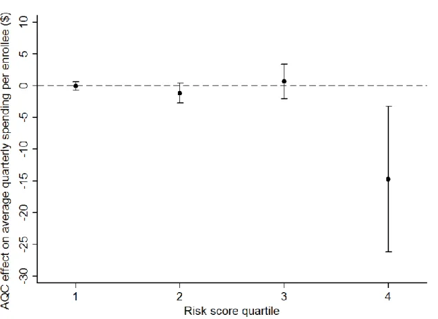
Procedures, imaging, and tests accounted for over 80 percent of the savings. Further decomposition showed that savings largely derived from spending on facility services in the outpatient setting. There were no significant changes in inpatient spending or spending on physician services. The decomposition by member health status showed that members in the highest risk quartile accounted for most (-$14.75, p=0.01) of the savings (Figure 1.1).
Models with standardized prices revealed no AQC effect on utilization. This was supported by quantity analyses of procedures, imaging, tests, admissions, and office visits. Thus, the observed savings reflect differences in price (Section 1.6.4).
Table 1.1. Characteristics of the Study Population.*
Variable All AQC Groups
(N=380,142) Control Group (N=1,351,446) Pre-AQC (2006-08) Post-AQC (2009) Pre-AQC (2006-08) Post-AQC (2009) Member characteristics Age — yr 34.4 ± 18.6 35.3 ± 18.5 35.3 ± 18.7 35.5 ± 18.8 Female sex — % 52.6 51.2 51.8 51.0
Health risk score& 1.08 (0.12—1.29) 1.16 (0.13—1.39) 1.11 (0.11—1.33) 1.16 (0.12—1.39)
* Plus-minus values are mean ± SD. Values in parentheses are the 25th and 75th percentiles. The number of total enrollees by summing treatment and control exceeds 1,634,514 because of enrollees who had a PCP in the treatment group and another in the control group for at least one year in each case.
&
Health risk score denotes enrollee health status and expected spending. It is calculated using the DxCG/Verisk Health system, which uses statistical analyses based on a national claims database to relate current year spending to current year diagnoses and demographic information. The DxCG method is a commonly used, proprietary method similar to Medicare’s Hierarchical Condition Category (HCC) system used for risk adjustment of prospective payments to Medicare Advantage plans (and developed by the same organization). DxCGs are designed for the under-65 population and are more detailed than the HCC system. Among all subjects, it ranged from 0 to 66 (mean = 1.13, standard deviation = 1.86).
1
Table 1.2. Change in average health care spending per member per quarter in AQC and non-AQC groups.*
A. All AQC groups vs. control All AQC Groups
(N=380,142)
Control Group
(N=1,351,446)
Between-Group Difference (p-value)
Pre Post Change Pre Post Change
Total quarterly spending ($) 756 808 53 785 854 69 -15.51 (0.009)
Spending by BETOS category †
1. Evaluation and management 180 206 25 181 208 27 -2.22 (0.002)
2. Procedures 166 176 10 168 184 16 -5.96 (0.001)
3. Imaging 94 102 8 100 112 11 -3.47 (<0.001)
4. Test 67 75 7 74 85 11 -3.72 (<0.001)
5. Durable medical equipment 10 12 2 11 13 2 -0.14 (0.68)
6. Other 48 50 2 54 55 1 0.80 (0.72)
7. Exceptions/Unclassified 190 189 -1 197 197 0 -0.80 (0.84)
Spending by site and type of care
Inpatient - professional 35 36 2 34 37 2 -0.72 (0.38)
Inpatient - facility 152 154 3 156 158 3 0.23 (0.95)
Outpatient - professional 316 350 34 300 334 34 -0.28 (0.80)
Outpatient - facility 214 230 16 255 285 30 -14.50 (<0.001)
Ancillary 39 39 -1 40 40 0 -0.24 (0.86)
The intervention group comprised enrollees whose primary care physicians were in the Alternative Quality Contract (AQC) system of Blue Cross Blue Shield of Massachusetts, and the control group comprised enrollees whose primary care physicians were not part of the AQC system. Blue Cross Blue Shield of Massachusetts implemented the AQC system in 2009. All
spending figures are in 2009 U.S. dollars.
† The clinical categories were designated according to the Berenson–Eggers Type of Service (BETOS) classification, version 2009.
1
12
Figure 1.1. Difference-in-difference estimates of the AQC effect on average health care spending per member per quarter, by risk quartile (all AQC groups versus control).*
* Point estimates with 95 percent confidence intervals from the baseline model.
This price effect could arise either because AQC groups received lower fee increases or because AQC enrollees were shifted to lower-fee providers. I found no differences in price trends (including hospital, non-hospital facility, and physician fees) for AQC and non-AQC providers. The model with prices standardized by physician practice revealed that the price effect was due to referral pattern changes whereby AQC patients were referred to lower-fee providers. Those providers could be in non-hospital settings (such as ambulatory surgery centers) or simply be hospitals that had lower
13
negotiated fees for outpatient care than other hospitals. This model demonstrated that referral shifts accounted for over 90 percent of the AQC-associated relative decrease in quarterly spending (-$14.21, p<0.001) in 2009 (Section 1.6.4).
The prior-risk subgroup compared to control incurred statistically insignificant total savings of $9.29 (p=0.13, -$21.45 to $2.86), or 1.1 percent, per member per quarter. In contrast, the no-prior-risk subgroup experienced larger and statistically significant savings of $45.52 (p=0.006, -$78.13 to -$12.90) or 6.3 percent, suggesting that it drove the main findings. Subgroup decompositions mirrored decompositions of main findings (Section 1.6.2). An interaction test of the differential AQC effect between the two subgroups yielded -$32.94 (p=0.06, -$66.72 to $0.83). Sensitivity analyses supported these results (Section 1.6.3).
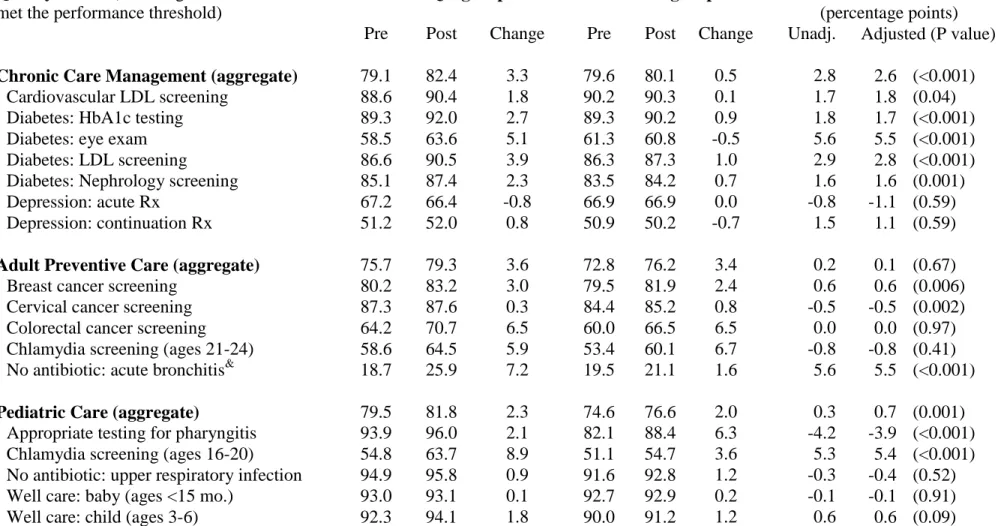
1.3.2. Quality
The AQC was associated with a 2.6 percentage-point increase in eligible members meeting quality thresholds for chronic care management (p<0.001) and a 0.7 percentage-point increase in eligible members meeting pediatric care thresholds (p=0.001) (Table 1.3). The AQC was not associated with significant improvement in adult preventive care. Comparisons between prior-risk and control as well as no-prior-risk and control yielded similar results (not shown).
Table 1.3. Change in ambulatory quality performance in AQC and non-AQC groups.*
Quality metric (% of eligible enrollees who met the performance threshold)
All AQC groups Control groups Difference
(percentage points)
Pre Post Change Pre Post Change Unadj. Adjusted (P value)
Chronic Care Management (aggregate) 79.1 82.4 3.3 79.6 80.1 0.5 2.8 2.6 (<0.001)
Cardiovascular LDL screening 88.6 90.4 1.8 90.2 90.3 0.1 1.7 1.8 (0.04)
Diabetes: HbA1c testing 89.3 92.0 2.7 89.3 90.2 0.9 1.8 1.7 (<0.001)
Diabetes: eye exam 58.5 63.6 5.1 61.3 60.8 -0.5 5.6 5.5 (<0.001)
Diabetes: LDL screening 86.6 90.5 3.9 86.3 87.3 1.0 2.9 2.8 (<0.001)
Diabetes: Nephrology screening 85.1 87.4 2.3 83.5 84.2 0.7 1.6 1.6 (0.001)
Depression: acute Rx 67.2 66.4 -0.8 66.9 66.9 0.0 -0.8 -1.1 (0.59)
Depression: continuation Rx 51.2 52.0 0.8 50.9 50.2 -0.7 1.5 1.1 (0.59)
Adult Preventive Care (aggregate) 75.7 79.3 3.6 72.8 76.2 3.4 0.2 0.1 (0.67)
Breast cancer screening 80.2 83.2 3.0 79.5 81.9 2.4 0.6 0.6 (0.006)
Cervical cancer screening 87.3 87.6 0.3 84.4 85.2 0.8 -0.5 -0.5 (0.002)
Colorectal cancer screening 64.2 70.7 6.5 60.0 66.5 6.5 0.0 0.0 (0.97)
Chlamydia screening (ages 21-24) 58.6 64.5 5.9 53.4 60.1 6.7 -0.8 -0.8 (0.41)
No antibiotic: acute bronchitis& 18.7 25.9 7.2 19.5 21.1 1.6 5.6 5.5 (<0.001)
Pediatric Care (aggregate) 79.5 81.8 2.3 74.6 76.6 2.0 0.3 0.7 (0.001)
Appropriate testing for pharyngitis 93.9 96.0 2.1 82.1 88.4 6.3 -4.2 -3.9 (<0.001)
Chlamydia screening (ages 16-20) 54.8 63.7 8.9 51.1 54.7 3.6 5.3 5.4 (<0.001)
No antibiotic: upper respiratory infection 94.9 95.8 0.9 91.6 92.8 1.2 -0.3 -0.4 (0.52)
Well care: baby (ages <15 mo.) 93.0 93.1 0.1 92.7 92.9 0.2 -0.1 -0.1 (0.91)
Well care: child (ages 3-6) 92.3 94.1 1.8 90.0 91.2 1.2 0.6 0.6 (0.09)
Well care: adolescent 73.8 76.8 3.0 69.1 71.4 2.3 0.7 0.9 (<0.001)
* Adjusted results are from a propensity-weighted difference-in-difference model controlling for all covariates and secular trends. The three aggregate analyses used pooled observations and are further adjusted for measure fixed effects.
1
15
1.3.3. BCBS Payments
The AQC-associated savings do not imply that total payments made by BCBS declined. Total BCBS payments must take into account quality bonuses and end-of-year budget surpluses paid to the AQC groups. In 2009, quality bonuses were generally between 3-6 percent of budgets. Additional BCBS support for information technology, staffing, and other needs were between 0-2 percent of budgets. Moreover, all AQC groups spent under their 2009 budget targets, earning on average 3 percent in budget surpluses (consistent with the findings). Taken together, these first year investments and payouts exceeded the average estimated savings of 1.9 percent, suggesting BCBS total payments rose for AQC groups in the first year.
1.4. Discussion
The AQC was associated with modestly lower medical spending and improved quality in the first year after implementation. The savings largely derived from shifting outpatient care to lower-fee providers, and mostly from high risk enrollees. Savings were larger among providers previously paid FFS by BCBS. These results were robust to a series of sensitivity analyses and do not appear to be attributable to upcoding. In addition, spending trends prior to the intervention were not statistically different between the AQC and non-AQC groups.
Quality improvements are likely due to a combination of substantial financial incentives and BCBS data support. AQC quality bonuses are much higher than most
pay-16
for-performance programs in the US, as it applies to the entire global budget rather than to only physician or PCP services.31
This study is subject to several limitations. The study population was young and included only POS and HMO members. Thus, results may not generalize to the Medicare population, PPO or indemnity plan enrollees, or other states. However, effects were greater for enrollees who had higher expected spending, so programs serving older populations may experience even larger savings. Furthermore, I do not observe details of each AQC contract, which varied to some degree, or details of provider risk contracting with other payers. While the results suggest quality improved, process measures do not completely capture quality. Formal evaluation of outcome measures could not be conducted due to the lack of pre-AQC enrollee-level outcomes data. However, a
weighted average of 5 outcomes metrics at the provider organization level suggests that AQC groups achieved better or comparable outcomes in 2009 compared to recent BCBS network averages (Section 1.6.5).
The findings do not imply that overall spending fell for BCBS in the first year. This reflects the design of the AQC, which focuses on slowing the growth of spending and improving quality initially rather than saving money in the first year. The AQC targets were set based on actuarial projections to save money over the 5-year contract, even after anticipated quality bonuses. Initial investments help to motivate participation and support the delivery system changes required for providers to succeed in managing spending and improving quality. Because provider groups mostly bear the risk, fiscal success from the insurer perspective depends on how well budgets and bonuses are set.
17
In total, the magnitude of savings was modest. Sustainability of the AQC and the financial viability of the model for providers will ultimately depend on identifying and addressing clinically inefficient care and changing utilization patterns. Nevertheless, the findings on referral pattern changes and quality improvements suggest that provider groups changed behavior in 2009. Importantly, referral pattern changes can subsequently affect pricing in the health care market, as high-price facilities feel pressure from
decreased volume. Future studies will need to assess whether changes in utilization and the broader market lead to larger savings.
This initial evaluation offers several lessons for payment reform.32-34 First, quality need not be threatened by global payment, and process measures can improve given clinically-aligned incentives. Other aspects of quality remain to be evaluated. Second, global payment can introduce greater price competition into the market as referrals move from high-price to low-price facilities. This is a bigger issue for private purchasers since Medicare regulates prices. Finally, even under strong financial incentives, utilization will not change rapidly. Slowing the growth rate of health care spending will ultimately depend on budget updates and the ability of providers to practice in this new environment.
18
1.5. References
1. Orszag PR, Ellis P. The Challenge of Rising Health Care Costs—A View from the Congressional Budget Office. New Engl J Med 2007;357(18):1973-5.
2. Chernew ME, Baicker K, Hsu J. The Specter of Financial Armageddon — Health Care and Federal Debt in the United States. New Engl J Med 2010;362(13):1166-8. 3. Chernew ME, Hirth RA, Cutler DM. Increased Spending On Health Care: Long-Term
Implications for the Nation. Health Aff (Millwood) 2009;28(5):1253-5.
4. Chernew ME, Mechanic RE, Landon BE, Safran DG. Private-Payer Innovation In Massachusetts: The ‘Alternative Quality Contract.’ Health Aff (Millwood)
2011;30(1):51-61.
5. Centers for Medicare and Medicaid Services. Medicare Shared Savings Program: Accountable Care Organizations. Federal Register 2011 Apr 7;76(67):19528-654. 6. Miller H. From Volume to Value: Better Ways to Pay for Health Care. Health Aff
(Millwood) 2009;28(5):1418-28.
7. Engleberg Center for Health Care Reform. Bending the Curve: Effective Steps to Address Long-Term Health Care Spending Growth. The Brookings Institution, August 2009. (http://www.brookings.edu/reports/2009/0901_btc.aspx)
8. Bebinger M. Mission Not Yet Accomplished? Massachusetts Contemplates Major Moves on Cost Containment. Health Aff (Millwood) 2009;28(5):1373-81.
9. Health Policy Brief: Accountable Care Organizations. Health Affairs, July 27, 2010. (http://www.healthaffairs.org/healthpolicybriefs/brief_pdfs/healthpolicybrief_20.pdf)
19
10.Fisher ES, Staiger DO, Bynum JP, Gottlieb DJ. Creating accountable care organizations: The extended hospital medical staff. Health Aff (Millwood) 2007;26(1):w44-57.
11.McClellan M, McKethan AN, Lewis JL, Roski J, Fisher ES. A national strategy to put accountable care into practice. Health Aff (Millwood) 2010;29(5):982-90. 12.Shortell SM, Casalino LP. Implementing qualifications criteria and technical
assistance for accountable care organizations. JAMA 2010;303(17):1747-8.
13.Devers K, Berenson R. Can Accountable Care Organizations Improve the Value of Health Care by Solving the Cost and Quality Quandaries? Urban Institute, October, 2009. (http://www.urban.org/url.cfm?ID=411975)
14.Fisher ES, Shortell SM. Accountable care organizations: accountable for what, to whom, and how. JAMA 2010;304(15):1715-6.
15.Goroll AH, Berenson RA, Schoenbaum SC. Fundamental reform of payment for adult primary care: Comprehensive payment for comprehensive care. J Gen Intern Med. 2007;22:410-5.
16.Bodenheimer T, Grumbach K, Berenson RA. A lifeline for primary care. N Engl J Med 2009;360(26):2693-6.
17.Rittenhouse DR, Shortell SM. The patient-centered medical home: will it stand the test of health reform? JAMA 2009;301:2038-40.
18.Merrell K, Berenson RA. Structuring Payment for Medical Homes. Health Aff (Millwood) 2010;29(5):852-8.
19.Kilo CM, Wasson JH. Practice Redesign and the Patient-Centered Medical Home: History, Promises, and Challenges. Health Aff (Millwood) 2010;29(5):773-8.
20
20.Centers for Medicare and Medicaid Services. Berenson-Eggers Type of Service, 2009. Available at: https://www.cms.gov/HCPCSReleaseCodeSets/20_BETOS.asp. 21.Rosenbaum PR, Rubin DB. The central role of the propensity score in observational
studies for causal effects. Biometrika 1983;70(1): 41-55.
22.Pope GC, Kautter J, Ellis RP, Ash AS, Ayanian JZ, Iezzoni LI, Ingber MJ, Levy JM, and Robst J. Risk Adjustment of Medicare Capitation Payments Using the CMS-HCC model. Health Care Financing Review 2004;25(4):119-41.
23.Zaslavsky AM, Buntin MB. Too much ado about two-part models and
transformation? Comparing methods of modeling Medicare expenditures. J Health Econ 2004;23:525-42.
24.Manning WG, Basu A, Mullahy J. Generalized modeling approaches to risk adjustment of skewed outcomes data. J Health Econ 2005;24(3):465-88.
25.Ellis RP, McGuire TG. Predictability and predictiveness in health care spending. J Health Econ 2007;26(1):25-48.
26.Ai C, Norton EC. Interaction terms in logit and probit models. Economic Letters 2003;80:123-9.
27.White H. A heteroskedasticity-consistent covariance matrix estimator and a direct test for heteroskedasticity. Econometrica 1980;48:817-30.
28.Huber PJ. The behavior of maximum likelihood estimates under non-standard conditions. In: Proceedings of the Fifth Berkeley Symposium on Mathematical Statistics and Probability. Berkeley: University of California Press, 1967:221-33. 29.Casella G, Berger RL. Statistical Inference. 2nd ed. Duxbury: Pacific Grove, 2002.
21
30.Medicare Payment Advisory Commission. Report to the Congress: Improving Incentives in the Medicare Program. 2009 June.
31.Rosenthal MB, Frank RG, Li Z, Epstein AM. Early experience with pay-for-performance: from concept to practice. JAMA. 2005 Oct 12;294(14):1788-93. 32.Shortell SM, Casalino LP, Fisher ES. How The Center For Medicare And Medicaid
Innovation Should Test Accountable Care Organizations. Health Aff (Millwood) 2010;29(7):1293-8.
33.Mechanic R, Altman S. Medicare’s Opportunity to Encourage Innovation in Health Care Delivery. N Engl J Med 2010;362(9):772-4.
34.Guterman S, Davis K, Stremikis K, Drake H. Innovation in Medicare and Medicaid Will be Central to Health Reform’s Success. Health Aff (Millwood)
1.6. Supporting Materials
Contents
Section 1.6.1. Performance measures in the Alternative Quality Contract, 2009 Section 1.6.2. Sensitivity analyses methods and results
Section 1.6.3. Decomposition of spending results into price and utilization effects Section 1.6.4. Change in average health care spending per member per quarter,
prior-risk subgroup vs. control and no-prior-risk subgroup vs. control Section 1.6.5. Unadjusted outcome quality performance
Section 1.6.1.
Table 1.4. Performance measurements in the Alternative Quality Contract
* Each quality measure has designated performance thresholds ranging from Gate 1 (low) to Gate 5 (high), which denote absolute performance based on the percent of eligible members who achieved the measure. Scores for all measures are weighted and summed to a total score. Bonus payment (up to 10% of the global budget) is calculated using a non-linear function of the total score.
Ambulatory Measures Hospital Measures
Measure Gate 1 Gate 5 Weight Measure Gate 1 Gate 5 Weight
Depression AMI
1 Acute Phase Prescription 65.3 80.0 1.0 1ACE/ARB for LVSD 89.1 98.9 1.0 2 Continuation Phase Prescription 49.6 70.0 1.0 2Aspirin at arrival 98.3 1.0
Diabetes 3Aspirin at discharge 98.2 1.0
3 HbA1c Testing (2X) 69.9 83.2 1.0 4Beta Blocker at arrival * 96.9 1.0 4 Eye Exams 58.0 72.1 1.0 5Beta Blocker at discharge 98.5 1.0 5 Nephropathy Screening 79.7 91.4 1.0 6Smoking Cessation 93.1 99.9 1.0
Cholesterol Management Heart Failure
6 Diabetes LDL-C Screening 85.3 93.8 1.0 7 ACE LVSD 87.3 98.9 1.0 7 Cardiovascular LDL-C Screening 85.3 93.8 1.0 8 LVS function Evaluation 95.1 100.0 1.0
Preventive Screening/Treatment 9 Discharge instructions 71.4 98.5 1.0
8 Breast Cancer Screening 77.1 90.0 1.0 10 Smoking Cessation 88.3 99.6 1.0 9 Cervical Cancer Screening 83.5 92.4 1.0 Pneumonia
10 Colorectal Cancer Screening 65.2 83.3 1.0 11 Flu Vaccine 77.8 98.6 1.0 Chlamydia
Screening
13 Antibiotics w/in 6 hrs 95.6 99.8 1.0 11 Ages 16-20 45.9 63.7 0.5 14 Oxygen assessment 100.0 1.0 12 Ages 21-24 50.1 67.3 0.5 15 Smoking Cessation 86.7 99.8 1.0
Adult Respiratory Testing/Treatment 16 Antibiotic selection 87.4 95.4 1.0
13 Acute Bronchitis Reporting Only 2009, 2010 1.0 17 Blood culture 91.0 98.0 1.0
Medication Management Surgical Infection
14 Digoxin Monitoring 83.9 91.6 1.0 18 Antibiotic received 86.5 98.9 1.0
Pedi: Testing/Treatment 19 Received Appropriate Preventive
Antibiotic(s)
94.1 99.4 1.0 15 Upper Respiratory Infection (URI) 90.6 97.7 1.0 20 Antibiotic discontinued 77.9 96.2 1.0 16 Pharyngitis 83.1 99.6 1.0
Pedi: Well-visits
17 < 15 months 91.8 99.3 1.0 18 3-6 Years 85.5 99.2 1.0 19 Adolescent Well Care Visits 60.0 87.7 1.0
Diabetes 21 In-Hospital Mortality - Overall 2.15 0.88 1.0
20HbA1c in Poor Control 45.0 4.7 3.0 22 Wound Infection 0.30 0.09 1.0 21LDL-C Control (<100mg) 33.4 75.6 3.0 23 Select Infections due to Medical Care 0.18 0.02 1.0 22Blood Pressure Control (130/80) 30.9 47.3 3.0 24 AMI after Major Surgery 0.55 0.10 1.0
Hypertension 25 Pneumonia after Major Surgery 1.57 0.60 1.0
23Controlling High Blood Pressure 71.6 82.5 3.0 26 Post-Operative PE/DVT 0.93 0.22 1.0
Cardiovascular Disease 27 Birth Trauma - injury to neonate 0.20 0.01 1.0
24LDL-C Control (<100mg) 33.4 75.6 3.0 28 Obstetrics Trauma-vaginal w/o instrument
3.54 1.54 1.0
Patient Experiences (C/G CAH PS/ACES) Adult
Hospital Patient Experience (H-CAHPS) Measures
25 Communication Quality 91.0 98.0 1.0 29 Communication with Nurses 72.6 81.2 1.0 26 Knowledge of Patients 80.0 95.0 1.0 30 Communication with Doctors 78.1 85.5 1.0 27 Integration of Care 80.0 96.0 1.0 31 Responsiveness of staff 58.4 76.4 1.0 28 Access to Care 79.0 96.0 1.0 32 Discharge Information 77.7 90.4 1.0
Patient Experiences (C/G CAH PS/ACES)
Pediatric 29 Communication Quality 95.0 97.0 1.0 30 Knowledge of Patients 89.0 93.0 1.0 31 Integration of Care 85.0 91.0 1.0 32 Access to Care 70.0 90.0 1.0
Section 1.6.2. Sensitivity analyses methods and results
I conducted several sensitivity analyses. First, I restricted analysis to 548,677 individuals with 48-month continuous enrollment. Second, I redefined the linear risk score into categories bounded by its 10th, 25th, 50th, 75th, 90th, and 95th percentiles and reran the models. Third, I controlled for secular trends using a linear time variable rather than quarterly dummies. Fourth, I repeated all models without propensity score
weighting. Fifth, I aggregated spending at the annual to test whether results were
sensitive to sample size. Sixth, I repeated analyses on the subpopulation of members with pharmacy benefits and included drug spending within the total. Seventh, I removed enrollee cost-sharing from spending and repeated the models. Linear models perform better than more complex functional forms in predicting health spending while avoiding assumptions concerning heteroskedasticity and distribution of spending required in a non-linear context.23-25 Linear models also avoid complications in interpreting interaction effects.26 Lastly, I verified the results using a 2-part model, which consisted of logistic regression of the probability of having any spending followed by linear regression of spending conditional on any spending. Estimated coefficients with smearing adjustments are used to calculate expected spending and the delta method was used to estimate
standard errors.29 For the quality analyses, I tested the robustness of findings to the use of a logit model instead of a linear probability model.
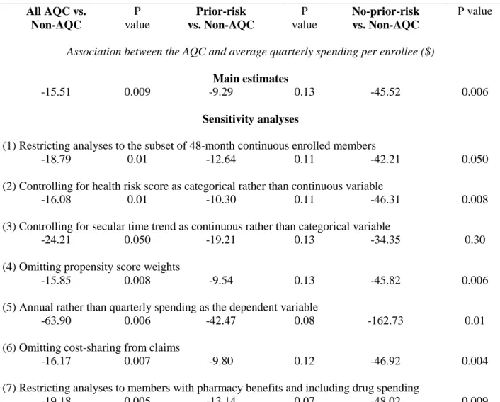
Results of sensitivity analyses support the main findings (Table 1.5). Estimates of the AQC effect on spending remain similar to the baseline case and effect sizes for the no-prior-risk subgroup remain larger than for the prior-risk subgroup. Sensitivity analyses
results support the main findings in several ways. Restricting analyses to 48-month continuously enrolled members did not alter the estimates, ameliorating adverse selection concerns. Relative savings by risk category were also unchanged after using quintiles or tertiles. Alternate controls for secular trends did not change the findings. Propensity score weights were used to balance traits between intervention and control groups, and their omission did not impact the results. Different levels of spending aggregation also produced similar results. Omitting cost-sharing from all claims did not change the estimates, suggesting that benefit design was not differentially heterogeneous among treatment and control enrollees. Finally, restricting analyses to members with pharmacy benefits with drug spending included did not change the findings. The descriptive
analyses showed that enrollees were similar in age, sex, and risk score across intervention and control groups. I also demonstrated that trends in spending prior to the intervention were not statistically different. Finally, the use of a 2-part model with logarithmic transformation and logistic models to analyze spending and quality did not change the results (not shown).
The analyses of risk trends indicate an increase in risk in the AQC group relative to the controls. This might reflect a true increase in risk, which is important to control for, or upcoding. The finding was much smaller and not statistically significant in the no-prior-risk group, which accounts for the largest savings. Nevertheless, if one assumed all of the increase in risk was due to upcoding, the AQC effect would be attenuated by between 18 to 38 percent.
Although there was an increase in risk among the AQC group, the results are likely not driven by upcoding for several reasons. First, the results are robust to
measuring risk in deciles, which would be less sensitive to upcoding. Second, the increased risk was not apparent in the no-prior-risk group, where savings is largest. Third, upcoding would presumably affect the analyses of utilization, and lead me to erroneously conclude that volumes decreased after the intervention. However, I found no AQC effect on utilization. Fourth, upcoding would likely affect both professional and facility spending and fees, but I found effects only on facility spending and fees.
Table 1.5. Sensitivity analyses of difference-in-difference estimates of the association between the AQC and health care spending.*
All AQC vs. Non-AQC P value Prior-risk vs. Non-AQC P value No-prior-risk vs. Non-AQC P value
Association between the AQC and average quarterly spending per enrollee ($) Main estimates
-15.51 0.009 -9.29 0.13 -45.52 0.006
Sensitivity analyses
(1) Restricting analyses to the subset of 48-month continuous enrolled members
-18.79 0.01 -12.64 0.11 -42.21 0.050 (2) Controlling for health risk score as categorical rather than continuous variable
-16.08 0.01 -10.30 0.11 -46.31 0.008 (3) Controlling for secular time trend as continuous rather than categorical variable
-24.21 0.050 -19.21 0.13 -34.35 0.30 (4) Omitting propensity score weights
-15.85 0.008 -9.54 0.13 -45.82 0.006 (5) Annual rather than quarterly spending as the dependent variable
-63.90 0.006 -42.47 0.08 -162.73 0.01 (6) Omitting cost-sharing from claims
-16.17 0.007 -9.80 0.12 -46.92 0.004 (7) Restricting analyses to members with pharmacy benefits and including drug spending
-19.18 0.005 -13.14 0.07 -48.02 0.009 * Main estimates are from the baseline difference-in-difference model using quarterly spending as the dependent variable, age categories, age-sex interactions, continuous risk, indicators for each quarter, and quarter*AQC interactions. The baseline model uses the sample of members
continuously enrolled for at least 12 months over the 4-year study period and uses propensity weights. Rows (1) through (7) show analogous results from sensitivity analyses. Results of the annual spending model (5) should be divided by 4 to be comparable to the quarterly estimates. All analyses use Huber-White robust standard errors.
Section 1.6.3. Decomposition of spending results into price and utilization effects.
This section details the decomposition of the difference-in-difference estimate of the association between the AQC and health care spending into its price and utilization (quantity) components. To better understand how the AQC groups achieved lower spending relative to non-AQC groups in 2009, I first repriced outpatient facility claims for each service to its median price across all providers in all 4 years of the study period. I performed repriced analysis on only outpatient facility claims because outpatient facility spending accounted for the bulk of the association between AQC and spending (see Table 1.2 and Table 1.6). Moreover, inpatient services are priced differently (diagnostic related groups or DRGs, rather than fees).
Repeating the difference-in-difference regression analyses using the repriced claims allowed me to isolate the share of spending differences due to utilization (quantity), rather than price. I found that, relative to control, the AQC was associated with a $2.62 (p=0.25) decrease in average quarterly spending per enrollee in 2009. Compared to the main estimate of a $15.51 savings associated with the AQC (decrease in spending relative to control), this repriced estimate is small and insignificant, suggesting that the main result is driven by price differences, not by utilization. Sensitivity analyses using direct measures of utilization (quantity) as the dependent variable in the model, such as the number of procedures, images, tests, admissions, or office visits, yielded no negative and significant association between the AQC and utilization. This result, however, still left two potential explanations for the price effect on spending.
Thus, I further decomposed the spending differences into two potential price-driven explanations: differential fee changes (AQC groups may have received lower fee increases than non-AQC) and referral pattern changes (AQC enrollees may have received care from lower fee providers). This was done by repricing claims to median 2009 prices for each service within each practice. This differs from the first repricing method above because it retains the variation in prices between practices, while standardizing prices
within each practice (the Massachusetts Office of the Attorney General has documented the variation in prices between practices*). The resulting association between AQC and spending reflects changes in the share of spending across practices, which I denoted the referral effect. This difference-in-difference model produced an AQC-associated relative spending decrease of $14.21 (p<0.001), which is approximately 90 percent of the main AQC-associated savings in year 1. This finding was supported by further sensitivity analyses. For example, I found no consistent differences in price trends (including hospital, non-hospital facility, and physician fees) for AQC and non-AQC providers.
* See “Examination of Health Care Cost Trends and Cost Drivers: Report for Annual Public Hearing, March 16, 2010” released by the Office of the Attorney General Martha Coakley.
Section 1.6.4.
Table 1.6. Change in average health care spending per member per quarter in AQC and non-AQC groups, prior-risk subgroup vs. control and no-prior-risk subgroup vs. control.*
Prior-risk subgroup vs. control Prior Risk AQC groups
(N=341,615)
Control Group
(N=1,351,446)
Between-Group Difference (p-value)
Pre Post Change Pre Post Change
Total quarterly spending ($) 757 816 58 781 850 69 -9.29 (0.13)
Spending by BETOS category
1. Evaluation and management 182 209 27 180 208 27 -0.25 (0.74) 2. Procedures 166 178 12 167 183 16 -4.46 (0.01) 3. Imaging 94 103 8 100 111 11 -2.80 (<0.001) 4. Test 67 75 8 74 85 11 -3.01 (<0.001) 5. Durable medical equipment 10 11 2 11 13 2 -0.16 (0.65) 6. Other 48 50 2 53 54 1 1.03 (0.66) 7. Exceptions/Unclassified 190 190 0 196 196 0 0.36 (0.93)
Spending by site and type of care
Inpatient - professional 35 37 2 34 36 2 -0.37 (0.66) Inpatient - facility 152 155 3 154 157 3 0.85 (0.83) Outpatient - professional 319 355 37 299 333 34 2.85 (0.02) Outpatient - facility 212 230 18 254 284 30 -12.16 (<0.001) Ancillary 40 39 -1 40 40 0 -0.46 (0.74) 3 0
Table 1.7.
No-prior-risk subgroup vs. control No Prior Risk AQC groups
(N=40,468)
Control Group
(N=1,351,446)
Between-Group Difference (p-value)
Pre Post Change Pre Post Change
Total quarterly spending ($) 698 725 27 791 859 68 -45.52 (0.006)
Spending by BETOS category
1. Evaluation and management 164 180 16 181 208 27 -12.38 (<0.001) 2. Procedures 154 158 4 169 185 16 -13.46 (0.003) 3. Imaging 86 92 6 101 112 11 -6.13 (0.001) 4. Test 68 70 2 75 86 11 -9.34 (<0.001) 5. Durable medical equipment 10 12 2 11 13 2 -0.17 (0.86)
6. Other 45 46 1 54 56 1 -0.09 (0.99)
7. Exceptions/Unclassified 171 168 -3 200 199 -1 -3.96 (0.72)
Spending by site and type of care
Inpatient - professional 30 30 1 34 37 2 -1.81 (0.32) Inpatient - facility 133 138 5 158 160 2 1.15 (0.91) Outpatient - professional 275 299 24 301 335 34 -11.27 (<0.001) Outpatient - facility 227 222 -5 258 287 30 -36.80 (<0.001)
Ancillary 34 37 3 41 40 0 3.21 (0.39)
* Total enrollees in prior-risk and no-prior-risk subgroups exceeds 380,142 because of enrollees who had a PCP in prior-risk and a PCP in no-prior-risk for at least one year in each case. Average spending in the non-AQC group differs slightly across Table 2 and this Section due to adjustments for age, sex, and health risk score across different sample sizes of the treatment group.
32
Section 1.6.5.
Table 1.8. Unadjusted outcome quality for BCBS and 2009 AQC Groups*
BCBS Network Average AQC Weighted Average 2007 2008 2009 2009 Diabetes
HbA1c Control (<9 percent) 83.7 79.8 82.0 80.7 LDL-C Control (<100 mg/dL) 45.7 51.3 51.3 57.7 Blood Pressure Control (130/80) 30.9 36.7 38.0 44.3
Hypertension
Controlling High Blood Pressure (140/90) 68.4 70.3 69.5 68.4
Cardiovascular Disease
LDL-C Control (<100 mg/dL) 64.2 69.5 69.5 69.9
* Outcome quality scores denote the percent of eligible enrollees for whom the quality performance threshold was met. Scores are weighted by eligible members for each measure. These scores are unadjusted averages.
33
Chapter 2
Unintended consequences of redistributing Medicare payments from
specialists to primary care physicians*
34
2.1. Introduction
Facing an imperative to control the growth of health care spending, policymakers are looking to the physician payment system for savings.1-4 The Medicare Physician Fee Schedule, which lists the prices that Medicare pays for each physician service under Part B of Medicare, faces multiple impending cuts. The recent failure of the bipartisan “super committee” to agree on a debt reduction plan triggers automatic cuts of 2 percent per year to the fee schedule beginning in 2013. Meanwhile, the sustainable growth rate formula is due to slash Medicare fees by close to 30 percent in 2013.5 Such across-the-board fee cuts are highly controversial.
As an alternative, some proposals call for lowering specialist fees while preserving or raising primary care physician (PCP) fees. The physician fee schedule contains large payment differences between primary care and specialty services, deriving from the resource-based relative value system.6,7 These fee differences have been linked to a substantial income gap between PCPs and specialists and the shortage of students entering primary care.8-11 In 2011, the Medicare Payment Advisory Commission voted to replace the sustainable growth rate system with a 10-year plan that would cut specialist payments in the Medicare fee schedule by 5.9 percent in each of the first 3 years before freezing them for the next 7, while freezing PCP fees for all 10 years.12 To date, there is little research on the effect of such asymmetric fee cuts.
On January 1, 2010, the Centers for Medicare and Medicaid Services (CMS) undertook a targeted policy to redistribute Medicare payments from specialists to PCPs by cutting specialists fees and raising PCP fees for typical physician visits. Specifically,
35
CMS eliminated payments for consultations from the fee schedule, billed more frequently by specialists, while raising fees for office visits, more frequently used by PCPs.13
Similar to consultations, physicians bill for office visits (also known as “evaluation and management”) using a set of codes that contains 5 levels of clinical complexity for both “new” patient visits (Healthcare Common Procedure Coding System (HCPCS) codes 99201-99205) and “established” patient visits (99211-99215).
Consultations had previously commanded higher payments than office visits at each level of clinical complexity. In 2009 for example, Medicare paid $124.79 on average for a consultation of medium complexity, compared to $91.97 for a new patient office visit and $61.31 for an established patient office visit of medium complexity. In place of
consultations, the 2010 policy instructed all physicians to bill for office visits. Despite the simultaneous fee increase for office visits, they remained well below prior consultation fees, with new office visits 16-26 percent lower and established office visits 42-61 percent lower than their consultation counterparts from 2009 (Section 2.6.1). The compensatory increase in office visit fees averaged about 5 percent (Section 2.6.2).
CMS designed the policy to be budget neutral—amounting to a transfer of dollars from specialists to PCPs.13 Budget neutrality was based on a CMS assumption of no “upcoding.”14
In other words, physicians were assumed to bill for office visits of the same level of complexity as they had done for prior consultation codes. I evaluated the effects of this policy on spending, volume, and intensity of coding for office encounters in the first year of implementation.
36
2.2.1. Study Population
The population consisted of Medicare beneficiaries drawn from the 2007-2010 Thomson Reuters MarketScan Medicare Supplemental claims database. This database consists of a large convenience sample of U.S. Medicare beneficiaries with Medicare Supplemental (Medigap) coverage through large employers. For all of these beneficiaries, Medicare is the primary payer and all Medicare claims are reported in the data.15
From a total of 2.9 million beneficiaries, I excluded 326,491 beneficiaries who were not enrolled for at least 1 calendar year. In addition, I excluded 311,271 subjects who were enrolled in health maintenance organization or other plans paid through capitation. Physicians for beneficiaries in capitated plans may not be directly affected by the fee schedule changes. The final analytic sample comprised 2.2 million beneficiaries who were enrolled for at least 1 year. In one of the sensitivity analyses, I further restricted the sample to 798,262 beneficiaries who were continuously enrolled for all 4 years in the data. I compared baseline characteristics of the population before and after the
intervention using t-tests for continuous variables and the Pearson Chi-squared test for categorical variables.
2.2.2. Study Design
I used an interrupted time series (segmented regression) design to estimate the effect of the Medicare policy on spending, volume, and intensity of coding for all 3 types of outpatient encounters (consultations, new patient office visits, and established patient office visits). The pre-intervention period was 2007-2009, and the post-intervention
37
period was 2010. I analyzed the policy’s effects on all encounters, as well as on each type of encounter.
In the Medicare Physician Fee Schedule, determination of the clinical complexity of a patient-physician encounter is somewhat subjective. For example, a level 1 new patient office visit is characterized by a “problem-focused” history and physical
examination involving “straightforward” medical decision-making, typically requiring 10 minutes. In contrast, a level 5 new patient office visit entails a “comprehensive” history and examination involving decision making of “high complexity,” typically requiring 60 minutes (Section 2.6.3). I examined changes in the coding of complexity associated with the policy, adjusting for actual health status, baseline trends, and other covariates.
I also decomposed the policy’s effect by provider specialty. Specifically, I assigned claims to the PCP category if provider specialty was internal medicine, family medicine, geriatric medicine, pediatrics, or preventive medicine. These providers
accounted for about half of the claims. The remaining half was assigned to the specialist category, with a small fraction of non-physicians and facility providers excluded. I used only outpatient claims and included both professional and facility fees for all encounters.
2.2.3. Empirical Approach
For the spending analysis, the dependent variable was spending (in 2010 U.S. dollars). Spending was computed from claims-level total payments, including employer and beneficiary cost sharing. For analyses of volume, the dependent variable was the number encounters. Each encounter was a unique instance of a consultation or office
38
code for a unique beneficiary on a unique day. For the complexity analysis, the dependent variable was the encounter’s level of complexity.
Independent variables included age, sex, health risk score, secular trends, indicators for quarter of the year, and indicators for the beneficiary’s hospital referral region (HRR). Taking beneficiary demographic information and ICD-9 diagnoses in the claims, I calculated health risk scores using the CMS hierarchical condition categories (CMS-HCC) model, which is used for formal risk adjustment of payments to Medicare Advantage plans.16 This model generates a risk score based on age, sex, and diagnoses. HRRs are hospital markets constructed based on where patients receive care and are commonly used in the study of geographic variations in spending and utilization.17,18 Over 90 percent of beneficiaries in Medicare live in one of the 306 HHRs where over 80 percent of residents’ care is delivered by providers in that HRR.19
Since cost sharing also affects utilization of services, I included each beneficiary’s cost sharing as a percentage of total encounter spending in the model as a sensitivity analysis. This is a unique variable in the Marketscan Medicare claims data which is not available in traditional Medicare Part B claims.
All statistical analyses were conducted at the beneficiary-quarter level. I used a multivariate interrupted time series (segmented regression) model of the following form.
yit = αit + XitП + β1trendt + β2pre2009t + β3post2010t + τt + δi + εit
The vector of individual characteristics, Xit, comprises age categories, interactions
39
linear trend over the 4 year period, a dummy variable for pre-2009 to account for an unrelated policy that increased payments in the 2009 fee schedule, and a dummy variable for post-2010 which identifies the discontinuity in the outcome variable after 2010. The coefficient β3 reflects the change in average quarterly levels of the outcome after the
policy took effect, controlling for pre-intervention trends. In other words, the model captures a discontinuity in “cell” averages in 2010 compared to before, rather than a discrete change at quarter 1 of 2010 from annual trends. The cell average model with an underlying trend is preferred over the year-to-year trend break model for two reasons. First, any volatility in annual trends can dramatically affect the treatment effect given only 4 data points for each year. Second, and more importantly, given only 1 year of post-intervention data, it is likely premature to interpret any significant coefficient on the 2010 trend as a true policy effect. Thus, the model identifies an average level change. Standard errors were clustered at the hospital referral region level, which produces even more conservative standard errors than alternative methods of individual-level
generalized estimation equation models.20,21
I conducted a number of sensitivity analyses from the baseline model, including omitting quarter fixed effects for seasonality, HRR fixed effects, secular trend, and individual beneficiary characteristics (Section 2.6.4). I also repeated analysis on the continuous 4-year enrollees, as well as repeating analysis after including of cost sharing in the model. All analyses were conducted using STATA software, version 11 (Statacorp; College Station, TX). Results are reported with two-tailed P values. The Harvard Medical School Office for Research Subject Protection approved the study protocol.
40
2.3. Results
There were 2,247,810 unique Medicare beneficiaries who were continuously enrolled for at least one year during the study period. Table 2.1 describes the age distribution, gender, CMS-HCC risk scores, and region of residence for the population before and after the 2010 policy.
Table 2.1. Characteristics of the Study Population.*
Characteristics Medicare Beneficiaries
(N=2,247,810) Before elimination of consultations (2007-09) After elimination of consultations (2010) P value Member characteristics
Mean age (yrs) 75.0 ± 7.4 75.5 ± 7.4 <0.001
Age distribution (%) <0.001 65-69 yrs 29.9 26.8 70-74 yrs 22.2 22.8 75-79 yrs 20.4 20.4 80-84 yrs 15.7 16.5 ≥85 yrs 11.7 13.4 Male sex (%) 45.1 45.5 <0.001 CMS-HCC risk score † 0.56 ± 0.20 0.52 ± 0.21 <0.001 Region of residence (%) <0.001 Northeast 14.6 14.5 North central 38.9 44.2 South 34.3 32.3 West 12.1 8.9
* Plus-minus values are mean ± SD. Variables before and after the intervention were compared using t-tests for continuous variables and the Pearson Chi-squared test for categorical variables. † The CMS-HCC risk score is the concurrent risk score calculated from age, sex, and diagnoses information using the Centers for Medicare and Medicaid Services Hierarchical Condition Category (HCC) system.
41
2.3.1. Spending
In the first year, the policy eliminated an average of $18.52 per beneficiary per quarter (95% confidence interval [CI], -$19.48 to -$17.55; p<0.001) in consultation spending. At the same time, spending increased by $13.64 (95% CI, $12.89 to $14.40; p<0.001) on new patient office visits and $15.08 (95% CI, $13.56 to $16.60; p<0.001) on established patient office visits per beneficiary per quarter. On net, spending on all physician encounters was higher by $10.20 per beneficiary per quarter after the policy, controlling for pre-existing trends (95% CI, $8.58 to $11.82, p<0.001) (Table 2.2).
These changes represented a more than doubling of spending (131 percent
increase) on new patient office visits and a 12 percent increase in spending on established visits. Spending was substantially higher at baseline for established visits than for new visits, confirming that the former comprises the majority of physician’s face-to-face encounters with patients. Net spending on all encounters increased 6 percent after the policy.
Figures 1A and 1B decomposes unadjusted monthly spending per beneficiary by category of physician specialty. Prior to the elimination of consultations, average
spending on specialist consultations was three-fold higher than that for PCPs.
Correspondingly, spending on new office visits to specialists saw a larger commiserate jump than that for PCPs in 2010 (Figure 2.1A). Spending on established patient visits increased for both PCPs and specialists after the policy (Figure 2.1B), driving an increase overall spending for both groups. The statistical model shows that 58 percent of the increased spending were attributable to PCP encounters, while 42 percent were for specialist encounters (p<0.001).