University of Mannheim / Department of Economics
Working Paper Series
Competition under Consumer Loss Aversion
Heiko Karle Martin Peitz
Working Paper 12-8
Heiko Karle
†Universit´e Libre de Bruxelles
Martin Peitz
‡University of Mannheim
Version: May 29, 2012
Abstract
We address the effect of contextual consumer loss aversion on firm strategy in im-perfect competition. Consumers are fully informed about match value and price at the moment of purchase. However, some consumers are initially uninformed about their tastes and form a reference point consisting of an expected match—value and price distribution, while others are perfectly informed all the time. We show that, in duopoly, a larger share of informed consumers leads to a less competitive outcome if the asymmetry between firms is sufficiently large and that narrowing the set of products which consumers consider leads to a more competitive outcome.
Keywords: Contextual Loss Aversion, Reference-Dependent Utility, Behavioral
In-dustrial Organization, Imperfect Competition, Product Differentiation
JEL Classification: D83, L13, L41, M37.
∗This paper merges and replaces the two previous papers “Consumer Loss Aversion and the Intensity of Competition” and “Pricing and Information Disclosure in Markets with Loss-Averse Consumers.” We are grateful to Heski Bar–Isaac, Paul Heidhues, Justin Johnson, Emir Kamenica, Rani Spiegler, and various seminar audiences for helpful comments and suggestions. We gratefully acknowledge financial support from the National Bank of Belgium (Research Grant, “The Impact of Consumer Loss Aversion on the Price Elasticity of Demand”) and the German Science Foundation (SFB TR 15).
†ECARES, Universit´e Libre de Bruxelles (ULB), B-1050 Brussels, Belgium. E-mail: [email protected] ‡Department of Economics, University of Mannheim, 68131 Mannheim, Germany. E-mail: [email protected]. Also affiliated with CEPR, CESifo, ENCORE, and ZEW.
1
Introduction
Consumer information about price and match value of products is a key determinant of market outcomes. If consumers are loss–averse, information prior to the moment of pur-chase matters: Product information plays an important role at the stage at which loss– averse consumers form expectations about future transactions.
In this paper, we investigate the competitive effects of contextual consumer loss aversion— i.e., of consumer loss aversion when prices within a product category define the context in which consumers make their consumption decision. Our theory applies to inspection goods, with the feature that consumers readily observe prices in the market but have to inspect products before knowing the match value—i.e., the fit between product character-istics and consumer tastes.1 As we argue below, this description applies to a number of
product categories and, thus, is important for understanding market interaction.
Our setup is motivated by empirical and experimental evidence in the marketing and eco-nomics literatures: consumer choice behavior is influenced by reference prices according
to a large body of evidence documented in the marketing literature (see Mazumdar, Raj, and Sinha (2005) for an overview). In particular, contextual reference prices which are based on
current prices within a product category at the moment of purchase affect consumer choice—see Rajendran and Tellis (1994). According to this view consumers feel a loss if they do not buy a cheap product within a product category. In addition, loss aver-sion in consumer choice has been widely documented in a variety of laboratory and field settings in the economics literature, starting with Kahneman and Tversky (1979). Fur-thermore, loss-averse consumers may base their reference point on rational expectations, as in K˝oszegi and Rabin (2006, 2007), and with respect to prices and match value, as formalized in Heidhues and K˝oszegi (2008). Empirical and experimental evidence on multi-dimensional, expectation–based loss aversion is provided by Crawford and Meng (2011), Ericson and Fuster (forthcoming) and Karle, Kirchsteiger, and Peitz (2011). Following the theory of K˝oszegi and Rabin (2006, 2007), we postulate that, to make
1The terminology of inspection goods was introduced by Hirshleifer (1973). Inspection goods and
observable prices are considered in Anderson and Renault (2009) and, more generally, in the clearing house literature.
their consumption choices, loss–averse consumers form their probabilistic reference point based on expected future transactions, which are confirmed in equilibrium. Here, a con-sumer’s reference point is her probabilistic belief about the relevant consumption out-come (price and product match) held between the time she first focuses on the decision determining the consumption plan—i.e., when she heard about the products in a partic-ular context, was informed about the prices for the products on offer, and formed her expectations—and the moment she actually makes the purchase.2
We distinguish between “informed” and “uninformed” consumers at the moment con-sumers form their reference point. Informed concon-sumers know their taste ex ante and will perfectly foresee their equilibrium utility from product characteristics. Therefore, they will not face a loss or gain in product satisfaction beyond their intrinsic valuation.
Ex–ante uninformed consumers, by contrast, are uncertain about their ideal product char-acteristic: They form expectations about the difference between ideal and actual product characteristic which will serve as a reference point when evaluating a product along its match–value dimension. They will also face a gain or a loss relative to their expected dis-tributions of price after learning the taste realization. Since all consumers become fully informed before making their purchasing decision, we isolate the effect of consumer loss aversion on consumption choices and abstract from the effects of differential information at the moment of purchase. Our model can be interpreted alternatively as one in which consumers know their ideal taste ex ante, but are exposed to uncertainty about product characteristics when they form their reference point.
Ex–ante uninformed consumers form expectations before knowing their match value at-tributed to a particular product, but after learning the prices of the products. This timing with respect to information release and reference–point formation appears to be the appro-priate modeling choice when price information is more easily accessible for consumers than information about product characteristics.3 This is true, in particular, if price
infor-2For evidence that expectation–based counterfactuals can affect the individual’s reaction to
outcomes, see Blinder, Canetti, Lebow, and Rudd (1998), Medvec, Madey, and Gilovich (1995), and Mellers, Schwartz, and Ritov (1999). K˝oszegi and Rabin (2006, 2007) have developed the general theory of expectation–based reference points and the notion of personal equilibrium.
3In a dynamic extension in the spirit of K˝oszegi and Rabin (2009) we would need that consumers’
expectations about prices are updated before the consumers’ expectations about match values. See the concluding section for more detail.
mation is provided at the moment consumers become aware of the existence of products, but in which match value is difficult to evaluate without closer inspection. This is arguably the case with price advertising by intermediaries such as online price comparison web-sites, when consumers are agnostic about prices prior to seeing the posted prices. Even if consumers did not observe product prices before entering the shop (or starting the in-spection), in many cases consumers first access the information in the price dimension of each product of interest and then start learning about their product–specific match values by comparing products with each other. In particular, consumers can easily interpret price differences, but need time to digest and interpret differences of product characteristics. The inspection of product characteristics of both products is assumed to happen simul-taneously. This holds trivially if consumers obtain information only from a comparison between the two products.4
Consider an initially uninformed consumer who decides which of two or more diff eren-tiated products to buy. She knows the prices of the products, e.g., because prices are advertised or easily available on a price search engine, but learns the match value only af-ter spending some time to figure out how useful the products are to her. Such uninformed consumers are likely to be present in product markets in which products are bought in-frequently and possess characteristics whose values take time to evaluate (e.g., electronic devices, holiday trips, tools, or furniture). This also applies to markets of products whose match value is only revealed later in time (e.g., transport services or cultural events sold only on the spot market for which some consumers do not initially know their opportu-nity costs for different time slots) or at the moment of inspection (e.g., perfumes for which inexperienced consumers cannot associate a brand with a particular smell).
Since consumers observe prices before forming their reference point, firms can use price as an expectation-management tool. In other words, price announcements affect not only consumer behavior given reference points, but, in addition, they endogenously change consumer preferences. If firms set different prices, uninformed consumers will face either a loss or a gain in the price dimension ex post, depending on whether they buy the more-or less-expensive product. Hence, an (ex ante) uninfmore-ormed consumer’s realized net utility
4In the same spirit, one stream of the literature on consumer search postulates that search is
depends not only on the price of the product she buys, but also on the price of the product she does not buy. By lowering its price, a firm increases the probability the consumer expects to buy the product. Thus, the firm can manage the probabilistic reference point affecting the utility function at the moment of purchase. This analogously holds also in the match-value dimension, where a price reduction increases the probability that a consumer will buy a product that does not provide such a good fit.
Analyzing the competitive effects under consumer loss aversion, we find that consumer loss aversion in the price dimension has a pro–competitive effect whereas loss aversion in the match value dimension has an anti–competitive effect. We relate the pro-competitive effect to price comparisons by consumers. In our benchmark model (symmetric duopoly with the same degree of loss aversion in the price and match–value dimension), we find that the anti–competitive effect dominates the pro–competitive one. This implies that a larger fraction of ex–ante informed consumers makes competition more intense. In other words, more widespread product information at the ex–ante stage is pro–competitive. Thus, transparency policies for new products which increase the number of informed con-sumers in the market have a pro–competitive and, hence, consumer–surplus–increasing effect.
In the main part of the paper, we show that the relative weights of the two dimensions of loss aversion are altered (1) if firms are asymmetric with respect to marginal costs or (2) if the number of firms increases and analyze the competitive effects of loss aversion in these settings. In asymmetric duopoly, we find that the price difference between the less and the more efficient firm is exacerbated through the presence of uninformed loss–averse consumers. Here, the more efficient (low–cost) firm has a strong incentive to attract those consumers by increasing the price gap. In equilibrium, the pro–competitive effect in the price dimension dominates the anti–competitive effect in the match–value dimension if the cost difference (which increases the equilibrium price difference and thus the magni-tude of loss aversion in the price dimension) is sufficiently large. An interpretation of this results is that under strong cost asymmetries with uninformed loss–averse consumers, a low–cost firm can be prominent by setting a low price. For instance, consider a low–cost private label competing with a high–cost national brand. Under strong cost asymmetries, we also predict that, in addition to releasing price information, the private label may
dis-close match–value relevant information and thus make consumers informed ex ante to mitigate price competition—we elaborate on this point in the discussion section.
In our second extension, we turn to symmetric oligopoly to investigate comparative statics in the number of firms. The comparative statics effects of varying the number of firms n are the same as those in an N-firm oligopoly when varying the size of the consumers’ con-sideration set n < N—i.e. the number of neighboring products that consumers are aware
of. For n > 2, there are multiple equilibria. Selecting the equilibrium that maximizes firm profits we show that a larger consideration set (a larger number of firms) relaxes competition. The explanation of this result is related to consumers’ initial probability of buying the product of a single firm and, hence, the probability of facing the price of a single firm. We receive that this probability is decreasing in n. Since loss aversion in the price dimension is increasing in this probability, it follows that loss aversion in the price dimension becomes less pronounced as n increases which reduces the pro–competitive effect of loss aversion (renders price comparisons less effective as n increases). In this light, product proliferation can be interpreted as a means to make price comparisons less successful and therefore less relevant. Moreover, when we interpret targeted advertising to consist in decreasing the seize of consumers’ consideration set, we find that if firms coordinate on the equilibrium that maximizes industry profits, they would be better off
from jointly agreeing not to use targeted advertising since targeted advertising intensifies competition.
In our modeling effort, we follow Heidhues and K˝oszegi (2008), who also consider en-dogenous reference points in a market setting. Our model is enriched by considering heterogeneous consumers who differ according to their knowledge of their preferences when they form their (probabilistic) reference point. Our framework has two distinguish-ing features: First, consumers and firms know the market environment; in particular, firms know the actual (possibly asymmetric) cost realizations.5 Second, consumers learn posted
prices before they form their reference points. Due to this timing, our duopoly model de-livers unique equilibrium predictions.6
5This allows us to compare our results with those in the standard Hotelling–Salop setting. By contrast,
in Heidhues and K˝oszegi (2008), costs may be private information.
In a related paper, Zhou (2011) considers competitive effects of consumer loss aversion when consumers do not base reference points on expectations but on past observations of firms’ prices and product matches. In his paper, the firm visited first (the prominent firm) may attract an excessive market share with loss–averse consumers, while in our model, the firm setting the lower price may do so. An advantage of our setup is that prominence arises endogenously due to reference pricing, whereas, in Zhou (2011), prominence is exogenous.
Heidhues and K˝oszegi (2010) and Spiegler (2011b) investigate monopoly models with consumer loss aversion. In Heidhues and K˝oszegi (2010)’s setting consumers are loss– averse with respect to prices and reservation utility from purchase and the monopolist initially commits to a price distribution depending on cost realizations. They show that consumer loss aversion with expectation–based reference points provides a rationale for sticky regular prices and variable sales for frequently purchased goods. Spiegler (2011b) reproduces their main result by using a simpler, sampling-based reference concept. Fur-thermore, he finds that loss aversion lowers expected monopoly prices and that sticky– price equilibria are more likely to arise when uncertainty stems from demand shocks rather than from costs shocks.
Herweg, Mueller, and Weinschenk (2010) and Herweg and Mierendorff(forthcoming) have applied the expectation–based loss aversion concept of K˝oszegi and Rabin (2006, 2007) to agency models. More broadly, our paper contributes to the literature on behavioral industrial organization, as surveyed in Ellison (2006), DellaVigna (2009), and Spiegler (2011a). An important issue in our paper, as in Eliaz and Spiegler (2006), is the compar-ative statics effects in the composition of the population. In their model this composition effect is behavioral in the sense that the share of consumers with a particular behavioral pattern changes. We do not resort to this interpretation, although our analysis is com-patible with it: We allow the composition effect to be informational in the sense that the arrival of information in the consumer population is changed (while the whole popula-tion is subject to the same behavioral pattern). The informapopula-tional interpretapopula-tion lends
Hence, firms can deviate from consumers expectations about prices. This creates a discontinuity in con-sumers’ marginal gain–loss utility and yields to a kinked demand curve at the expected price. The kinked demand curve leads to a non-response of prices for some cost interval (focal prices) and a multiplicity of equilibria.
itself naturally to addressing questions about the effect of early information disclosure to additional consumers.
Our paper also relates to the literature on the economics of advertising—for a survey on the economics of advertising see Bagwell (2007). It belongs to the strand that consider ad-vertising as “hard” information; in this sense we consider directly informative adad-vertising. Our paper uncovers the role of content advertising as consumer expectation management, which provides a complementary view to Anderson and Renault (2006). Since, at the point of purchase, consumers are fully informed there is no role for content advertising at the purchasing stage. Content advertising, however, can remove the uncertainty con-sumers face at the ex ante stage—i.e., when forming their reference point—and can be seen as a hybrid form of informative and persuasive advertising: It changes preferences at the point of purchase which corresponds to the persuasive view of advertising albeit due to information that is received ex ante which corresponds to the informative view of advertising. It also points to the importance of the timing of advertising: For expecta-tion management via advertising, it is important to inform consumers prior to forming their reference points.7 Our second extension also connects to the literature on targeted
advertising, as will be spelled out in Section 4.
Our paper can be seen as complementary to the work on consumer search in product markets—see, e.g., Varian (1980), Anderson and Renault (2000), Janssen and Moraga-Gonz´alez (2004), Armstrong and Chen (2009). Whereas that literature focuses on the effect of dif-ferential information (and consumer search) at the purchasing stage, our paper abstracts from this issue and focuses on the effect of differential information at the expectation-formation stage which is relevant if consumers are loss–averse.
The plan of the paper is as follows. In Section 2, we present the baseline model and establish the benchmark result that a larger share of informed consumers leads to lower prices. We then allow for different degrees of consumer loss aversion in the price and the
7Other marketing activities can also be understood as making consumers informed at the stage when
they form their reference point. For instance, test drives for cars or lending out furniture, stereo equip-ment, and the like make consumers informed early on. Arguably, in reality, uncertainty may not be fully resolved even at the purchasing stage. However, to focus our minds, we only consider the role of mar-keting activities on expectation formation before purchase. In short, in our model firms may use market-ing to manage expectations of loss–averse consumers at an early stage. For a complementary view, see Bar-Isaac, Caruana, and Cunat (2010).
match value dimension. In Section 3, we allow for cost asymmetries between firms in the baseline model. In Section 4, we allow for any finite number of firms in the benchmark model and link this to the size of the consideration sets of consumers. Section 5 provides some further discussion and Section 6 concludes. Some of the proofs are relegated to Appendix A. Tables of numerical illustration are contained in Appendix B. Appendix C contains relegated material on equilibrium existence and uniqueness. Appendix D con-tains the derivation of demand in the n-firm oligopoly. Appendix E concon-tains an extension in which consumers receive noisy signals about their match value ex ante, as discussed in Section 5.
2
The Baseline Model
2.1
Setup
Consider a duopoly market in which firm i = 1,2 incurs a constant marginal cost of pro-duction ci = c. Firms are located on a circle of length 2 with maximum distance, y1 = 0,
y2 = 1. Firms simultaneously announce prices pi to all consumers. We consider hori-zontally differentiated products `a la Salop (1979). A continuum of loss-averse consumers of mass 1 are uniformly distributed on the circle of length 2. A consumer’s location x,
x∈[0,2), represents her taste parameter. Her taste is initially—i.e., before she forms her reference point—known only to herself if she belongs to the set of informed consumers. In our model, consumers’ differential information applies to the date at which consumers determine their reference point and not to the date of purchase: A fraction (1 −β) of loss–averse consumers, 0 ≤ β ≤ 1, is initially uninformed about their taste. As will be detailed below, they endogenously determine their reference point and then, before making their purchasing decision, observe their taste parameter (which then becomes private information of each consumer). At the moment of purchase all consumers are perfectly informed about product characteristics, prices, and tastes. All consumers have the same reservation value v for an ideal variety and have unit demand. Their utility from not buying is−∞so that the market is fully covered.
We could alternatively consider competition on the Hotelling line. Our circle model is, in terms of market outcomes, equivalent to the Hotelling model in which consumers are uniformly distributed on the [0,1]-interval and firms are located at the extreme points of the interval. However, the circle model allows for an n-firm extension and for an alternative and equivalent interpretation about the type of information some consumers initially lack: At the point in time consumers form their reference–point distribution, they all know their taste parameters, but only a fraction (1 −β) does not know the location of the firms—these uninformed consumers only know that the two firms are located at maximal distance.
Various justifications for differential information at the ex–ante stage can be given. For in-stance, consumers may differ by their experience concerning the relevant product feature: Some may have previously bought the product, whereas others are new on the market. Alternatively, a share of consumers may know that they will be subject to a taste shock between forming their reference point and making their purchasing decision. These con-sumers then do not condition their reference point on the ex–ante taste parameter, whereas those belonging to the remaining share do.
To determine the market demand faced by the two firms, let the informed consumer type in [0,1], who is indifferent between buying good 1 and good 2, be denoted by ˆx(p1,p2).
Correspondingly, the indifferent uninformed consumer is denoted by ˆˆx(p1,p2). Since
market shares on [0,1] and [1,2] are symmetric, the firms’ profits are:
π1(p1,p2)= (p1−c1)[β· ˆx(p1,p2)+(1−β)· ˆˆx(p1,p2)]
π2(p1,p2)= (p2−c2)[β·(1− ˆx(p1,p2))+(1−β)·(1− ˆˆx(p1,p2))].
The timing of events is as follows.
Stage 1.) Price setting: Firms simultaneously set prices (p1, p2).
Stage 2.) Contextual reference point formation: All consumers observe prices and
b) uninformed consumers form reference–point distributions over purchase price and match value (as detailed in Subsection 2.2 below.)
Stage 3.) Inspection: Uninformed consumers observe their taste x—i.e., uncertainty is re-solved for all consumers.
Purchasing: Consumers decide which product to buy:
a) informed consumers make their purchase decisions;
b) (ex–ante) uninformed consumers make their purchase decisions, based on their utility that includes realized gains and losses relative to their reference– point distribution.
We solve for subgame–perfect Nash equilibrium where firms foresee that uninformed consumers play a personal equilibrium (at stages 2b and 3b). Personal equilibrium in our context means that consumers hold rational expectation about their final purchasing decision and behave according to them in equilibrium—for the general formalization, see K˝oszegi and Rabin (2006).
2.2
Consumer demand in the baseline model
2.2.1 Demand of informed consumers
Informed consumers ex ante observe prices and their taste parameter and, therefore, do not face any uncertainty when forming their reference point. Hence, their behavior ex post is only influenced by consumers’ expected behavior ex ante (buy from firm 1 with probability one and face match x and price p1 or buy from firm 2 with probability one
and face match 1−x and price p2). K˝oszegi and Rabin (2006) show (in their Proposition
3) that, in such an environment, it is preferable for consumers from an ex–ante point of view to hold initial plans which maximize their intrinsic utility and to follow through these plans in equilibrium (preferred personal equilibrium).8 Therefore their behavior is
8The intuition behind this result is the following: In environments without uncertainty, there exists a
continuum of initial plans (around the cutoff ˆx) which consumers will follow through ex post (personal equilibria). Since none of these plans will induce a net loss ex post, it is optimal for consumers to initially choose the plan which maximizes their intrinsic utility.
the same as in the standard Hotelling-Salop model. For prices p1 and p2, an informed
consumer located at x obtains the indirect utility ui(x,pi)= v−t|yi− x| −pi from buying product i, where t scales the disutility from distance between ideal and actual taste on the circle. The expression v− t|yi − x| then captures the match value of product i for a consumer of type x. Denote the indifferent (informed) consumer between buying from firm 1 and 2 on the first half of the circle by ˆx∈[0,1]. The informed (interior) indifferent consumer is
ˆx(p1,p2)=
(t+ p2− p1)
2t . (1)
Symmetrically, a second indifferent (informed) consumer type is located at 2−ˆx(p1,p2)∈
[1,2]. Using symmetry and the uniform distribution of x, we receive that firm 1’s demand of informed consumers is equal to ˆx(p1,p2).
2.2.2 Demand of uninformed consumers
Uninformed consumers do not know their ideal taste x ex ante and, thus, are ex ante un-certain as to which product they will buy after learning their ideal taste x: They, therefore, face ex ante uncertainty in the price and match–value dimension and form reference–point distributions in these two dimensions.
Three properties of consumer behavior are worthwhile pointing out. First, consumers have gains or losses not about net utilities but about each product “characteristic”, where price is then treated as a product characteristic. This is in line with much of the experimen-tal evidence on the endowment effect—for a discussion, see, for instance, K˝oszegi and Rabin (2006).9 Second, consumers evaluate a given product by comparing it to their reference point. Due to rational expectations this reference point may depend on the rival’s product characteristics. Third, we assume here that the gain–loss parameters are the same across dimensions.
9Gains and losses also matter in the price dimension because, even though prices are deterministic,
they can be different across firms. Hence, a consumer who initially does not know her taste parameter is uncertain at this point in time about the price at which she will buy.
The uninformed consumer will buy from firm 2 if she is located close enough to firm 2—i.e., if x ∈ [ ˆˆx(p1,p2),2− ˆˆx(p1,p2)], where ˆˆx(p1,p2) is the location of the indifferent
(uninformed) consumer we want to characterize. Hence, the uninformed consumer at x will pay p2in equilibrium with Prob[p= p2]=Prob[ ˆˆx(p1,p2)< x< 2−ˆˆx(p1,p2)] and p1
with the complementary probability. Since x is uniformly distributed on [0,2], we obtain that from an ex ante perspective p1is the relevant price with probability Prob[p= p1]= ˆˆx.
Correspondingly, the purchase at price p2 occurs with probability Prob[p = p2]= 1− ˆˆx.
This defines the reference–point distribution with respect to the purchase price p. The reference–point distribution with respect to the match value refers to the reservation value
v minus the distance between ideal and actual product variety, s ∈ [0,1], times the taste parameter t. The density of the probability distribution of the distance is denoted by g(s) = Prob(|x−yσ|= s), where the location of the firm is yσ ∈ {0,1}, and the consumer x’s
pur-chase strategy in personal equilibrium for given prices isσ∈arg maxj∈{1,2}uj(x,pj,p−j).10 The corresponding cumulative distribution function is denoted by G(s).
Consider the case ˆˆx ≥ 1/2—i.e., p1 ≤ p2 so that firm 1 has a weakly larger market
share than firm 2 also for uninformed consumers. Since at p1 , p2 some uninformed
consumers will not buy from their nearest firm, g(s) is a step function with support [0, ˆˆx].
The discontinuity of g on (0, ˆˆx) is determined by the maximum distance that consumers
are willing to accept buying the more expensive product 2, s = 1− ˆˆx, as s ≤ 1− ˆˆx holds for consumers close to either 1 or 2, while s > 1 − ˆˆx only holds for the more distant consumers of 1. Hence, the density function takes the form
g(s)= 2 if s ∈[0,1− ˆˆx] 1 if s ∈(1− ˆˆx, ˆˆx] 0 otherwise.
Analogously, for the case ˆˆx<1/2.
After uncertainty is resolved, consumers experience a gain–loss utility: The reference–
10σis a function of prices and consumer’s location x conditional on consumer’s expectation about
equi-librium outcomes which are incorporated in their two-dimensional reference–point distribution. σstates a consumer’s personal equilibrium. This equilibrium concept was introduced by K˝oszegi and Rabin (2006) and requires that behavior-generating expectations must be self-fulfilling in equilibrium.
point distribution is split up for each dimension at the value of realization in a loss part with weight λ > 1 and a gain part with weight 1. In the loss part the realized value is compared to the lower tail of the reference–point distribution; in the gain part it is com-pared to the upper tail of the reference–point distribution. Following K˝oszegi and Rabin (2006), we assume in this section a universal gain-loss function for all dimensions. For
p1 ≤ p2, the indirect utility of an uninformed consumer x∈(1− ˆˆx,1] purchasing product
1 is then given by11 u1(x,p1,p2) =(v−tx−p1)−λ·Prob[p = p1](p1− p1)+Prob[p= p2](p2− p1) −λ·t Z x 0 (x−s)dG(s)+t Z 1 x (s−x)dG(s). (2)
The first term on the right-hand side reflects the consumer’s intrinsic utility from prod-uct 1. The remaining terms capture the two hedonic dimensions in which consumers experience gains and losses. The second term captures the loss in the price (or money) dimension from not facing a lower price than p1. This term is equal to zero because p1
is the lowest price offered in the market place. The third term is the gain from not facing a higher price than p1, which is positive. Note that this gain is weighted by the
proba-bility of the complementary event (buying from firm 2). Intuitively, the realized gain in the price dimension is the larger the higher was the probability of facing the higher price
p2 at the initial stage. The last two terms correspond to the loss (gain) from not facing a
smaller (larger) distance in the taste or match-value dimension than x. Analogously, an uninformed consumer’s indirect utility from a purchase of product 2 at p2 ≥ p1 is given
by u2(x,p1,p2) =v−t(1−x)−p2 | {z } Intrinsic utility −λ·Prob[p = p1](p2− p1) | {z }
Loss from facing a higher p than p1
−λ·t
Z 1−x
0
((1−x)−s)dG(s)
| {z }
Loss due to expecting smaller distance than 1−x
+ t
Z 1
1−x
(s−(1−x))dG(s)
| {z }
Gain due to expecting larger distance than 1−x (3)
11The indifferent uninformed consumer will be located at x = ˆˆx. Therefore, (1
− ˆˆx,1] is the relevant interval for determining ˆˆx for∆p≡p2−p1≥0.
This allows us to solve a consumer’s personal equilibrium by determining the location of the indifferent uninformed consumer ˆˆx, which is implicitly given by u1( ˆˆx,p1,p2) =
u2( ˆˆx,p1,p2). Let us focus on the first half of the circle and let firm 1 be the cheaper
firm—i.e., x∈[0,1] and p2 > p1.
Lemma 1. Suppose that∆p≡ p2−p1 ≥ 0, x∈[0,1], andλ∈(1, λc] withλc = 3+2
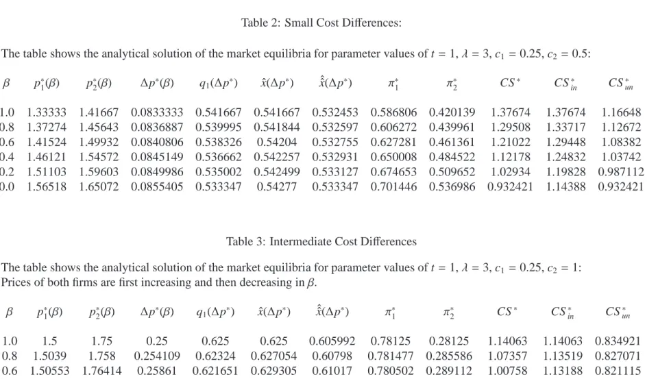
√ 5≈ 7.47. Then ˆˆx is given by ˆˆx(∆p)= λ/(λ−1)−∆p/(4t)−S (∆p), if∆p∈[0,∆˜p]; 1, if∆p>∆˜p. (4) where∆˜p≡(λ+3)t/(2(λ+1))<t and S (∆p)= s ∆p2 16t2 − (λ+2) 2t(λ−1)∆p+ (λ+1)2 4(λ−1)2. (5)
We relegate the proof of this lemma to Appendix A. For x ∈[0,1] and∆p≥ 0, the unique pure–strategy personal equilibrium of consumer x is described by
σ(x,∆p)= 1 if x∈[0, ˆˆx(∆p)] 2 if x∈( ˆˆx(∆p),1].
By symmetry and the uniform distribution of x on the circle, firm 1’s demand of unin-formed consumers is equal to ˆˆx(∆p).12 Note that ˆˆx(0) = 1/2. If∆p < 0, the location of
the indifferent uninformed consumer is given by 1− ˆˆx(−∆p) by symmetry.
12The square root S (∆p) is defined for∆p
∈[0,∆¯p] with
∆p¯≡ 2t (λ−1)
2(λ+2)−p(2(λ+2))2−(λ+1)2. (6)
∆¯p ≥∆˜p forλ∈ (1, λc]. However, forλ > λca critical price difference such thatλ/(λ
−1)−∆p/(4t)− S (∆p)=1 does not exist and we obtain a discontinuous jump up to one at∆¯p. For the sake of brevity we restrict attention to the case ofλ∈(1, λc] in the following.
2.2.3 Comparison between the demand of uninformed and informed consumers
How do ˆˆx(∆p) and ˆx(∆p) compare with one another? We can show that, for λ → 1, the indirect utility function of uninformed consumers differs from the one of informed consumers only by a constant and we obtain ˆˆx(∆p)= ˆx(∆p) as a solution in this case.
Let us compare the sensitivity of uninformed consumers’ demand with respect to price to the one of informed consumers. To do so, we define the critical price difference
∆ˆp= t 2√2·(2(λ+2))−3· p(2(λ+2))2−(λ+1)2 √ 2(λ−1) .
We obtain the following result:
Lemma 2. The demand of uninformed (or loss–averse) consumers is less price sensitive than the demand of informed consumers if the price difference is sufficiently small,∆p∈
[0,∆ˆp). The demand of uninformed (or loss–averse) consumers is more price sensitive
than the demand of informed consumers if the price difference is large,∆p∈(∆ˆp,∆˜p].
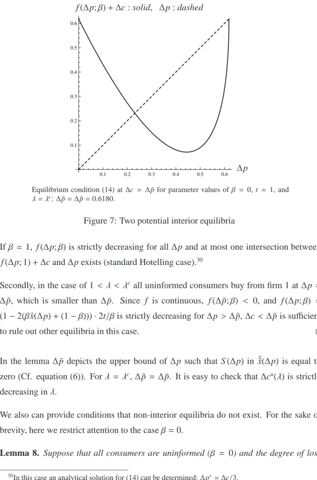
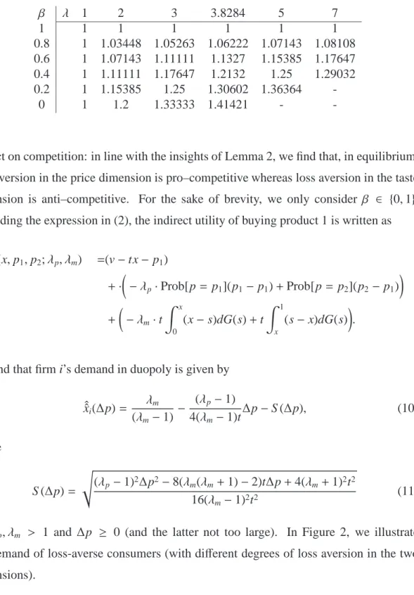
The proof of the Lemma 2 is relegated to Appendix A. Demand for uninformed vs. informed consumers is illustrated in Figure 1.13 In Section 3, we will see that this property
is a driving force for our comparative static results in asymmetric markets. We note that, at a small price difference, the indifferent uninformed loss–averse consumer is harder to attract than an informed consumer by a price decrease by firm 1 because the consumer’s net gain in the price dimension from buying at a lower price is outweighed by her net loss in the taste dimension if buying the more distant product 1. Thus, demand of loss– averse consumers reacts less sensitive to price in this range. The net gain and net loss in the two dimensions are equal to (λ−1)∆p ˆˆx(∆p) (see the difference between the second term in (20) and (21)) and−(λ−1)t(1/2−2(1− ˆˆx(∆p))2), respectively (see the difference
between the third term in (20) and (21)). Here the net gain in the price dimension is increasing and the net loss in the taste dimension is decreasing in ∆p. Moreover, both
13We restrict attention to price differences such that the indifferent consumers are strictly interior. For
larger price differences∆p∈[∆˜p,t], ˆˆx(∆p)=1, while ˆx(∆p)≤1. Then more care is needed, as is applied in Section 3.
0.1 0.2 0.3 0.4 0.5 0.6 0.7 0.6 0.7 0.8 0.9 1.0 ∆p ˆx(∆p) : dashed, ˆˆx(∆p) : solid
Location of the indifferent informed and uninformed consumer (=demand of firm 1) as a function of∆p for parameter values of t = 1 andλ = 3; thus,∆˜p = 3/4 and
∆pˆ=0.2789.
Figure 1: Demand of informed and uninformed consumers
functions are convex in ∆p. For larger price differences, ˆˆx(∆p) ∈ [1/2,1] is larger and a marginal increase in ∆p increases the net gain in the price dimension more than for
small price differences, while the net loss in the taste dimension decreases less than at lower price differences since 1 − ˆˆx(∆p) is closer to zero than to 1/2. The intuition for this finding is that, for larger price differences, the consumer is less likely to buy from the more expensive firm 2 and, thus, the avoided loss in the price dimension if not doing so ex post becomes larger. This effect dominates the reduced gain in the price dimension of buying from the cheaper firm 1 ex post which is caused by the higher probability of buying from firm 1. In addition, assigning a higher probability of buying from the more distant firm 1 leads to an expected taste difference which reduces the consumer’s loss in the taste dimension if doing so ex post. Thus, the indifferent uninformed consumer as a function of the price difference is convex. For sufficiently large asymmetries, the indifferent informed consumer is closer to the center than her uninformed counterpart. Thus, the low-price firm is better able to serve uninformed than informed consumers and it becomes “prominent´´ among uninformed consumers.
2.3
Equilibrium and comparative statics
Our framework allows us to explicitly solve for equilibrium markup in symmetric duopoly, in contrast to Heidhues and K˝oszegi (2008). The following lemma characterizes the sym-metric equilibrium.
Lemma 3. Any equilibrium is unique and symmetric. Equilibrium prices are given by
p∗i =c+ t
1− (1−2β)((λλ−+1)1),i
=1,2. (7)
Proof. Rearranging the first-order conditions of profit maximization and using that qi(0;β)= 1/2 for allβ, we obtain
p∗i −c= 1 2 q′ i(0;β) ,i= 1,2, (8) where q′i(0;β)=−1 4t(1−3β)− (1−β) 2(S (0)) 0− (λ+2) 2t(λ−1) ! =−1 4t(1−3β)+ (1−β) 22(λλ+1 −1) (λ+2) 2t(λ−1) ! = 1 4t(λ+1) 2(λ+1)−(1−β)(λ−1) .
Substituting into equation (8) yields the unique symmetric equilibrium price in (7).
As shown in Appendix C.1, for allβa symmetric equilibrium exists if and only if
1< λ≤ λc ≡1+2√2≈ 3.828 (9)
In the existence proof, we have to deal with the fact that profit functions are not globally quasi-concave, since the low–price firm’s profit becomes increasingly convex due to the
increasing convexity of its demand with loss-averse consumers. This violation of quasi-concavity reflects that the low–price firm may have an incentive to non-locally undercut to gain the entire demand of loss-averse consumers when the initial situation has the property that∆p is large. To deal with the non–quasi–concavity of the profit function of the low–
price firm, we determine critical levels for the degree of loss aversion such that no firm has an incentive to non-locally undercut. There we use that the convexity of the low–price firm’s profit function is increasing in∆p which yields that stealing the entire demand of
loss-averse consumers is the only potentially optimal deviation of the low–price firm. We define the equilibrium markup as m∗ ≡ p∗−c. Using Lemma 3, we obtain comparative
static results. In particular, as the share of informed consumers increases, each firm’s markup decreases. This result follows directly from differentiating (7) with respect toβ:
Proposition 1. Forλ ∈ (1,1+2√2], equilibrium markup is decreasing in the share of
informed consumersβ.
In other words, uninformed loss-averse consumers exert a negative external effect on in-formed consumers. This contrasts the findings of a positive external effect in Gabaix and Laibson (2006) who consider a market in which only a fraction of consumers are knowledgeable about their future demand of an “add-on service”, while other consumers are “naively” unaware of this.
For illustration, Table 1 reports equilibrium markups for different values of the share of informed consumersβand of the degree of loss aversionλ. At the upper bound ofλ,λ=
λc, the equilibrium markup reaches its maximum level of 1.414 when all consumers are loss averse. This level lies 41.4% above the level with informed (or standard) consumers.
2.4
A More Flexible Symmetric Duopoly Model
So far we imposed symmetry across the price and match value dimension. In particular, we postulated that the degrees of loss aversion are the same in the two dimensions. In this subsection, we allow for different degrees of loss aversion λp, λm ≥ 1 in the two dimensions and verify that loss aversion in each of the two dimensions has a different
Table 1: Symmetric Equilibrium: Markups β λ 1 2 3 3.8284 5 7 1 1 1 1 1 1 1 0.8 1 1.03448 1.05263 1.06222 1.07143 1.08108 0.6 1 1.07143 1.11111 1.1327 1.15385 1.17647 0.4 1 1.11111 1.17647 1.2132 1.25 1.29032 0.2 1 1.15385 1.25 1.30602 1.36364 -0 1 1.2 1.33333 1.41421 -
-impact on competition: in line with the insights of Lemma 2, we find that, in equilibrium, loss aversion in the price dimension is pro–competitive whereas loss aversion in the taste dimension is anti–competitive. For the sake of brevity, we only consider β ∈ {0,1}. Extending the expression in (2), the indirect utility of buying product 1 is written as
u1(x,p1,p2;λp, λm) =(v−tx− p1) +· −λp·Prob[p= p1](p1− p1)+Prob[p= p2](p2−p1) + −λm·t Z x 0 (x−s)dG(s)+t Z 1 x (s−x)dG(s) .
We find that firm i’s demand in duopoly is given by ˆˆxi(∆p)= λm (λm−1) − (λp−1) 4(λm−1)t ∆p−S (∆p), (10) where S (∆p)= s (λp−1)2∆p2−8(λm(λm+1)−2)t∆p+4(λm+1)2t2 16(λm−1)2t2 (11)
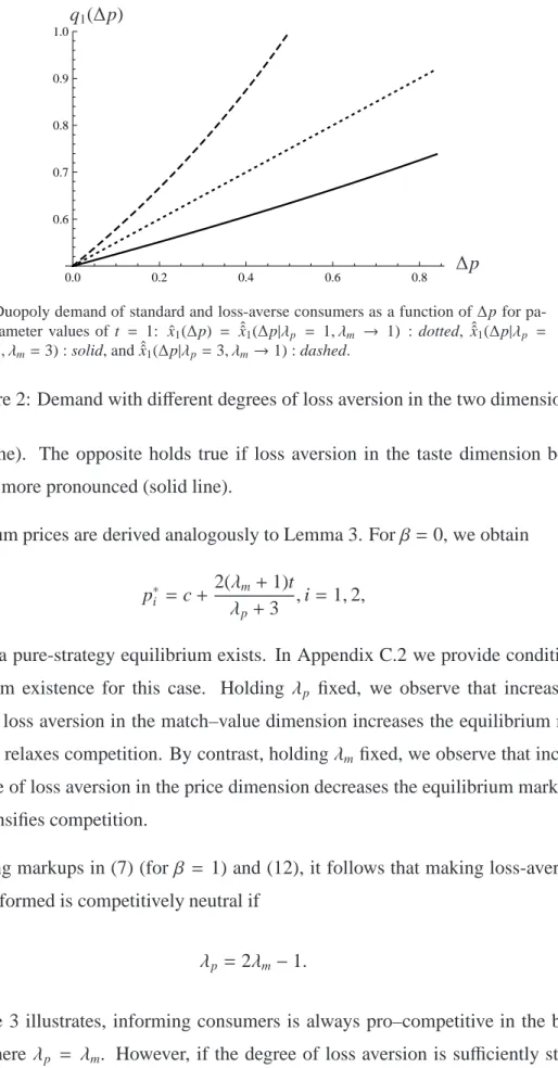
for λp, λm > 1 and ∆p ≥ 0 (and the latter not too large). In Figure 2, we illustrate the demand of loss-averse consumers (with different degrees of loss aversion in the two dimensions).
If loss aversion in the price dimension becomes relatively more pronounced (dashed line in Figure 2), then the price sensitivity of demand increases relative to the standard case
0.0 0.2 0.4 0.6 0.8 0.6 0.7 0.8 0.9 1.0 ∆p q1(∆p)
Duopoly demand of standard and loss-averse consumers as a function of∆p for pa-rameter values of t = 1: ˆx1(∆p) = ˆˆx1(∆p|λp = 1, λm → 1) : dotted, ˆˆx1(∆p|λp =
1, λm=3) : solid, and ˆˆx1(∆p|λp=3, λm→1) : dashed.
Figure 2: Demand with different degrees of loss aversion in the two dimensions (dotted line). The opposite holds true if loss aversion in the taste dimension becomes relatively more pronounced (solid line).
Equilibrium prices are derived analogously to Lemma 3. Forβ=0, we obtain
p∗i =c+ 2(λm+1)t
λp+3
,i=1,2, (12)
provided a pure-strategy equilibrium exists. In Appendix C.2 we provide conditions for equilibrium existence for this case. Holding λp fixed, we observe that increasing the degree of loss aversion in the match–value dimension increases the equilibrium markup and, thus, relaxes competition. By contrast, holdingλmfixed, we observe that increasing the degree of loss aversion in the price dimension decreases the equilibrium markup and, thus, intensifies competition.
Comparing markups in (7) (forβ = 1) and (12), it follows that making loss-averse con-sumers informed is competitively neutral if
λp =2λm−1. (13)
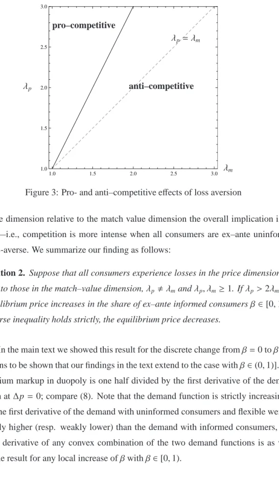
As Figure 3 illustrates, informing consumers is always pro–competitive in the baseline model where λp = λm. However, if the degree of loss aversion is sufficiently strong in
1.0 1.5 2.0 2.5 3.0 1.0 1.5 2.0 2.5 3.0 λp λm λp= λm pro–competitive anti–competitive
Figure 3: Pro- and anti–competitive effects of loss aversion
the price dimension relative to the match value dimension the overall implication is the reverse—i.e., competition is more intense when all consumers are ex–ante uninformed and loss-averse. We summarize our finding as follows:
Proposition 2. Suppose that all consumers experience losses in the price dimension dif-ferently to those in the match–value dimension,λp , λm andλp, λm ≥1. Ifλp >2λm−1,
the equilibrium price increases in the share of ex–ante informed consumersβ∈ [0,1]. If
the reverse inequality holds strictly, the equilibrium price decreases.
Proof. In the main text we showed this result for the discrete change fromβ =0 toβ= 1. It remains to be shown that our findings in the text extend to the case withβ∈(0,1)]. The equilibrium markup in duopoly is one half divided by the first derivative of the demand function at∆p = 0; compare (8). Note that the demand function is strictly increasing in
∆p. If the first derivative of the demand with uninformed consumers and flexible weights
is weakly higher (resp. weakly lower) than the demand with informed consumers, then the first derivative of any convex combination of the two demand functions is as well.
3
Cost Asymmetries
In this section, we consider asymmetric markets and provide comparative statics results with respect toβ, the share of initially informed consumers. In other words, we investigate the effects of ex ante match information on market outcomes in markets with asymmetric marginal costs c1≤ c2.
We obtain the market demand of firm 1 as the weighted sum of the demand by informed and uninformed consumers,
q1(∆p;β)=β· ˆx(∆p)+(1−β)· ˆˆx(∆p)
≡φ(∆p;β)
The demand of firm 1 is a function of the price difference∆p, which is kinked at∆˜p =
(λ+3)t/(2(λ+1)) with∆˜p< t forλ >1. Furthermore, it approaches one as∆p approaches t.14 Firm 2’s demand is determined analogously by q
2(∆p;β)= 1−q1(∆p;β). We focus
on interior equilibria in which both products are purchased by a strictly positive share of uninformed consumers—i.e.,∆p is less than∆˜p. This holds in industries in which firms are not too asymmetric.
The derivative of firm 1’s demand with respect to β expresses how demand changes as the share of ex–ante informed consumers is increased. It is the difference between the demand of informed and uninformed consumers:
∂φ(∆p;β) ∂β ≡φβ = ˆx(∆p)− ˆˆx(∆p)= 3 4t∆p− λ+1 2(λ−1) +S (∆p)≷ 0,
withφβ = 0 at∆p = 0 and∆p = t/2.This derivative can be of positive or negative sign.
As the following lemma implies, demand is decreasing in own price and increasing in the competitor’s price.
14At∆p =t, firm 1 serves also all distant informed consumers which are harder to attract than distant
uninformed consumers because the former do not perceive an overwhelming loss in the price dimension if buying from the more expensive firm 2. At∆p=t, the demand of firm 1 has another kink. We ignore the region∆p>t since we are interested in cases in which both firms face strictly positive demand.
Lemma 4. For β < 1, the demand of firm 1, q1(∆p;β) = φ(∆p;β), is strictly increasing
and convex in∆p for 0≤∆p≤∆˜p.
The proof follows directly from the properties of ˆˆx and ˆx in Section 2. In the remainder, we often refer to φ as a short-hand notation for φ(∆p;β). The derivative ∂φ/∂(∆p) is
denoted byφ′.
At the first stage, firms foresee consumers’ purchase decisions and set prices simultane-ously to maximize profits. This yields first-order conditions
∂πi
∂pi
= qi+(pi−ci)∂∂qpi
i =0 ,i= A,B
If the solution has the feature that demand of each group of consumers, informed and uninformed, is strictly positive, first-order conditions can be written as
∂π1 ∂p1 = φ−(p1−c1)φ′ =0 (FOC1) ∂π2 ∂p2 = (1−φ)−(p2−c2)φ′ =0. (FOC2)
We refer to a solution characterized by these first-order conditions as an interior solution. Since the profit function of the low-cost firm is not quasi-concave, we cannot use standard results to establish equilibrium existence.15 We rule out non-interior solutions and show equilibrium existence in Appendix C.3. In asymmetric markets, existence requires an adjustment of the upper bound of the degree of loss aversion to cost differences.
We now turn to the characterization of interior equilibria (p∗
1,p∗2).
Lemma 5. In an interior asymmetric equilibrium with equilibrium prices (p∗
1,p∗2), the
15Anderson and Renault (2009) face an, at first glance, similar fixed point problem. They consider a
general differentiated product Bertrand duopoly with covered markets in which asymmetries arise due to quality differences between firms. The authors show uniqueness and existence of a pure–strategy price equilibrium under the assumption of strict log-concavity of firms’ demand. Although strict log-concavity allows for some convexity of demand, in our setup this property is not met since for large price differences and a high degree of loss aversion the convexity of the low-price firm’s demand rises above any bound—i.e., φ′′(∆p)→ ∞for∆p→∆p and˜ λ→λc.
price difference∆p∗ = p∗
2− p∗1satisfies
∆p∗ = ∆c+ f (∆p∗;β), (14)
where∆c= c2−c1and f (∆p;β)= (1−2φ)/φ′.
Proof. Combining (FOC1) and (FOC2) yields the required equilibrium condition as a
function of price differences.
Thus, (14) implicitly defines the equilibrium price difference ∆p∗ as a function of the
parameters∆c,β,λ, and t, where the latter two parameters affect the functional form of f viaφ.
For any ∆c > 0, it is not possible to obtain explicit analytical solutions to equilibrium prices—see Appendix B for numerical solutions at particular parameter values. Never-theless, we obtain the following analytical comparative statics results.
Proposition 3. Suppose that firm 1 is the more efficient firm, c1< c2.
a) The equilibrium price difference ∆p∗(β) is decreasing in the share of informed
con-sumersβ.
b) The equilibrium price of the low-cost firm p∗1(β) is monotone or inversely U-shaped in
the share of informed consumersβ. In particular, p∗1(β) may be globally increasing
inβ.
c) The equilibrium price of the high-cost firm p∗
2(β) is monotone or inversely U-shaped in
the share of informed consumersβ. In particular, p2∗(β) may be globally increasing
inβ.
The proof is relegated to the Appendix A. In the following, we discuss the implications of this proposition. Price tends to be decreasing inβfor a small cost difference (since the markup is higher with uninformed, loss–averse consumers in this case) and increasing for a large cost difference (since the markup is lower with uninformed, loss–averse consumers in this case). In addition, a larger share of uninformed, loss–averse consumers leads to
a larger price difference.16 We observe that, in strongly asymmetric markets, lack of ex–
ante information amplifies the asymmetry in market share and price between firms. In other words, relative price and market share of the “prominent” firm is larger than in a setting in which consumers are fully informed ex ante. This implies that, with loss– averse consumers, setting a low price (and making consumers aware of this) provides a means for a low–cost firm to become prominent in a market—compare the literature on prominence in search markets, in particular, Armstrong, Vickers, and Zhou (2009). Possible examples are the presence of private labels in the food or non–food grocery industry in the U.S. (Steiner 2004, p. 115) or of low–cost holiday trip providers such as Neckermann in Europe.
Firms have to trade–off the business–stealing effect with the effect on the profit margin. This trade-offis affected by the share of informed consumers which, in many markets, can be considered to be increasing over time. We find that the price of the high–margin (i.e., low–cost) firm is monotone (i.e., globally increasing or decreasing) or inverse U-shaped in
β, depending on the parameter constellation:17 in strongly asymmetric markets (when the
effect of loss aversion is pro–competitive) the price of the low–cost firm may be increasing over time if more consumers become informed as the market matures. In these markets, we predict that a low–cost firm prefers to use low introductory prices. This describes a novel rationale for low introductory prices in the absence of quality differences. This is distinct from the classical result in Nelson (1970) where low introductory prices signal high product quality and other explanations on dynamic consumer behavior. By contrast, the price of the low–cost firm decreases over time in moderately asymmetric markets
16This is in contrast to one of the main findings in Heidhues and K˝oszegi (2008) who show that, in their
setting, consumer loss aversion is a rationale for focal prices. In Heidhues and K˝oszegi (2008) consumers do not observe prices before forming their two-dimensional reference–point distribution. Firms therefore can deviate from consumers expectations about prices. This creates a discontinuity in consumers’ marginal gain–loss utility and yields to a kinked demand curve at the expected price. The kinked demand curve leads to price rigidities for some cost interval and a multiplicity of equilibria. This discontinuity does not arise in our duopoly model since prices are observed ex ante and consumers hold correct expectations also off
equilibrium. In absence of consumer loss aversion, firms would condition prices on their marginal costs. Using our terminology, Heidhues and K˝oszegi compare a setting with mass 1 of uninformed consumers— i.e., β = 0, to a setting with mass 0 of uninformed consumers, which corresponds to a world without consumer loss aversion. The message by Heidhues and K˝oszegi (2008) is that consumer loss aversion tends to lead to (more) equal prices; our finding, by contrast, says that consumer loss aversion leads to a larger price difference in a market with asymmetric firms.
17For instance, Krishnan, Bass, and Jain (1999) report that price of color TVs and clothes dryers are
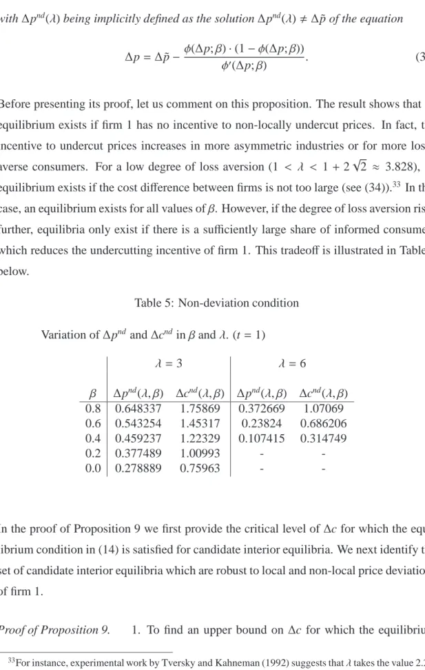
0.2 0.4 0.6 0.8 1.0 0.8 1.0 1.2 ∆c m∗ 1(∆c;β) β=0 β=1 0.2 0.4 0.6 0.8 1.0 0.8 1.0 1.2 ∆c m∗ 2(∆c;β) β=0 β=1
Equilibrium markups of firm 1 and 2 for markets in which either all consumers are uninformed (β = 0) or informed (=benchmark case, β = 1) as a function of cost differences∆c for parameter values of t=1 andλ=2.5:∆cnd(β=0)=1.27681.
Figure 4: Equilibrium markup of both firms
(when the effect of loss aversion is anti–competitive). Here, low introductory prices are not chosen by the low-cost firm.
The findings for the extreme cases β = 0 and β = 1 can be inferred from Figure 4— compare firm 1’s markups at low, intermediate, and high cost differences. The critical price difference (that implies the critical cost difference) at which price locally does not respond toβ(c.p. ∆p—i.e., the partial effect) can be solved for analytically. The critical
∆p is a function ofλand t and is independent ofβ:
∆p|∂p1 ∂β=0 (λ,t) = t 4(3+5λ) (9−(26−15λ)λ)+ √3· | −1+5λ|p(2(λ+2))2−(λ−1)2
For example, for parameters λ = 3 and t = 1 the critical price difference, at which the price of the low-cost firm reaches its maximum, satisfies ∆p|∂p1
∂β=0
(3,1) = 0.2534. It is also insightful to evaluate the derivative in the limit asβ turns to 1. In this case, we can also solve analytically for a critical ∆p at which the total derivative of p1 is zero—i.e.,
d p∗ 1(∆p∗(β);β) dβ = 0: ∆p|d p1 dβ=0 (λ,t) = t3(λ(31λ+42)−41)− √ 21· |7−11λ|√(λ+3)(3λ+5) 2(λ−3)(9λ−1) atβ=1. In the example,∆p|d p1 dβ=0
(3,1)= 7/26=0.2692 atβ= 1. This means that, given parame-tersλ= 3 and t= 1, if the equilibrium price difference satisfies∆p∗(1) <0.2692 a small decrease in the share of informed consumers leads to a higher price of the more efficient
firm, d p∗
1/dβ < 0. By contrast, for ∆p∗(1) > 0.2692, the reverse inequality holds—i.e.,
d p∗
1/dβ > 0.
For the high-cost firm, our result is qualitatively similar: The price tends to be decreasing inβfor small cost differences and increasing for large cost differences.18
We briefly discuss the firms’ incentives to disclose information—i.e., we investigate the effect of β on profits. Here, private information disclosure can be seen as the firms’ management of consumer expectations (i.e., reference points). Note that in our simple setting information disclosure by one firm fully reveals the information of both firms since consumers make the correct inferences from observing the match value for one of the two products. We confine attention to a numerical example. The critical value of
∆p such that dπ1/dβ = 0 at β = 1 and λ = 3 and t = 1, c1 = 0.25, and c2 = 1 is
∆p=0.2581. The critical value of∆p such that dπ2/dβ =0 at the same parameter values
as above is ∆p = 0.2870. The critical value at β = 1 is∆p∗(1) = 0.25 (see Table 3 in Appendix B). Hence, the critical values of∆p atβ <1 are larger than∆p∗(1). Moreover,
∆p|d p2
∂β=0
>∆p|d p1
∂β=0
.
Our numerical example shows that there are cases where increasing the initial share of ex–ante informed consumers, first none, then one and then both of the firms gain from in-formation disclosure. Since disclosing inin-formation about match value to a positive num-ber of consumers is profitable, such a strategy will be chosen by profit–maximizing firms (if disclosure is not too costly). This also implies that, for sufficiently large cost asym-metries, a “prominent” firm might disclose product match information to consumers at an
18With respect to firm 1, we also solve for critical values at which the marginal effect of firm 2’s price
changes sign: ∆p|∂p2 ∂β=0 (λ,t) = t 2(λ+1)(λ+7) (−23+(λ−10)λ)+|5−λ|p(2(λ+2))2−(λ−1)2 For instance,∆p|∂p2 ∂β=0
(3,1)=0.3201. Atβ=1 we can solve analytically for a critical∆p at which the total derivative of p2is zero—i.e., (d p∗2(∆p∗(β);β))/dβ=0: ∆p|d p2 ∂β=0 (λ,t) = t3(λ(17λ+6)−55)− √15· |11−7λ|√(λ+3)(3λ+5) 4λ(3λ−11) We have∆p|d p2 ∂β=0
(3,1) =1/2·(5√35−29) = 0.2902 at β= 1. Thus, for∆p∗(1) < 0.2902, we obtain d p2/dβ < 0 atβ=1−ǫ, while, for∆p∗(1)>0.2902, we obtain d p2/dβ > 0 atβ=1. Thus, the overall
early stage. In this case, the “prominent” firm prefers to give up a higher market share with uninformed consumers in favor of higher markups with informed consumers. This result shows that if competition becomes too intense it can become profitable for private labels (low–cost firms) to disclose product information. Our finding provides a rationale for truthfully advertising product characteristics at an early stage, although all consumers would learn them prior to purchase even in the absence of advertising. Without consumer loss aversion it would be irrelevant for market demand and market outcomes whether or not a firm advertises product characteristics ex ante.
While the focus of our analysis has been on the effect of a change of the share of ex–ante informed consumers, we may also want to compare markets with different asymmetries between firms. For this purpose, we state a comparative statics result with respect to the degree of cost asymmetry—i.e., the level of∆c= c2−c1.
Proposition 4. The equilibrium price difference∆p∗(∆c, β) is an increasing function of
the cost asymmetry between firms,∆c. It reacts more sensitive to∆c than in a market in which all consumers are informed ex ante, d(∆p∗)/d(∆c)>1/3 forβ >0.
The proof is relegated to Appendix A.2. Proposition 4 says that the more pronounced the cost asymmetry the larger the price difference between high-cost and low-cost firm. The marginal effect of an increase in cost differences on price variation is stronger if some loss-averse consumers are uninformed. We thus predict exacerbated price variation in markets with uninformed loss–averse consumers in response to a larger asymmetry. Intuitively, the more efficient firm (firm 1) is tempted to use consumer expectation management to increase its market share or prominence: announcing a very low price ex ante makes loss– averse consumers more reluctant than standard consumers to buy from the less efficient firm (firm 2) later on.
Finally, we would like to comment on the equilibrium markup of the low-cost firm m∗
1(∆c)≡
p∗
1(∆c,c1)− c1. While in the standard Hotelling world with only informed consumers
(β = 1) the markup of the more efficient firm is increasing in the cost difference, a local increase of the cost difference may have the reverse effect under consumer loss aversion
(β < 1, λ > 1). This holds true in strongly asymmetric markets: The price sensitivity
the price dimension. We note that, under very large cost differences, firm 1’s markup might fall below its level in the standard Hotelling world, as has been illustrated in Figure 4—see, also, Tables 3 and 4 in Appendix B.
4
Consideration Sets
In this section, we introduce consideration sets and focus on comparative statics with respect to the size of this set. To this effect we analyze a symmetric oligopoly. For expositional reasons, we only consider the situations in which none or all consumers are ex–ante informed, i. e. β ∈ {0,1}. We consider comparative statics in the number of firms in an n-firm oligopoly and argue that this is equivalent to varying the size of the consideration set for a given number of firms N > n in the industry. Suppose that
the length of the circle is L = n (while the consumer mass is equal to 1); this implies
that the equilibrium markup in the model with standard consumers (as in Salop (1979)) is independent of the number of firms, as additional firms do not affect the degree of product differentiation between any direct neighbors. Hence, we are able to isolate the role played by consumer loss aversion as any change in the equilibrium markup is due to the presence of consumer loss aversion. Furthermore, we observe that, under the alternative timing proposed by Heidhues and K˝oszegi (2008) that consumers form reference points before observing prices, the set of symmetric equilibrium prices is independent of the number of firms. The reason is that consumers expect a particular reference point distribution which is independent of the number of firms as a local price change given these reference points has the same effect on a firm’s demand independent of the number of firms in the market. Thus, any comparative statics results in the number of firms are due to the fact that price changes are observed initially and, thus, affect the reference–point distribution.
As shown in Appendix D, firm i’s demand n ˆˆxi(∆p,p′) for a small price decrease that does not steal any adjacent market ( ˆˆxi ∈ [1/n,2/n], pi ≤ p′, and pj = p′ for all j , i;
∆p≡ p′−p i) satisfies ˆˆxi(∆p,p′)= 4 (λ−1)(n+2) + 3n+2 n(n+2) − 2∆p n(n+2)t −2S (∆p), (15)
where
S (∆p)=
s
∆p2(λ−1)2−(λ−1)(λ(3n+2)+n(2n+5)−2)t∆p+(1+λ)2n2t2
(λ−1)2 2n+n22t2 (16)
forλ >1 and∆p≥0 and sufficiently small. Firm i’s demand for a sufficiently small price
increase can be derived analogously. Moreover, its demand for a larger price decrease is reported in the n–firm existence proof provided in Appendix C.4.
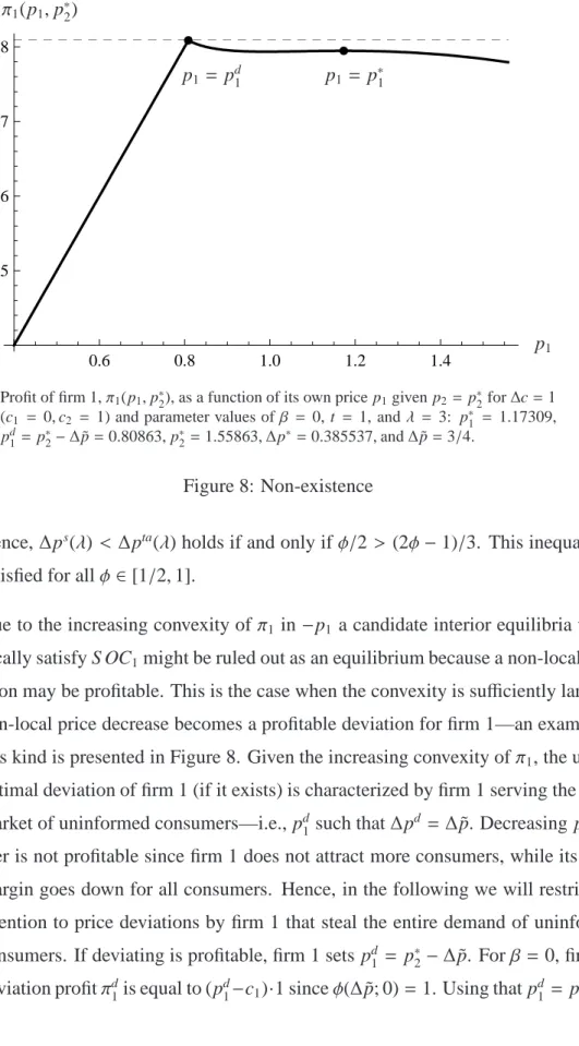
We observe that, at symmetric prices of the firm j, i, firm i’s demand is kinked for n> 2. This means that demand in oligopoly with more than two firms behaves qualitatively differently than duopoly demand because setting a slightly lower price than the competitor leads to a different marginal effect in absolute value than setting a slightly higher price if there is more than one competitor.19


![Figure 5: Location of the indifferent, loss-averse consumer (n = 2, 100) 1. for all λ ∈ (1, λ c ] with λ c = 1 + 2 √](https://thumb-us.123doks.com/thumbv2/123dok_us/1158276.2655163/33.918.203.673.100.959/figure-location-indifferent-loss-averse-consumer-λ-λ.webp)