ISSN 2042-2695
CEP Discussion Paper No 1449
October 2016
Aggregate Recruiting Intensity
Alessandro Gavazza
Simon Mongey
Giovanni L. Violante
Abstract
We develop a model of firm dynamics with random search in the labor market where hiring firms exert recruiting effort by spending resources to fill vacancies faster. Consistent with micro evidence, in the model fast-growing firms invest more in recruiting activities and achieve higher job-filling rates. In equilibrium, individual decisions of hiring firms aggregate into an index of economy-wide recruiting intensity. We use the model to study how aggregate shocks transmit to recruiting intensity, and whether this channel can account for the dynamics of aggregate matching efficiency around the Great Recession. Productivity and financial shocks lead to sizable pro-cyclical fluctuations in matching efficiency through recruiting effort. Quantitatively, the main mechanism is that firms attain their employment targets by adjusting their recruiting effort as labor market tightness varies. Shifts in sectoral composition can have a sizable impact on aggregate recruiting intensity. Fluctuations in new-firm entry, instead, have a negligible effect despite their contribution to aggregate job and vacancy creations.
Keywords: Aggregate Matching Efficiency, Firm Dynamics, Macroeconomic Shocks, Recruiting Intensity, Unemployment, Vacancies.
This paper was produced as part of the Centre’s Labour Markets Programme. The Centre for Economic Performance is financed by the Economic and Social Research Council.
Acknowledgements
We thank Steve Davis, Jason Faberman, Mark Gertler, Bob Hall, Leo Kaas, Ricardo Lagos, and Giuseppe Moscarini for helpful suggestions at various stages of this project, and our discussants Russell Cooper, Kyle Harkenoff, William Hawkins, Jeremy Lise and Nicolas Petrosky-Nadeau for many useful comments.
Alessandro Gavazza, London School of Economics, Centre for Economic Performance and CEPR. Simon Mongey, New York University. Giovanni L. Violante, New York University, CEPR, IFS, IZA and NBER.
Published by
Centre for Economic Performance
London School of Economics and Political Science Houghton Street
London WC2A 2AE
All rights reserved. No part of this publication may be reproduced, stored in a retrieval system or transmitted in any form or by any means without the prior permission in writing of the publisher nor be issued to the public or circulated in any form other than that in which it is published.
Requests for permission to reproduce any article or part of the Working Paper should be sent to the editor at the above address.
1
Introduction
A large literature documents cyclical changes in the rate at which the US macroeconomy matches job seekers and employers with vacant positions. Aggregate matching efficiency, mea-sured as the residual of an aggregate matching function that generates hires from inputs of job seekers and vacancies, epitomizes this crucial role of the labor market.
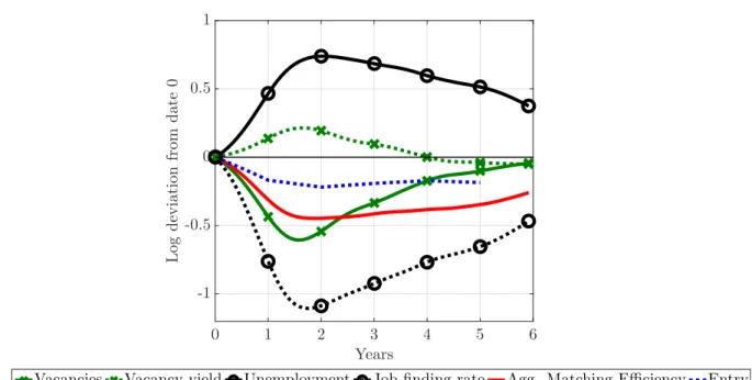
The Great Recession represents a particularly stark episode of deterioration in aggregate matching efficiency. Our reading of the data, displayed in Figure 1, is that this decline con-tributed to a depressed vacancy yield, to a collapse in the job finding rate and to persistently higher unemployment following the crisis. Identifying the deep determinants of aggregate matching efficiency is therefore necessary for a full understanding of the labor market dynam-ics during that period.
A number of explanations have been offered for the decline in aggregate matching efficiency around the recession, virtually all of which have emphasized the worker side.1 A shift in the composition of the pool of job seekers towards the long-term unemployed, by itself, goes a long way towards explaining the drop (Hall and Schulhofer-Wohl, 2013); however as documented by Mukoyama, Patterson, and ¸Sahin (2013), workers’ job search effort is counter-cyclical and tends to compensate compositional changes. Hornstein and Kudlyak(2015) include both mar-gins in their rich measurement exercise and conclude that they offset each other almost per-fectly, leaving the entire drop in match efficiency from unadjusted data to be explained. A rise in occupational mismatch shows more promise, but it can account for at most one third of the drop and for very little of its persistence (¸Sahin, Song, Topa, and Violante,2014).
The alternative view we set forth in this paper is that fluctuations in the effort with which firms try to fill their open positions affect aggregate matching efficiency. When aggregated over firms, we call this factor aggregate recruiting intensity. Our goal is to investigate whether
this is an important source of the dynamics of aggregate matching efficiency, and to study the economic forces that shape how it responds to macroeconomic shocks.
Our main motivation is the empirical analysis of recruiting intensity at the firm level in Davis, Faberman, and Haltiwanger(2013) (henceforthDFH)—the first paper to rigorously use
1A notable exception is the model inSedláˇcek(2014) that generates endogenous fluctuations in match efficiency
Figure 1: Labor market dynamics around the Great Recession (2008:01 - 2014:01) 0 1 2 3 4 5 6 Years -1 -0.5 0 0.5 1 L o g d ev ia ti o n fr o m d a te 0
Vacancies Vacancy yield Unemployment Jobfinding rate Agg. Matching Efficiency Entry
Notes(i)VacanciesVt, and hires Ht (used to compute vacancy-yieldHt/Vt) taken from monthly JOLTS data. Hires exclude recalls. (ii)
UnemploymentUtis from the BLS and exclude workers on temporary layoffs. (iii)The job finding rate isHt/Ut. (iv)Aggregate matching
efficiency is equal toHt/
Vα tUt1−α
withα =0.5. (v)These first five series are measured from January 2001 to January 2014, expressed in logs and then HP-filtered. We plot level differences of these series from January 2008.(vi)(Firm) entry is taken from CensusBusiness Dynamics Statisticsand computed annually as the number of firms aged less than or equal to one year old at the time of survey and is available from 1977
to 2007. To this we fit and remove a linear trend. We plot log differences of this series from 2007.
JOLTS micro-data to examine what factors are correlated with vacancy-yields at the firm-level. The robust finding of DFH is that firms that grow faster fill their vacancies at a faster rate.2 The corollary of this fact is that if an aggregate negative shock depresses firm growth rates, aggregate recruiting intensity—and, thus, aggregate match efficiency—declines because hiring firms use lower recruiting effort to fill their posted vacancies. We call this transmission chan-nel, whereby the macro shock affects the growth rate distribution of hiring firms, thecomposition effect. Macro shocks also induce movements in equilibrium labor market tightness. When a
neg-ative shock hits the economy, job seekers become more abundant relneg-ative to vacancies, so firms meet workers more easily and can therefore exert less recruiting effort to reach a given hiring target. We call this second transmission channel the slackness effect, in reference to aggregate
labor market conditions.
2The numerous exercises inDFHshow that this finding is not in any way spurious. For example, by definition,
a firm that luckily fills a large amount of its vacancies will have both a higher vacancy yield and a higher growth rate. The authors show that luck does not drive their main result.
Both mechanisms seem potentially relevant in the context of the Great Recession. As ev-ident from Figure 1, the data display a collapse in market tightness indicating the potential for a strong slackness effect. The figure also shows that the rate at which firms entered the economy fell dramatically in the aftermath of the recession. The dominant narrative is that the crisis was associated with a sharp reduction in borrowing capacity, and start-up creation as well as young firm growth are particularly sensitive to financial shocks (Chodorow-Reich,2014; Davis and Haltiwanger,2015;Mehrotra and Sergeyev, 2015;Siemer,2013). Combining this ob-servation with the fact that much of job creation (and thus hires) are generated by young firms (Haltiwanger, Jarmin, and Miranda,2010) also paves the way for a sizable composition effect.
Our approach is to develop a model of firm dynamics in frictional labor markets that can guide us to inspect the transmission mechanism of two common macroeconomic impulses— productivity and financial shocks—on aggregate recruiting intensity. The model is consistent with the stylized facts that are salient to an investigation of the interaction between macro shocks and recruiting activities: (i) it matches the DFH finding that increases in firm hiring rates are realized chiefly through increases in vacancy yields rather than increases in vacancy rates; (ii) it allows for credit constraints that hinder the birth of start-ups and slow the expansion of young firms; and (iii) it is set in general equilibrium, since the recruiting behavior of hiring firms depends on labor market tightness which fluctuates strongly in the data (Shimer,2005).
Our model is a version of the canonical Diamond-Mortensen-Pissarides random match-ing framework with decreasmatch-ing returns in production and non-convex hirmatch-ing costs (Cooper, Haltiwanger, and Willis, 2007; Elsby and Michaels, 2013; Acemoglu and Hawkins, 2014). The model simultaneously features a realistic firm life-cycle, consistent with its clas-sic competitive setting counterparts (Jovanovic,1982; Hopenhayn,1992), and a frictional labor market with slack on both demand and supply sides. We augment this environment in three dimensions.
First, we allow for endogenous entry and exit of firms. This is a key element for under-standing the effects of macroeconomic shocks on the growth rates of hiring firms, since it is well documented that young firms account for a disproportionately large fraction of job cre-ation, grow faster than old firms, and are more sensitive to financial conditions.
Second, we introduce a recruiting intensity decision at the firm level: besides the number of open positions that they are willing to fill in each period, hiring firms choose the amount of
re-Figure 2: Breakdown of spending on recruiting activities. Source: Bersin & Associates (2011) t t Tools 1% Employment branding services 2% Professional networking sites 3% Print / newspapers / billboards 4% University recruiting 5% Applicant tracking system 5% Travel 8% Contractors 8% Employee referrals 9% Other 12% Job boards 14% Agencies / third-party recruiters 29%
sources that they devote to recruitment activities. This endogenous recruiting intensity margin generates heterogeneous job filling rates across firms. In turn, the sum of all individual firms’ recruitment efforts, weighted by their vacancy share, aggregates to the economy’s measured matching efficiency.
Third, we introduce financial frictions: incumbent firms cannot issue equity, and a constraint on borrowing restricts leverage to a multiple of collateralizable assets, as in Evans and Jovanovic(1989).3
We parameterize our model to match a rich set of aggregate labor market statistics and firm-level cross-sectional moments. In choosing the recruiting cost function, we ‘reverse-engineer’ a specification that allows the model to replicate DFH’s empirical relation between the job-filling rate and the growth rate at the establishment level from the Job Openings and Labor Turnover Survey (JOLTS) micro data. Our parameterization of this cost function is based on a novel source of data, a survey of recruitment cost and practices based on over 400 firms representative of the US economy. Figure 2gives a breakdown of spending on all recruitment activities in which firms engage in order to attract workers and quickly fill their open positions, as reported by the survey. Our hiring cost function is meant to summarize all such components.
3Other papers that consider various forms of financial constraints in frictional labor market models
in-clude Wasmer and Weil (2004), Petrosky-Nadeau and Wasmer (2013), Eckstein, Setty, and Weiss (2014), and Buera, Jaef, and Shin(2015). Though none of these models displays endogenous fluctuations in match efficiency. An exception isMehrotra and Sergeyev(2013) where a financial shock has a differential impact across industries and induces sectoral mismatch between job-seekers and vacancies.
We find that both productivity and financial shocks—modelled as shifts in the collat-eral parameter—generate substantial pro-cyclical fluctuations in aggregate recruiting intensity. However, the financial shock generates movements in firms entry, labor productivity and bor-rowing consistent with those observed during the 2008 recession, whereas the productivity shock does not. The credit tightening accounts for approximately half of the drop in aggregate matching efficiency observed in the Great Recession through a decline in aggregate recruit-ing intensity. Notably, our model is consistent with a key cross-sectional fact documented by Moscarini and Postel-Vinay(2016): the vacancy yield of small establishments spiked up as the economy entered the downturn, whereas that of large establishments was much flatter. The reason is that the financial shock impedes the growth of a segment of very productive, large, but relatively young, firms with much of their growth potential still unrealized. These firms drastically cut their hiring effort.
Our examination of the transmission mechanism indicates that the slackness effect is the dominant force: aggregate recruiting intensity falls mainly because the number of available job seekers per vacancy increases, allowing firms to attain their recruitment targets even by spending less on hiring costs. Surprisingly, the impact of the shock through the the shift in the distribution of firm growth rates (and, in particular, the decline in firm entry and young firm expansion) on aggregate recruiting intensity is quantitatively small. Two counteracting forces weaken this composition effect: (i) hiring firms are selected, thus relatively more productive than in steady-state; and (ii) the rise in the abundance of job seekers, relative to open positions, allows productive units —especially those financially unconstrained— to grow faster.
In an extension of the model, we augment the composition effect with a sectoral compo-nent by allowing permacompo-nent heterogeneity in recruiting technologies across industries. As Davis, Faberman, and Haltiwanger (2013) document, Construction and a few other sectors stand out in terms of their frictional characteristics by systematically displaying higher than average vacancy filling rates. In addition, these are the industries that were hit hardest by the crisis. In agreement withDavis, Faberman, and Haltiwanger(2012b), our measurement ex-ercise concludes that, in the context of the Great Recession, the shift in composition of labor demand away from these high-yield sectors played a nontrivial role in the decline of aggregate recruiting intensity.
aggregate recruiting intensity that is easy to compute from available labor market aggregates and can be updated in real time, as new JOLTS and BLS data gets released. We compare our index to that put forward byDFH, which is based on a distinct derivation entirely rooted in their ‘generalized matching function’. We find that the two measures track each other quite closely in the downturn, however our indicator displays a faster recovery. This result tentatively leads us to conclude that the protracted atrophy of US aggregate match efficiency is caused by factors other than a persistent cutback in the recruiting effort of employers.
To the best of our knowledge, only two other papers have developed models of recruit-ing intensity. Leduc and Liu(2016) extend a standard Diamond-Mortensen-Pissarides model to one in which a representative firm chooses search intensity per vacancy. Without firm het-erogeneity, they are unable to speak to the cross-sectional empirical evidence that recruiting intensity is tightly linked to firm growth rates, a key observation that we use to discipline our framework and assess the magnitude of the composition effect. Kaas and Kircher(2015) is the only other paper that focuses on heterogeneous job filling rates across firms. In their directed search environment, different firms post distinct wages that attract jobseekers at differential rates, whereas we study how firms’ costly recruiting activities determine differential job fill-ing rates. One would expect both factors to be important determinants of the ability of firms to grow rapidly. For example, from Austrian data,Kettemann, Mueller, and Zweimuller(2016) document that job filling rates are higher at high-paying firms but, even after controlling for the firm component of wages, they remain increasing in firms’ growth rates implying that wages are not the whole story: employers use other instruments besides the compensation package to hire quickly.
Moreover, while they (andLeduc and Liu, 2016) study aggregate productivity shocks—as we do, as well—we further analyse financial shocks, showing that the dynamics of macroeco-nomic variables during the Great Recessions are consistent with financial, rather than produc-tivity, shocks. Finally, while in both our and their model aggregate recruiting intensity drops after a negative aggregate shock, the reasons fundamentally differ. Kaas and Kircher (2015) argue that the drop depends on recruiting intensity being a concave function of firms’ hiring policies, whose dispersion across firms increases after a negative shock. Our decomposition of the transmission mechanism linking macroeconomic shocks and aggregate recruiting intensity allows us to infer that the main source of the drop is the increase in the number of available job
seekers per vacancy, which allows firms to scale back their recruiting effort.
The rest of the paper is organized as follows. Section2 formalizes the nexus between firm-level recruiting intensity and aggregate match efficiency. Section3outlines the model economy and the stationary equilibrium. Section4describes the parameterization of the model, and high-lights some cross-sectional features of the economy. Section5describes the dynamic response of the economy to macroeconomic shocks, explains the transmission mechanism, and outlines the main results of the paper. Section6discusses two extensions of the model (i) sectoral hetero-geneity in vacancy filling rates and (ii) on-the-job search. Section 7proposes a novel empirical measure of aggregate recruiting intensity based on our model, and illustrates its behavior over time. Section8concludes.
2
Recruiting Intensity and Aggregate Matching Efficiency
We briefly describe how we can aggregate hiring decisions at the firm level into an economy-wide matching function with an efficiency factor that has the interpretation of average recruit-ing intensity. This derivation followsDFH.
At datet, any given hiring firmichoosesvit, the maximum number of open positions, ready
to be staffed, and costly to create, as well as eit, an indicator of recruiting intensity. Let v∗it = eitvitbe the number ofeffectivevacancies in firmi. Integrating over all firms we obtain:
Vt∗ =
eitvitdi, (1)
the aggregate number of effective vacancies. Under our maintained assumption of a constant returns to scale Cobb-Douglas matching function, aggregate hires equal:
Ht = (Vt∗)αUt1−α =ΦtVtαUt1−α, withΦt = Vt∗ Vt α = eit vit Vt di α , (2)
which corresponds to DFH’s generalized matching function. Therefore, measured aggregate matching efficiency Φt is an average of firm-level recruiting intensity weighted by individual
Finally, consistency requires that each firmifaces hiring frictions, implying that
hit =q(θ∗t)eitvit, (3)
where θt∗ = Vt∗/Ut is effective market tightness.4 Thus, q(θt∗) = Ht/Vt∗ = (θ∗t)α
−1 is the aggregate job filling rate per effective vacancy, constant across all firms at datet.
3
Model
Our point of departure is an equilibrium random-matching model of the labor market in which firms are heterogeneous in productivity and size, and the hiring process occurs through an aggregate matching function. As discussed in the Introduction, we augment this model in three dimensions—all of which are essential to develop a framework that can address our question. First, our framework features endogenous firm entry and exit. Second, beyond the number of positions to open (vacancies), hiring firms optimally choose their recruiting intensity: by spending more on recruitment resources, they can increase the rate at which they meet job seekers. Third, once in existence, firms face two financial constraints.
In what follows, we present the economic environment in detail, outline the model tim-ing, then describe the firm, bank, and household problems. Finally, we define a stationary equilibrium for the aggregate economy. Since our experiments will consist of perfect foresight transition dynamics, we do not make reference to aggregate state variables in agents’ problems. We use a recursive formulation throughout.
3.1
Environment
Time is discrete and the horizon is infinite. Three types of agents populate the economy: firms, banks, and households.
Firms. There is an exogenous measureλ0of potential entrants each period, and an endogenous measureλof incumbent firms. Firms are heterogeneous in their productivityz ∈ Z, stochastic
4Throughout we are faithful to the notation in this literature and denotemeasuredlabor market tightnessV
t/Ut asθt.
and i.i.d. across all firms, and operate a decreasing-returns-to-scale (DRS) production technol-ogyy(z,n′,k)that uses inputs of laborn′ ∈ Nand capitalk ∈ K. The output of production is a
homogeneous final good, whose competitive price is the numeraire of the economy.
All potential entrants receive an initial equity injectiona0from households. Next, they draw a value ofzfrom the initial distributionΓ0(z)and, conditional on this draw, decide whether to
enter and become an incumbent by paying the set-up cost χ0. Those that do not enter return the initial equity to the households.5 This is the only time when firms can obtain funds directly from households—throughout the rest of their lifecycle they must rely on debt issuance.
Incumbents can exit exogenously or endogenously. With probabilityζ, a destruction shock
hits an incumbent firm, forcing it to exit. Surviving firms observe their new value of z, drawn
from the conditional distributionΓ(dz′,z), and choose whether to exit or continue production.
Under either exogenous or endogenous exit, the firm pays out its positive net-worthato
house-holds. Those incumbents that decide to stay in the industry pay a per-period operating cost χ
and then choose levels of inputs: labor and capital.
The labor decision involves either firing some existing employees or hiring new workers. Firing is frictionless, but hiring is not: a hiring firm chooses both vacancies vand recruitment
effortewith associated hiring costC(e,v,n), which also depends on initial employment. Given
(e,v), the individual hiring function(3)determines current period employmentn′used in
pro-duction. To simplify wage setting, we assume firms’ owners make take-it-or-leave it offers to workers, so the wage rate equalsω, the individual flow value from non-employment.
The capital decision involves borrowing capital from financial intermediaries (banks) in in-traperiod loans. Due to imperfect contractual enforcement frictions, firms can appropriate a fraction 1/ϕ of the capital received by banks, with ϕ > 1. To pre-empt this behavior, a firm rentingkunits of capital is required to depositk/ϕunits of their net worth with the bank. This
guarantees that, ex-post, the firm does not have an incentive to abscond with the capital. Thus, a firm with current net worth a faces a collateral constraint k ≤ ϕa. This model of financial
frictions is based onEvans and Jovanovic(1989).
Banks. The banking sector is perfectly competitive. Banks receive household deposits, freely
5Without loss of generality, we could have assumed that a fraction of the initial equity is used to develop the
blueprint and attain the draw of z, and thus only the remaining fraction is returned to the financier or kept as
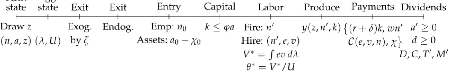
Drawz (n,a,z) Firm state Exog. byζ Exit Endog. Exit Emp:n0 Assets:a0−χ0 Entry k≤ ϕa Capital Fire:n′ Hire: (n′,e,v) V∗= ev dλ Labor θ∗ =V∗/U y(z,n′,k) Produce (r+δ)k,wn′ C(e,v,n),χ Payments a′ ≥0 d≥0 D,C,T′,M′ Dividends (λ,U) Agg. state
Figure 3: Timeline of the model
transform them into capital, and rent it to firms. The one-period contract with households pays a risk-free interest rate of r. Capital depreciates at rate δ in production, and so the price of
capital charged by banks to firms is(r+δ).
Households. We envision a representative household with ¯Lfamily members,U of which are
unemployed. The household is risk-neutral with discount factor β ∈ (0, 1). It trades shares M
of a mutual fund comprised of all firms in the economy and makes bank deposits T. It earns
interestr on deposits, the total wage payments that firms make to employed family members,
and Ddividends per share held in the mutual fund. Moreover, unemployed workers produce
ωunits of the final good at home. Household consumption is denoted byC.
Before describing the firm’s problem in detail, we outline the precise timing of the model, summarized in Figure 3. Within a period, the events unfold as follows: (i) realization of the productivity shocks for incumbent firms; (ii) endogenous and exogenous exit of incumbents; (iii) realization of initial productivity and entry decision of potential entrants; (iv) borrowing decisions by incumbents; (v) hiring/firing decisions and labor market matching; (vi) produc-tion and revenues from sales; (vii) payment of wage bill, costs of capital, hiring and operaproduc-tion expenses; firm dividend payment/saving decisions, and household consumption/saving deci-sions.
To be consistent with our transition dynamics experiments in Section5, it is useful to note that we record aggregate state variables—the measures of incumbent firms λand
unemploy-mentU—at the beginning of the period, between stages (i) and (ii). Moreover, even though the
labor market opens after firms exit or fire, workers who separate in the current period can only start searching in the next one.
3.2
Firm Problem
We first consider the entry and exit decisions, then analyze the problem of incumbent firms.
Entry. A potential entrant who has drawnzfromΓ0(z)solves the following problem
maxna0, Vi(n0,a0−χ0,z)
o
, (4)
where Vi is the value of an incumbent firm, a function of(n,a,z). The firm enters if the value
to the risk-neutral shareholder of becoming an incumbent with one employee (n0 =1), initial net worth equal to the household equity injectiona0 minus the entry costχ0, and productivity zexceeds the value of returninga0to the household. Leti(z) ∈ {0, 1}denote the entry decision rule, which depends only on the initial productivity draw, since all potential entrants share the same entry cost, initial employment and ex-ante equity injection. AsViis increasing inz, there
is an endogenous productivity cut-off z∗ such that for allz ≥z∗ the firm chooses to enter. The
measure of entrants is therefore
λe =λ0
Z
i(z)dΓ0 =λ0[1−Γ0(z∗)]. (5)
Exit. Firms exit exogenously with probabilityζ. Conditional on survival the firm then chooses
to continue or exit. An exiting firm pays out its net worthato shareholders. The firm’s expected
valueVbefore the destruction shock equals
V(n,a,z) =ζa+ (1−ζ)maxnVi(n,a,z), ao. (6)
We denote byx(n,a,z) ∈ {0, 1}the exit decision.
Hire or Fire. An incumbent firmi with employment, assets, and productivity equal to the
triplet(n,a,z)chooses whether to hire or fire workers to solve
Vi(n,a,z) =maxnVh(n,a,z),Vf(n,a,z)o. (7)
The two value functions Vf and Vh associated with firing (f) and hiring (h) are described
The Firing Firm. A firm that has chosen to fire some of its workers (or not to adjust its work force) solves Vf(n,a,z) = max n′,k,d d+β Z V(n′,a′,z′)Γ(dz′,z) (8) s.t. n′ ≤ n, d+a′ = y(n′,k,z) + (1+r)a−ωn′−(r+δ)k−χ, k ≤ ϕa, d ≥ 0.
Firms maximize shareholder value and, because of risk-neutrality, useβas their discount factor.
The change in net-worth a′−a is given by revenues from production and interest on savings
net of the wage bill, rental and operating costs, and dividend payoutsd. The last two equations
in (8) reiterate that firms face a collateral constraint on the maximum amount of capital they can rent and a non-negativity constraint on dividends.
To help understand the budget constraint and preface how we take the model to the data, define firm debt by the identityb ≡ k−a, with the understanding thatb < 0 denotes savings. Making this substitution reveals an alternative formulation of the model in which the firm owns its capital and faces a constraint on leverage. With state vector (n,k,b,z), the firm faces the following budget and collateral constraints
d+k′−(1−δ)k | {z } Investment = y(n′,k,z)−ωn′−χ−rb | {z } Operating Profit + b′−b | {z } ∆Borrowing , b/k ≤ (ϕ−1)/ϕ.
This makes clear that the firm can fund equity payouts and investment in capital through either operating profits or expanding borrowing/reducing saving.
The Hiring Firm. The hiring firm additionally chooses the number of vacancies to postv ∈R+
and recruitment effort e ∈ R+, understanding that, by a law of large numbers, its new hires n′−nequal the firm’s job-filling rateqeof each of its vacancies times the number of vacancies
vcreated: n′−n =q(θ∗)ev.6 Note that the individual job-filling rate depends on the aggregate
meeting rate q, which is determined in equilibrium and the firm takes as given, as well as its
recruiting efforte. The firm faces a variable cost functionC(e,v,n), increasing and convex ine
andv.
A firm’s continuation value depends on n′, not on the mix of recruiting intensity e and
vacant positions v that generates it. As a result, one can split the problem of the hiring firm
in two stages. First, the choice of n′, k and d. Second, given n′, the choice of the optimal
combination of inputs(e,v). The latter reduces to a static cost-minimization problem:
C∗ n,n′ =min
e,v C(e,v,n) (9)
s.t. e≥0, v≥0, n′−n=q(θ∗)ev.
yielding the lowest cost combination e(n,n′) and v(n,n′) that delivers h = n′−n hires to a
firm of sizen, and implied cost functionC∗(n,n′).
The remaining choices ofn′,kanddrequire solving the dynamic problem Vh(n,a,z) = max n′,k,d d+β Z V(n′,a′,z′)Γ(dz′,z) (10) s.t. n′ > n, d+a′ = y(n′,k,z) + (1+r)a−ωn′−(r+δ)k−χ− C∗ n,n′, k ≤ ϕa, d ≥ 0.
The solution of this problem includes the decision rule n′(n,a,z). Using this function in the solution of (9), we obtain decision rules e(n,a,z) and v(n,a,z) for recruitment effort and va-cancies in terms of firm state variables.
Given the centrality of the hiring cost functionC(e,v,n) to our analysis, we now discuss its
specification. In what follows, we choose the functional form C(e,v,n) = κ1 γ1e γ1+ κ2 γ2+1 v n γ2 v, (11)
with γ1≥1 andγ2 ≥0 being necessary conditions for convexity of the maximization problem (9). This cost function implies that the average cost of a vacancy, C/v, has two separate
com-ponents. The first is increasing and convex in recruiting intensity per vacancy e. The idea is
that, for any given open position, the firm can choose to spend resources on recruitment activi-ties (recall Figure2) to make the position more visible or the firm more attractive as a potential employer, or to assess more candidates per unit of time, but all such activities are increasingly costly on a per-vacancy basis. The second component is increasing and convex in the vacancy rate, and captures the fact that expanding productive capacity is costly in relative terms: for
example, creating 10 new positions involves a more expensive reorganization of production in a firm with 10 employees than in a firm with 1000 employees.
In AppendixAwe derive several results for the static hiring problem of the firm(9)under this cost function and derive the exact expression for C∗(n,n′) used in the dynamic problem (10). We show that, by combining first-order conditions, we obtain the optimal choice ofe
e n,n′ = κ2 κ1 γ1 γ1−1 γ 1 1+γ2 q(θ∗)− γ2 γ1+γ2 n′−n n γγ2 1+γ2 , (12)
and, hence, the firm-level job filling rate f (n,n′) ≡ q(θ∗)e(n,n′), as well as the optimal
vacancy-rate: v n = κ2 κ1 γ1 γ1−1 γ 1 1+γ2 q(θ∗)− γ1 γ1+γ2 n′−n n γγ1 1+γ2 . (13)
Equation (12) demonstrates that the model implies a log-linear relation between the job filling rate and employment growth at the firm level, with elasticity γ2/(γ1+γ2). This is the key empirical finding ofDFH, who estimate this elasticity to be 0.82. In fact, one could interpret our functional choice for C in equation(11) as a ‘reverse-engineering’ strategy in order to obtain, from first principles, the empirical cross-sectional relation between firm-level job-filling rate and firm-level hiring rate uncovered byDFH. Put differently, micro data sharply discipline the
Figure 4: Cross-sectional relationships between monthly employment growth (n′−n)/n and
the vacancy ratev/nand the job filling rateeq. Data fromDFHonline supplemental materials.
-0.3 -0.2 -0.1 0 0.1 0.2 Growth rate 0 0.01 0.02 0.03 0.04 0.05 0.06 V a ca n cy ra te A. Vacancy rate Model Data -0.3 -0.2 -0.1 0 0.1 0.2 Growth rate 0 1 2 3 4 5 6 7 8 J o b fi ll in g ra te
B. Jobfilling rate Model
Data
recruiting cost function of the model.7
Why does firm optimality imply that the job filling rate increases with the growth rate with elasticityγ2/(γ1+γ2)? Recruiting intensityeand the vacancy rate(v/n)are substitutes in the production of a target employment growth rate(n′−n)/n—see the last equation in (9). Thus,
a firm that wants to grow faster than another will optimally create more positions and, at the same time, spend more in recruiting effort. However, the stronger the convexity of C in the vacancy rate (γ2), relative to its degree of convexity in effort(γ1), the more an expanding firm finds it optimal to substitute away from vacancies into recruiting intensity to realize its target growth rate. In the special case whenγ2 = 0, all the adjustment occurs through vacancies and recruiting effort is irresponsive to the growth rate and to macroeconomic conditions, as in the canonical model ofPissarides(2000).
Figure 4 plots the cross-sectional relationship between the vacancy rate and employment growth (panel A) and the job filling rate and employment growth (panel B) in the model and in theDFHdata, with the elasticity of the job filling rate to firm’s growthγ2/(γ1+γ2) =0.82.8 Since the individual hiring function is linear in vacancies, the elasticity of the vacancy rate to
7AppendixAalso shows that, once the optimal choice ofeis substituted into(11),C can be stated solely in
terms of the vacancy rate and becomes equivalent to one of the hiring cost functions thatKaas and Kircher(2015) use in their empirical analysis.
8In Figure4, the model implies zero hires for firms with negative growth rates, whereas in the data time
firm’s growth equalsγ1/(γ1+γ2) = 0.18.
3.3
Household Problem
The representative household solves
W(T,M) = max
T′,M′,C>0 C+β
W(T′,M′) (14) s.t.
C+QT¯ ′+PM′ = ωL¯ + (D+P)M+T,
whereCdenotes household consumption;Tare bank deposits;Mare shares of the mutual fund
composed of all firms in the economy, with the aggregate number of shares normalized to one; ¯
Ldenotes the number of household members. The share price is Pand owning shares entitles
the household to dividends D, the sum of all firm dividends.9 Since the return from working
in the market and working at home are the same, total income is simply ωL¯ (which is also the
reason why unemploymentU is not a state variable in the household’s problem).
The total wage bill is the integral over all wage payments from firms, while workers that are idle this period and begin next period as unemployed job seekers produce ω units of the
final good via home production. Unemployment evolves due to masses of hires H(θ∗) and
separations of massF(θ∗), which the household takes as given and we characterize later. From the first-order conditions for deposits and share holdings, we obtain ¯Q = β and P =
β(P+D) which imply a constant return of r = β−1−1 on both deposits and shares and, thus, the household is indifferent over portfolios. Since the household is risk neutral, it is also indifferent over the timing of consumption.
3.4
Stationary Equilibrium and Aggregation
Let ΣN, ΣA, and ΣZ be the Borel sigma algebras over N and A, and Z. The state space for
an incumbent firm is S = N×A×Z, and we denote with s one of its points (n,a,z). Let ΣS be the sigma algebra on the state space, with typical set S =N × A × Z, and (S,ΣS) be
the corresponding measurable space. Denote with λ : ΣS → [0,∞) the stationary measure of
incumbent firms at the beginning of the period, following the draw of firm level productivity, before the exogenous exit shock.
To simplify the exposition of the equilibrium, it is convenient to use s ≡ (n,a,z) and s0 ≡ (n0,a0−χ0,z)as the argument for incumbents’ and entrants’ decision rules.
A stationary recursive competitive equilibrium is a collection of firms’ decision rules {i(z),x(s),n′(s),e(s),v(s),a′(s),d(s),k(s)}, value functionsV,Vi,Vf,Vh , a measure of
entrants λe, share price P and aggregate dividends D, wage ω, a distribution of firms λ, and
a value for effective labor-market tightness θ∗ such that: (i) the decision rules solve the firms
problems (4)-(10), V,Vi,Vf,Vh are the associated value functions, and λe is the mass of
entrants implied by (5); (ii) the market for shares clears atM =1 with share price
P = S V(s)dλ+λ0 Z i(z)Vi(s0)dΓ0
and aggregate dividends
D=ζ S adλ+ (1−ζ) S {[1−x(s)]d(s) +x(s)a}dλ−λ0 Z i(z)a0dΓ0; (iii) the stationary distribution λis the fixed point of the recursion:
λ(N × A × Z) = (1−ζ) S [1−x(s)]1{n′(s)∈N }1{a′(s)∈A}Γ(Z,z)dλ (15) +λ0 Z i(z)1{n′(s0)∈N }1{a′(s0)∈A}Γ(Z,z)dΓ0,
where the first term refers to existing incumbents and the second to new entrants; (iv) effective market tightnessθ∗ is determined by the balanced flow condition
¯
L−N(θ∗) = F(θ
∗)−λ
e(θ∗)n0
p(θ∗) , (16)
where p(θ∗)is the aggregate job finding rate,N(θ∗)is aggregate employment
N(θ∗) = (1−ζ) S [1−x(s)]n′(s)dλ+λ0 Z i(z)n′(s0)dΓ0, (17)
and F(θ∗)are aggregate separations F(θ∗) = ζ S ndλ+ (1−ζ) S x(s)ndλ+ (1−ζ) S [1−x(s)] n−n′(s)−dλ, (18)
which include all employment losses from firms exiting exogenously and endogenously, plus all the workers fired by shrinking firms, which we have denoted by (n−n′(s))−.10 In equa-tions(16)-(18), the dependence of λe, N and Fonθ∗ comes through the decision rules and the
stationary distribution, even though, for notational ease, we have omitted θ∗ as their explicit
argument.
The left-hand side of (16) is the definition of unemployment—labor force minus employment—whereas the right-hand side is the steady-state Beveridge curve, i.e., the law of motion for unemployment
U′ =U−p(θ∗)U+F(θ∗)−λe(θ∗)n0 (19)
evaluated in steady state. As in Elsby and Michaels(2013), the two sides of (16) are
indepen-dent equations determining the same variable—unemployment—and, combined, they yield equilibrium market tightness θ∗.11 Note that equations (16) and (19) account for the fact that
every new firm enters with n0 workers hired ‘outside’ the frictional labor market (e.g., the founders).
Clearly, once θ∗ and λ are determined, so isU from either side of (16) and, therefore, V∗.
Finally, we note that measured aggregate matching efficiency, in equilibrium, is Φ= (V∗/V)α,
where measured and effective vacancies are respectively
V = (1−ζ) S [1−x(s)]v(s)dλ +λ0 Z i(z)v(s0)dΓ0, V∗ = (1−ζ) S [1−x(s)]e(s)v(s)dλ+λ0 Z i(z)e(s0)v(s0)dΓ0.
10Entrant firms never fire, as they enter with the lowest value on the support forN,n 0.
11Our computation showed that, typically, N(θ∗)is decreasing in its argument and the right-hand side of(16) is always positive and decreasing. Thus, the crossing point of left- and right-hand side is unique, when it exists. However, an equilibrium may not exist. For example, for very low hiring costs, N(θ∗) may be greater than ¯L. Conversely, for large enough operating or hiring costs, no firms will enter the economy. In this case, there is no equilibrium with market production (albeit there is always some home-production in the economy).
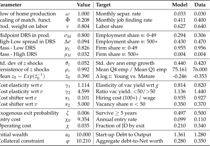
Table 1: Externally set parameter values
Parameter Value Target
Discount factor (monthly) β 0.9967 Annual risk-free rate = 4%
Mass of potential entrants λ0 0.02 Measure of incumbents = 1 Size of labor force L¯ 24.6 Average firm size = 23
Elasticity of matching function wrtVt α 0.5 JOLTS
AppendixCprovides details on the computation of the decision rules and the stationary equi-librium.
4
Parameterization
4.1
Externally Calibrated
We begin from the subset of parameters that are calibrated externally. The model period is one month. We set β to replicate an annualized risk-free rate of 4 percent. Since the measure of
potential entrantsλ0scalesλ—see equation(15)—we chooseλ0to normalize the total measure of incumbent firms to one. We normalize the size of the labor force ¯Lso that, given a measure
one of firms, under our target unemployment rate of 7 percent, the average firm size will be 23 consistent with Business Dynamics Statistics (BDS) data over the period 2001-2007.12 In line with empirical studies, we set α, the elasticity of aggregate hires to aggregate vacancies in the
matching function, to 0.5. Table1summarizes these parameter values.
4.2
Internally Calibrated
Table 2 lists the remaining 19 parameters of the model that are set by minimizing the dis-tance between an equal number of empirical moments and their equilibrium counterparts in the model.13 Table 2 lists the targeted moments, their empirical values, and their simulated
12The unemployment rate isu = L¯/N(θ∗)−1, and with a unit mass of firms the average firm size is simply
N(θ∗). Hence givenu=0.07, ¯Ldetermines average firm size.
13Specifically, the vector of parametersΨis chosen to minimize the minimum-distance-estimator criterion
func-tion
Table 2: Parameter values estimated internally
Parameter Value Target Model Data
Flow of home production ω 1.000 Monthly separ. rate 0.033 0.030
Scaling of match. funct. Φ¯ 0.208 Monthly job finding rate 0.411 0.400
Prod. weight on labor ν 0.804 Labor share 0.627 0.640
Midpoint DRS in prod. σM 0.800 Employment sharen: 0-49 0.294 0.306
High-Low spread in DRS ∆σ 0.094 Employment sharen: 500+ 0.430 0.470
Mass - Low DRS µL 0.826 Firm sharen: 0-49 0.955 0.956
Mass - High DRS µH 0.032 Firm sharen: 500+ 0.004 0.004
Std. dev ofzshocks ϑz 0.052 Std. dev ann emp growth 0.440 0.420
Persistence of zshocks ρz 0.992 Mean Q4 emp / Mean Q1 emp 75.161 76.000
Meanz0 ∼Exp(z¯−01) z¯0 0.390 ∆logz: Young vs. Mature -0.246 -0.353 Cost elasticity wrte γ1 1.114 Elasticity of vac yield wrtg 0.814 0.820 Cost elasticity wrtv γ2 4.599 Ratio vac yield: <50/>50 1.136 1.440 Cost shifter wrt e κ1 0.101 Hiring cost (100+) / wage 0.935 0.927 Cost shifter wrt v κ2 5.000 Vacancy sharen<50 0.350 0.370 Exogenous exit probability ζ 0.006 Survive≥5 years 0.497 0.500
Entry cost χ0 9.354 Annual entry rate 0.099 0.110
Operating cost χ 0.035 Fraction of JD by exit 0.210 0.340
Initial wealth a0 10.000 Start-up Debt to Output 1.361 1.280 Collateral constraint ϕ 10.210 Aggregate debt-to-Net worth 0.280 0.350
values from the model. Even though every targeted moment is determined simultaneously by all parameters, in what follows we discuss each of them in relation to the parameter for which, intuitively, that moment yields the most identification power.
We set the flow of home production of the unemployedω to replicate a monthly separation
rate of 0.03. We choose the shift parameter of the matching function (a normalization of the value of Φ in steady state) in order to pin down a monthly job finding rate of 0.40. Together,
these two moments yield a steady-state unemployment rate of 0.07.
We assume the revenue functiony(z,n′,k) =z(n′)νk1−νσand introduce a small degree of
permanent heterogeneity in the scale parameterσ.14 Specifically we consider a three-point dis-where mdata and mmodel(Ψ) are the vectors of moments in the data and model, and W = diag 1/m2data
is a diagonal weighting matrix.
14Since we specify therevenuefunction, we do not take a stand on whetherzrepresents demand or productivity
tribution with support{σL,σM,σH}—symmetric aboutσM—leaving four parameters to choose:
(i) the value of σM; (ii) the spread ∆σ ≡ (σH −σL); and (iii)-(iv) the fractions of low and high
DRS firms µL,µH. In the same spirit as the use of permanent heterogeneity in productivity in
the quantitative applications ofElsby and Michaels(2013) andKaas and Kircher(2015), hetero-geneity in the scale of production allows us to match the firm size distribution and to generate, within the model, small old firms alongside young large firms, thus decoupling age and size which tend to be too strongly correlated in standard firm dynamics models with stochastic pro-ductivity. In addition, the assumption of heterogeneity in σ captures the appealing idea that
there exist some very productive, but small, businesses simply because the optimal scale of production for many goods or services is small. The values of these four parameters allow the model to match the BDS statistics on employment and establishment shares of firms of size 0-49 and 500+.15
Firm productivity z follows an AR(1) process in logs: logz′ = logZ +ρzlogz+ε, with
ε ∼ N(−ϑz2/2,ϑz). We calibrate ρz andϑz to match two measures of employment dispersion,
one in growth and one in levels: the standard deviation of annual employment growth for continuing establishments in the Longitudinal Business Database (Elsby and Michaels, 2013), and the ratio of the mean size of fourth to first quartile of the firm distribution (Haltiwanger, 2011a).16
The initial productivity distribution for entrants Γ0 is Exponential, with mean ¯z0
cho-sen to match the productivity gap between entrants and incumbents, specifically the dif-ferential in revenue productivity between firms older than 10 and younger than 1 year old (Foster, Haltiwanger, and Syverson,2016).
We now turn to hiring costs. The cost function(11)has four parameters: the two elasticities (γ1,γ2) and the two cost shifters (κ1,κ2). Recall, from the discussion surrounding equations (11) and (12), that the cross-sectional elasticity of job filling rates to employment growth rates, estimated to be 0.82 by DFH, is a function of the ratio of these two elasticities.17 The second
sloping demand curve. Given this understanding we discuss the revenue function as if it were a production function: σ represents span of control andz is total factor productivity. Sedlacek and Sterk(2014) solve a firm
dynamics model where scale heterogeneity arises because different producers face demand curves with different elasticities.
15In terms of the description of the model and stationary equilibrium, one should addσto the firm’s state vector
s, but nothing substantial in the firm problem and the definition of equilibrium would change.
16In the numerical solution and simulation of the model,zremains a continuous state variable. 17
moment used to separately identify the two elasticities is the ratio of vacancy yields of small (< 50 employees) to large (> 50 employees) firms from JOLTS data on hires and vacancies by firm size. Intuitively, when γ2 = 0, recruiting effort is constant across firms and this ratio is one.
We use two targets to pin down the cost shift parameters. The first is the total hiring cost as a fraction of monthly wage per hire, a standard target for the single vacancy cost parameter that usually appears in vacancy posting models. We have a new source for this statistic. The con-sulting company Bersin and Associates runs a periodic survey of recruitment cost and practices based on over 400 firms—all with more than 100 employees. Once the firms are re-weighted by industry and size, the sample is representative of this size segment of the US economy. They compute that, on average, annual spending on all recruiting activities (including internal staff compensation, university recruiting, agencies/third-party recruiters, professional networking sites, job boards, social media, contractors, employment branding services, employee refer-ral bonuses, pay-per-click media, travel to interview candidates, applicant tracking systems, print/media/billboards, other tools/technologies) divided by the number of hires in 2011 was $3,479 (see Table 3 in O’Leonard 2011). Given average annual earnings of roughly $45,000 in 2011, in the model we target a ratio of average recruiting cost to average monthly wage (in firms with more than 100 employees) of 0.928. The second target is the vacancy share of small (n < 50) firms from JOLTS: κ2 determines the size of hiring costs for small (low n) firms and, thus, the amount of vacancies they create.
The parametersχandζ have large effects on firm exit. The operation costχmostly impacts
exit rates of young firms; therefore, we target the five-year survival rate found in BDS data, which is approximately 50 percent. The parameter ζ contributes to the exit of large and old
firms; hence we target the fraction of total job destruction due to exit. To pin down the set-up costχ0, we target the annual entry-rate of 11 percent from the BDS.18
The remaining two parameters are the size of the initial equity injectiona0and the collateral parameter ϕ. To inform their calibration, we target the debt-output ratio of start-up firms com-tency, the growth rate is the Davis-Haltiwanger growth rate normalized in[−2, 2]. In practice, as seen in Table2, the discrepancy between structural and estimated parameter is very small.
18When computing moments designed to be comparable to their counterparts in the BDS, we carefully
time-aggregate the model to an annual frequency. For example, the entry-rate in the BDS is measured as the number of age zero firms in a given year divided by the total number of firms. Computing this statistic in the model requires aggregating monthly entry and exit over 12 months. See AppendixCfor details.
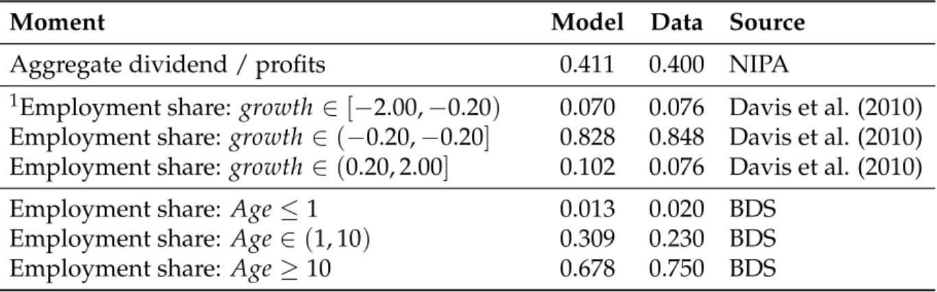
Table 3: Non-targeted moments
Moment Model Data Source
Aggregate dividend / profits 0.411 0.400 NIPA
1Employment share: growth ∈ [−2.00,−0.20) 0.070 0.076 Davis et al. (2010) Employment share:growth ∈ (−0.20,−0.20] 0.828 0.848 Davis et al. (2010) Employment share:growth ∈ (0.20, 2.00] 0.102 0.076 Davis et al. (2010) Employment share: Age ≤1 0.013 0.020 BDS
Employment share: Age ∈(1, 10) 0.309 0.230 BDS Employment share: Age ≥10 0.678 0.750 BDS
(1.) Firm growth rates are annual and are interior to[−2, 2]so do not include entering and exiting firms
puted from the Kauffman Survey (Robb and Robinson, 2014), and the aggregate debt to total assets ratio from the Flow of Funds.19
4.3
Cross-Sectional Implications
We now explore the main cross-sectional implications of the calibrated model, at its steady-state equilibrium.
Table3reports some empirical moments that we did not target in the calibration and their model-generated counterparts. The fact that the ratio of dividend payments to profits in the model is close to its empirical value reinforces the view that our collateral constraint is neither too tight nor too loose. The model can also replicate well the distribution of employment by growth rate and by firm age, neither of which was explicitly targeted.
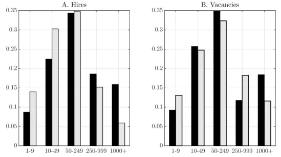
Figure5shows that the model is also able to replicate satisfactorily the observed distribution of hires and vacancies by size class from the JOLTS data.
In Figure 6 we plot the average firm size, job creation and destruction rates, fraction of constrained firms and leverage (debt/saving over net worth,b/a) for firms from birth through
19Robb and Robinson(2014) report $68,000 of average debt (credit cards, personal and business bank loans, and
credit lines) and $53,000 of average revenue for the 2004 cohort of start-ups in their first year, see their Table 5. From the Flow of Funds 2005, we computed total debt as the sum of securities and loans and total assets as the sum of all nonfinancial assets plus financial assets net of trade receivables, FDIs and miscellaneous liabilities (Tables L.103 and L.104, Liabilities of Nonfinancial Corporate and Noncorporate Business), and divided by the sum of corporate and noncorporate net worth (Tables B.103 and B.104, Balance Sheet of Nonfinancial Corporate and Noncorporate Business).
Figure 5: Hire and vacancy shares by size class. Model in blue, JOLTS data 2002-2007 in red. 1-9 10-49 50-249 250-999 1000+ 0 0.05 0.1 0.15 0.2 0.25 0.3 0.35 A. Hires 1-9 10-49 50-249 250-999 1000+ 0 0.05 0.1 0.15 0.2 0.25 0.3 0.35 B. Vacancies
to maturity. Panel A shows that σH-firms, those with closer to constant returns in production,
account for the upper tail in the size and growth-rate distributions. On average, though, firm size grows by much less over the life cycle, since these ‘gazelles’—as they are often referred to in the literature—are only a small fraction of the total. On average, the model and the data line up well: average size grows by a factor of 3 between ages 1-5 and 20-25 in the model and 3.4 in the BDS data. Convex recruiting costs and collateral constraints slow down growth: most firms reach their optimal size around age 10, andσH-firms keep growing for much longer.
Panel B plots job creation and destruction rates by age. It is a stark representation of the ‘up-or-out’ dynamics of young firms documented in the literature (Haltiwanger,2011b). Panel C depicts the fraction of constrained firms (defined as those with k = ϕa and d = 0) over
the life cycle. In the model, financial constraints bind only for the first few years of a firm’s life, when net worth is insufficient to fund the optimal level of capital. Panel D illustrates that leverage declines with age and after age 10 the median firm is saving (i.e.,b <0). Much like in the classical household ‘income fluctuation problem,’ in our model firms have a precautionary saving motive due to the simultaneous presence of three elements: (i) a concave payoff function because of DRS; (ii) stochastic productivity; and (iii) the collateral constraint.
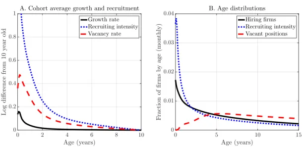
Panel A of Figure7shows that recruiting intensity and the vacancy rate are sharply decreas-ing with age. These features arise because our cost function implies that both optimal hirdecreas-ing effort and optimal vacancy rates are increasing in the growth rate, and young firms are those
Figure 6: Average life cycle of firms in the model 0 1 2 3 4 5 Age (years) 0 0.05 0.10 0.15 0.20
0.25 B. Job creation and destruction
Job creation rate Job destruction rate
0 5 10 15 Age (years) 0 100 200 300 400 A. Average size HighσH MedσM LowσL 0 1 2 3 4 5 Age (years) 0 0.2 0.4 0.6 0.8 1 C. Fraction offirms constrained 0 5 10 15 20 Age (years) 0 5 10 15 D. Average leverage
with the highest desired growth rates. Moreover, the stronger convexity of C in the vacancy rate (γ2), relative to its degree of convexity in effort(γ1)implies that a rapidly expanding firm prefers to substitute away from vacancies into recruiting intensity to realize its target growth rate. Thus, young firms find it optimal to limit the number of new positions, but recruit very aggressively for the ones that they open. As firms age, growth rates fall and this force weakens. Panel B plots the fraction of total recruiting effort, vacancies and hiring firms by age. It shows that, relative to the steady-state age distribution of hiring firms, the effort distribution is skewed towards young firms, whereas the vacancy distribution is skewed towards older firms. In the model the age-distribution of vacancies is almost uniform: young firms grow faster than old ones and, thus, post more vacancies per worker; however, they are smaller and, thus, they post fewer vacancies for a given growth rate. These two forces counteract each other and the ensuing vacancy distribution over ages is nearly flat. Figure7highlights that the JOLTS notion of vacancy as ‘open position ready to be filled’ is a good metric of hiring effort for old firms, for whom recruiting intensity is nearly constant, whereas it is quite imperfect for young firms aged 0-5, whose average recruiting intensity, as well as its variance, are much higher than those
Figure 7: Vacancy and Effort Distributions by Age 0 2 4 6 8 10 Age (years) 0 0.2 0.4 0.6 0.8 1 L o g d i ff er en ce fr o m 1 0 y ea r o ld
A. Cohort average growth and recruitment Growth rate Recruiting intensity Vacancy rate 0 5 10 15 Age (years) 0 0.01 0.02 0.03 0.04 F ra ct io n o f fi rm s b y a g e (m o n th ly ) B. Age distributions Hiringfirms Recruiting intensity Vacant positions of mature firms.20
5
Aggregate Recruiting Intensity and Macroeconomic Shocks
Our main experiments examine the equilibrium of the economy along perfect foresight paths for shocks to aggregate productivity Zand to the financial constraint parameter ϕ. AppendixCprovides details on the solution of the model along these transitional dynamics away from, and back to, the steady state.
We frame these experiments in the context of the Great Recession. Specifically, we consider mean-reverting AR(1) shocks, choosing their size so that the model matches the maximum devi-ation of detrended output over 2008-2012 from its value in 2007, a value of -10 percent (Fernald, 2015). Their persistence is set so that the half-life of output dynamics is three years under both shocks. This strategy results in a 4-percent shock toZ, and a 75-percent shock toϕ.21
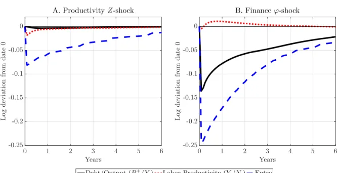
Figure8plots the dynamics of some key aggregate variables. The financial shock displays three features that are absent from the macroeconomic transition under the productivity shock, but present in the data. First, a sizable drop in the debt-output ratio of magnitude and
persis-20Unfortunately, the JOLTS does not report the age of the firm, so there are no U.S. data on vacancies and
recruiting intensity by firm age we can directly compare to our model.Kettemann, Mueller, and Zweimuller(2016) find that, in Austrian data, after controlling for firm fixed effects job filling rates are decreasing with firm age.
21The implied (monthly) persistence parameters are 0.990 forZand 0.976 forϕ. FigureB1in AppendixB
Figure 8: Dynamics of some macroeconomic variables 0 1 2 3 4 5 6 Years -0.25 -0.2 -0.15 -0.1 -0.05 0 L o g d ev ia ti o n fr o m d a te 0 A. Productivity Z-shock 0 1 2 3 4 5 6 Years -0.25 -0.2 -0.15 -0.1 -0.05 0 L o g d ev ia ti o n fr o m d a te 0 B. Finance ϕ-shock Debt/Output (B+
t /Yt) Labor Productivity (Yt/Nt) Entry
tence comparable to the data.22 Second, an endogenousrisein aggregate labor productivity of
1.5 percent, close to the 2 percent rise over 2008-10 measured byMcGrattan and Prescott(2012). Labor productivity rises because more severe financial frictions prevent the expansion of firms, especially the high-σones with large scale of production, as we will show more in detail below.
As firm size falls, because of DRS, average labor productivity increases. Third, a 24 percent de-cline in entry which, again, matches well its empirical counterpart of 22 percent.23 Specifically, young-firm values decline sharply, since a large fraction of them are constrained (recall Figure
6), leading to a decline in start-ups. Overall, we conclude that the differential responses of these three variables clearly identify a financial shock in the 2008 recession.
Figure 9 displays the dynamics of the key labor market variables under the two shocks. Overall, in both experiments the labor-market response to the shock is close to its empirical counterpart of Figure1.24 The financial shock induces bigger and more persistent movements in vacancies, unemployment, and the job finding rate. Under both scenarios, the drop in aggregate recruiting intensity is sizable, but its magnitude and persistence are, again, larger under the
22In the US since 2008, the debt-output ratio drops by nearly 10 percent points and five years later is still 4
percent below its pre-recession level.
23Entry in the data is measured as the number of firms reporting an age of zero divided by the total number of
firms in the LBD. The survey is in March and so this measure excludes firms which enter and exit between surveys.
24In the data, labor market variables move more slowly, but recall that the shocks we fed are AR(1) designed to
Figure 9: Dynamics of labor market variables 0 1 2 3 4 5 6 Years -1 -0.5 0 0.5 1 L o g d ev ia ti o n fr o m d a te 0 A. ProductivityZ-shock 0 1 2 3 4 5 6 Years -1 -0.5 0 0.5 1 L o g d ev ia ti o n fr o m d a te 0 B. Financeϕ-shock
Vacancies Vacancy yield Unemployment Jobfinding rate Agg. recruiting intensity
financial shock: Φt falls by 25 percent at impact (20 percent under the productivity shock) and
five years later it is still 10 percent below its initial value (5 percent under the productivity shock).25 We conclude that, in the model, the financial shock—the more promising candidate to rationalize the Great Recession based on our discussion of Figure8—can explain around half of the observed decline in aggregate match efficiency (recall the empirical path in Figure1).
At first sight, it may be surprising that the response of aggregate recruiting intensity is not too dissimilar across the two macro shocks although the entry rate of new firms—which ac-counts for a disproportionate share of job creation—remarkably differs under the two experi-ments. In what follows, we explain this apparent puzzle.
5.1
The Transmission Mechanism
To understand how macro shocks transmit to aggregate recruiting intensity, we return to our expression forΦt, usingλhto denote the distribution of hiring firms:
Φt = Vt∗ Vt α = eit vit Vt dλht α . (20)
25We note that the persistence ofΦ
tis higher under the financial tightening in spite of the fact that the financial shock itself is less persistent than the productivity shock.
Substituting the policy function for recruitment effort (12) i