Research Article
A Modified Priority-Based Encoding for Design of
a Closed-Loop Supply Chain Network Using a Discrete
League Championship Algorithm
Javid Ghahremani Nahr,
1Ramez Kian
,
2,3and Hassan Rezazadeh
3 1Academic Center for Education, Culture and Research (ACECR), Tabriz, Iran2Nottingham Business School, Nottingham Trent University, UK 3Department of Industrial Engineering, University of Tabriz, Tabriz, Iran Correspondence should be addressed to Ramez Kian; [email protected]
Received 6 January 2018; Accepted 11 April 2018; Published 17 May 2018
Academic Editor: Guillermo Cabrera-Guerrero
Copyright © 2018 Javid Ghahremani Nahr et al. This is an open access article distributed under the Creative Commons Attribution License, which permits unrestricted use, distribution, and reproduction in any medium, provided the original work is properly cited.
In a closed-loop supply chain network, the aim is to ensure a smooth flow of materials and attaining the maximum value from returning and end-of-life goods. This paper presents a single-objective deterministic mixed integer linear programming (MILP) model for the closed-loop supply chain (CLSC) network design problem consisting of plants, collection centers, disposal centers, and customer zones. Our model minimizes the total costs comprising fixed opening cost of plants, collection, disposal centers, and transportation costs of products among the nodes. As supply chain network design problems belong to the class of NP-hard problems, a novel league championship algorithm (LCA) with a modified priority-based encoding is applied to find a near-optimal solution. New operators are defined for the LCA to search the discrete space. Numerical comparison of our proposed encoding with the existing approaches in the literature is indicative of the high quality performance of the proposed encoding.
1. Introduction
Nowadays, supply chain management (SCM) has received attention in several organizations. SCM is described as the design, production, organization, execution, control, and testing regarding supply chain activities with the goal of creating net value, minimizing the logistics cost, creating a competitive infrastructure, synchronizing demand with supply, leveraging worldwide supply chain, and measuring effectiveness globally. Generally, SCM includes the coordi-nation and integration of key business activities including activities from purchase of raw materials to distribution of the finished products to customers. An efficient and effective supply chain can be regarded as a competitive advantage for companies and plants and helps them to cope with the global market pressure. There are two kinds of supply chain, i.e., forward supply chains and reverse supply chains. The forward supply chain is defined as a set of activities converting raw materials to products as well as storing and distributing
products to the customers, while the reverse supply chain consists of a series of activities such as collection, inspection, repair, recovery, and disposal of used products. Integration of reverse and forward supply chains creates a CLSC. In other words, both forward and reverse supply chain networks are present in the CLSC networks. Network design is one of the most significant strategic decisions in SCM. In general, supply chain network design decisions include determining the number and location of facilities and the quantity of flow between them. In recent years, a few studies have focused on integrated forward and reverse network designs, while this type of integration can prevent the suboptimality and increase the level of network performance and coordination between forward and reverse processes. The present paper proposes a MILP model for design of a CLSC network consisting of plants, collection centers, disposal centers, and customer zones. Furthermore, it addresses two different problems, i.e., the facility location problem and the quantity of flow between facility optimization. A discrete LCA with a
Volume 2018, Article ID 8163927, 16 pages https://doi.org/10.1155/2018/8163927
new modified priority-based encoding is applied to solve the proposed model to minimize the total network costs.
2. Literature Review
Over recent years, considering the rising importance of reverse and CLSC network designs, numerous articles have been published in this regard. Govindan et al. [1] present a more comprehensive literature review regarding the closed-loop and reverse supply chains. They classify 382 papers published from 2007 to 2013 and propose a more detailed classification based on 10 factors, e.g., the year of release, approaches, objectives, and functions. They assert that almost 50% of the total surveys are linked to the CLSC network design, and almost 40% of them are connected to the reverse supply chain network design (RSCND). Furthermore, the mentioned study reveals that 12% and 88% of the published papers are related to the single-objective and multiobjective models, respectively. Most of the logistics network (RL) design problems (both forward and reverse logistics) include different MILP-based facility location models. These models include vast varieties from simple ones, such as locating facilities with unlimited capacity and lightweight single-piece model, and single product (e.g., [2]) to more complex ones, such as models for limited-capacity multilevel or multiproduct and multiperiod models (e.g., [3]). Jayaraman et al. [4] develop a MILP model for RL network design under a pull system based on customer demand for recycled products aiming to minimize the total cost. Krikke et al. [5] present a MILP for a two-stage RL network of a copier production plant. In their model, both processing returns and inventory costs are considered in the objective function. The uncertainty of the return number and quality of products is an important factor in the design of the RL network. Accordingly, Listes¸ and Dekker [6] present a MILP model for a sand recycling network with the aim of maximizing the total profit. They extend their model to the different conditions under several scenarios. Aras et al. [7] present a nonlinear model to determine the location of collection centers in a simple RL network. The most important thing to note in their paper is the ability of the proposed model in determining optimal purchase price of the used products with the profit-maximizing objective function. In their solution approach, they develop a heuristic method based on Tabu Search (TS) algorithm. ¨Uster et al. [8] develop a semi-integrated network in which there is a forward logistics network where only collection and recycling centers should be located. It optimizes forward and reverse flows simultaneously. They propose an exact approach based on Benders decomposition technique to solve the model. Lu and Bostel [9] consider a two-level location problem with three types of facilities that should be in a special reverse logistics called Reconstruction Location Network. They present a mixed integer binary programming model in which the forward and reverse flow and the interaction between them are considered at the same time. They also develop an algorithm based on Lagrangian heuristic algorithms to solve the model. Wojanowski et al. [10] study the interactions between industries and government agencies in relation to a series of products used by families.
In order to design a CLSC for third-party logistics providers Du and Evans [3] propose an advanced biobjective MILP model. The objective functions of their model are minimizing the lateness and the total cost. They develop a hybrid scatter search method to solve their model. Pishvaee et al. [11] propose a linear model for the location of collection and inspection centers in a reverse logistics network and develop a simulated annealing (SA) algorithm to solve the model in large-scale sizes. Bing et al. [12] consider the plastic recycling in the Netherlands. They propose a MILP model and aim to minimize transportation costs and environmental impacts under different scenarios to find the optimal separation strategy. Gomes et al. [13] propose a MILP model to find the optimal location for the collection and sorting centers. Selec-tion is carried out simultaneously under what called “Tactical Network Planning.” Their work is inspired by the European Union directive for electrical and electronic waste. Alumur et al. [14] propose a general MILP model with great flexibility that can be used for different recycled products and can be expanded further to include more settings. Their model determine optimal locations and capacities of inspection centers and reproduction plants in the design of RL network. Also, a case study with a RL network design concept for washing machines and dryers (large appliances) was studied in Germany. Their important assumption is that all the components of a product can be used again. Kannan et al. [15] propose a multistage, multiperiod, multiproduct integrated forward/reverse logistics network model for returned prod-ucts, which is based on GA-based heuristic algorithm. Listes¸ and Dekker [6] present a MILP model and certain dynamic aspects such as due dates and inventory status which results in a complicated model and for this reason they consider a single level single product network and solved it by genetic algorithms. Giri and Sharma [16] solve the problem with developed algorithms for sequential and global optimization. Pati et al. [17] perform a different formulation by presenting a MILP model for a better management of recycled paper logis-tics system. The authors examine the relationship between multiple targets of recycled paper distribution network such as RL costs, improving product quality and benefits of recycling waste-paper. In addition, their model determines strategic decisions such as locating facilities, as well as tactical decisions, such as recyclable product flows and routing under multi-item, multilevel, and multifacility. Godichaud and Amodeo [18] perform a multiobjective optimization in order to increase control policies with regard to returned products. Fonseca et al. [19] consider uncertainty with the cost of transportation and the waste of production. They present a comprehensive model for reverse logistics planning that consider levels of multiple facilities, multiple products, and selection of different technologies apart from being random. They present a two-stage biobjective mixed integer stochastic programming model for providing strategic and tactical decisions, respectively, in the first and second stages to minimize costs and also the negative impact. ¨Ozceylan et al. [20] develop a mixed integer nonlinear programming (MINLP) model, which optimizes the tactical decisions on balancing the decomposition lines in the reverse supply chain and the strategic decisions related to the quantity of
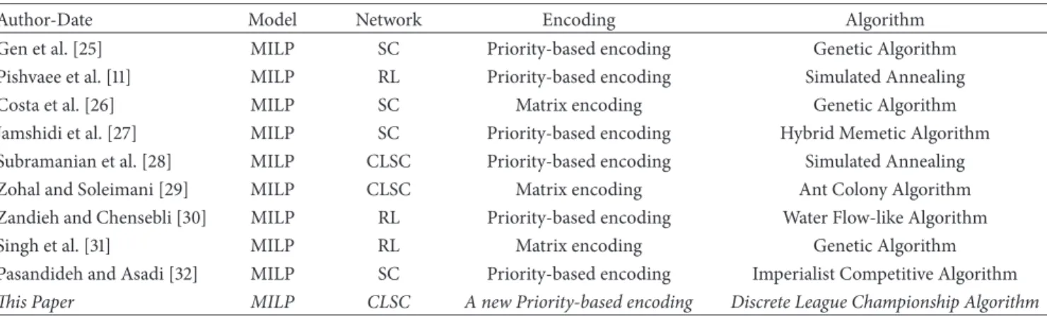
Table 1: Papers published in the field of SCND using metaheuristics algorithms.
Author-Date Model Network Encoding Algorithm
Gen et al. [25] MILP SC Priority-based encoding Genetic Algorithm
Pishvaee et al. [11] MILP RL Priority-based encoding Simulated Annealing
Costa et al. [26] MILP SC Matrix encoding Genetic Algorithm
Jamshidi et al. [27] MILP SC Priority-based encoding Hybrid Memetic Algorithm Subramanian et al. [28] MILP CLSC Priority-based encoding Simulated Annealing
Zohal and Soleimani [29] MILP CLSC Matrix encoding Ant Colony Algorithm
Zandieh and Chensebli [30] MILP RL Priority-based encoding Water Flow-like Algorithm
Singh et al. [31] MILP RL Matrix encoding Genetic Algorithm
Pasandideh and Asadi [32] MILP SC Priority-based encoding Imperialist Competitive Algorithm This Paper MILP CLSC A new Priority-based encoding Discrete League Championship Algorithm
products flowing on the CLSC. Soleimani et al. [21] propose a stochastic integer linear programming model for designing a multiproduct CLSC in the case of uncertainties regarding the demand, purchase price, and rate of return. Some of the most crucial studies addressing the supply chain are based on a metaheuristic algorithm (Table 1). However, recently other researchers have investigated this problem meticulously (e.g., [22, 23]). Table 1 summarizes similar works and highlights our contribution in this study.
3. Contribution Highlights
We contribute to the literature in three dimensions: (i) to the best of our knowledge, this work is the first League Champion Algorithm in which continuous encoded solu-tions are converted to discrete encoded solusolu-tions based on the new operators defined in this paper. (ii) We propose an efficient encoding methodology in our algorithm which keeps the generated solutions in the feasible region which causes speeding up of the algorithm and rising the chance of finding optimal solution. (iii) The numerical experiments demonstrate that our algorithm outperform similar existing ones in the literature and capable of solving large-scale problems in reasonable execution time which are not solvable via the commercial solver in reasonable time.
4. Problem Definition and Modeling
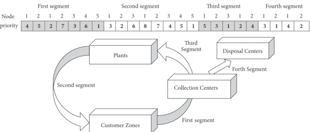
In the current study, a general CLSC network is considered. The forward network includes plants and customer zones, and the reverse network includes collection and disposal cen-ters. According to Figure 1, the plants could manufacture new products and remanufacture the returned ones. The plants send products to the customer zones. Then, the returned products from customers are collected by the collection centers, and after inspection of products, the repairable products are sent to the plants and the remaining ones are sent to the disposal center. To determine the scope of the study, the following assumptions are made for the proposed model.
(i) The model is designed for a single period. (ii) All facilities have limited and identified capacities.
Plants Customer Zones Disposal Centre Collection Centres Forward Supply Chain Reverse Supply Chain
Figure 1: The closed-loop supply chain network Amin and Zhang [24].
(iii) The locations of all centers are potential and un-known.
(iv) All customers demands must be satisfied and all the returned products from customers must be collected. (v) Customers locations are fixed and predefined. Given the above assumptions, the most important issue mentioned in this paper is locating the plants, collection centers, and disposal centers as well as determining the optimal amount of flow between centers. The network can be formulated as a MILP model. Sets, parameters, and decision variables are defined as follows:
Sets
𝐼: set of potential plants, whose elements are addressed by index𝑖 ∈ 𝐼
𝐽: set of fixed locations of customer zones, whose elements are addressed by index𝑗 ∈ 𝐽
𝐾: set of potential collection centers, whose elements are addressed by index𝑘 ∈ 𝐾
𝐿: set of potential disposal centers, whose elements are addressed by index𝑙 ∈ 𝐿
Parameters
TPS𝑖𝑗: unit transportation cost between plant𝑖 and customer zone𝑗
TSC𝑗𝑘: unit transportation cost between customer zone𝑗and collection center𝑘
TCP𝑘𝑖: unit transportation cost between collection center𝑘and plant𝑖
TCD𝑘𝑙: unit transportation cost between collection center𝑘and disposal center𝑙
𝐸𝑖: fixed cost for opening plant𝑖
𝐹𝑘: fixed cost for opening collection center𝑘
𝐺𝑙: fixed cost for opening disposal center𝑙 Cap𝑃𝑖: capacity of plant𝑖
Cap𝐶𝑘: capacity of collection center𝑘 Cap𝐷𝑙: capacity of disposal center𝑙 Dem𝑗: demand of customer𝑗
𝑟𝑗: return of customer𝑗
𝛽: minimum disposal fraction
Decision Variables
𝑋𝑖𝑗: quantity of new products shipped from plant𝑖to customer zone𝑗
𝑌𝑗𝑘: quantity of returned products from customer𝑗to
collection center𝑘
𝑆𝑘𝑖: quantity of returned products from collection center𝑘to plant𝑖
𝑇𝑘𝑙: quantity of returned products from collection center𝑘to disposal center𝑙
𝑍𝑖: 1, if a plant is located and set up at potential site𝑖, and0, otherwise
𝑊𝑘: 1, if a collection center is located and set up at potential site𝑘, and 0, otherwise
𝐻𝑙: 1, if a disposal center is located and set up at potential site l, and 0, otherwise.
4.1. Model Formulation. The mathematical model of the problem can be presented as follows:
Minimize: ∑ 𝑖 𝐸𝑖𝑍𝑖+ ∑ 𝑘 𝐹𝑘𝑊𝑘+ ∑ 𝑙 𝐺𝑙𝐻𝑙 + ∑ 𝑖 ∑ 𝑗 TPS𝑖𝑗𝑋𝑖𝑗+ ∑ 𝑗 ∑ 𝑘 TSC𝑗𝑘𝑌𝑗𝑘 + ∑ 𝑘 ∑ 𝑖 TCP𝑘𝑖𝑆𝑘𝑖+ ∑ 𝑘 ∑ 𝑙 TCD𝑘𝑙𝑇𝑘𝑙, (1) s.t. ∑ 𝑖 𝑋𝑖𝑗≥Dem𝑗, ∀𝑗 ∈ 𝐽, (2) ∑ 𝑖 𝑋𝑖𝑗≥ ∑ 𝑘 𝑌𝑗𝑘, ∀𝑗 ∈ 𝐽, (3) ∑ 𝑘 𝑌𝑗𝑘= 𝑟𝑗, ∀𝑗 ∈ 𝐽, (4) 𝛽∑ 𝑗 𝑌𝑗𝑘= ∑ 𝑙 𝑇𝑘𝑙, ∀𝑘 ∈ 𝐾, (5) ∑ 𝑗 𝑌𝑗𝑘= ∑ 𝑖 𝑆𝑘𝑖+ ∑ 𝑙 𝑇𝑘𝑙, ∀𝑘 ∈ 𝐾, (6) ∑ 𝑗 𝑋𝑖𝑗+ ∑ 𝑘 𝑆𝑘𝑖≤ 𝑍𝑖Cap𝑖𝑖, ∀𝑖 ∈ 𝐼, (7) ∑ 𝑗 𝑌𝑗𝑘≤ 𝑊𝑘Cap𝐶𝑘, ∀𝑘 ∈ 𝐾, (8) ∑ 𝑘 𝑇𝑘𝑙≤ 𝐻𝑙Cap𝐷𝑙, ∀𝑙 ∈ 𝐿, (9) 𝑍𝑖, 𝑊𝑘, 𝐻𝑙∈ {0, 1} , ∀𝑖 ∈ 𝐼, 𝑘 ∈ 𝐾, 𝑙 ∈ 𝐿, (10) 𝑋𝑖𝑗, 𝑌𝑗𝑘, 𝑆𝑘𝑖, 𝑇𝑘𝑙≥ 0, ∀𝑖 ∈ 𝐼, 𝑗 ∈ 𝐽, 𝑘 ∈ 𝐾, 𝑙 ∈ 𝐿. (11)
The first term in the objective function (1) represents the fixed costs of locating the plants. The second and third terms indicate the fixed costs of locating the collection centers and disposal centers, respectively. The fourth term corresponds to the production and transportation costs of new products. The fifth term represents the collection processing and transportation costs of returned products from customers. The sixth term calculates the recovery processing and trans-portation costs of returned products from collection centers to plants. The seventh term calculates the disposal processing and transportation costs of returned products from collection centers to disposal centers. Constraint (2) ensures that all customers demands are satisfied. Constraint (3) guarantees that forward flow is greater than reverse one. Constraint (4) computes the returned products from each customer. Constraint (5) enforces a minimum disposal fraction for each product. Constraint (6) indicates that the quantity of returned products from customer zones to collection centers is equal to the quantity of returned products from collection centers to plants and quantity of returned products from collection centers to disposal centers. Constraint (7) is a capacity constraint of plants. Constraint (8) is a capacity constraint for collection centers. Constraint (9) is a capacity constraint of disposal centers. Constraint (10) and (11) enforce the nonneg-ativity and binary restrictions on decision variables. The NP-hardness of supply chain network design problem has been proved by many research studies (e.g., [4]). The considered model in this paper consists of two different problems, i.e., facility location problem and quantity of flow between facility optimization; therefore, the developed model is reducible
First segment Second segment Third segment Fourth segment
Node 1 2 1 2 3 4 5 1 2 3 1 2 3 4 5 1 2 3 1 2 1 2 1 2
priority 4 5 2 7 3 6 1 3 2 6 8 7 4 5 1 5 3 1 2 4 3 1 4 2
Second segment
Plants Disposal Centers
Customer Zones First segment
Third Segment
Forth Segment
Collection Centers
Figure 2: An illustration of the CLSC network and its representation.
to facility location problem. Davis and Ray [33] concluded that facility location problem is NP-complete. Hence, the discussed CLSC network design problem is considered as NP-Hard in this paper. Solving this problem by exact solutions is time-consuming and sometimes impractical in large scales. Therefore, several metaheuristic algorithms with different approaches have been developed to get near optimal solu-tions, though all are not efficient. In the this paper, a discrete LCA solution approach is proposed and applied based on modified priority-based encoding.
5. Solution Approach
In this section, we first discuss about the encoded solution format which is referred to as “representation” in the rest of this manuscript and describe the discrete LCA used for solving the CLSC network design problem will be explained. 5.1. Representation. Representation is one of the most essen-tial issues for encoding and decoding, which affects the performance of algorithms. Tree-based representation is one way for representing network problems. There are several ways to encode the tree; for example, Gen and Cheng [34] introduce three ways of encoding the tree, i.e., edge-based encoding, vertex-based encoding, and edge-vertex encoding. Michalewicz et al. [35] use matrix-encoding representation, which belongs to edge-based encoding for solving the trans-portation tree. They present solutions through a |𝐾| × |𝐽| matrix in their approach, where|𝐾|and|𝐽|are the number of sources and depots, respectively. This method requires a large memory space on the computer. Another representation of transportation tree belonging to the vertex-based encoding is the Pr ¨Ufer number, which is developed by Gen and Cheng [34] wherein the solution is presented through|𝐾| + |𝐽| −
2 digits. Their method needs some repair mechanisms to obtain a feasible solution. Gen and Cheng [34] develop a priority-based encoding for solving the transportation tree, which does not need any excessive repair mechanisms and the solution is presented through|𝐾| + |𝐽|digits. Moreover,
this representation is applied to the shortest path problem and projects the scheduling problem. In the present paper, a modified priority-based encoding representation of Gen and Cheng [34] is proposed. In contrast to the other developed representations, presented in the literature, the suggested representation can solve the facility location and quantity flow optimization problems together. The representation includes four segments of sizes|𝐾| + |𝐽|,|𝐼| + |𝐽|,|𝐼| + |𝐾|, and
|𝐾|+|𝐿|digits, respectively, wherein the position of each digit represents the sources and depots within the supply chain network.
The first segment is devoted to the customers and collec-tion centers, the second segment is devoted to the plants and customers, the third segment is dedicated to the collection centers and plants, and finally the fourth segment is related to the collection and disposal centers. For example, the CLSC network depicted in Figure 2 includes five customers, two collection centers, three plants, and two disposal centers with the corresponding representations.
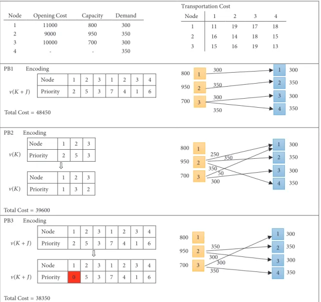
To demonstrate the effectiveness of the proposed rep-resentation in solving the supply chain problem, Figure 3 depicts the difference between the priority-based encoding developed by Gen et al. [25], priority-based encoding mod-ified by Jamshidi et al. [27], and priority-based encoding proposed in this paper, which are denoted by (PB1), (PB2), and (PB3), respectively. This figure illustrates a two-level supply chain with 3 sources and 4 depots, their corresponding capacities, depots demand, the opening cost of sources, transportation cost between the nodes, and the priority-based encoding. In the proposed representation, the solution is presented through|𝐾| + |𝐽|digits, where the position of each digit represents the sources and depots within the supply chain network. Furthermore, the value in digits denotes the priorities. After the encoding operation, in order to create a connection between the representation and the supply chain network, the decoding should be performed in a specific manner in which the output denotes the facilities opened and transportation amount between opened centers, as well. To decode the representation, first the potential facilities is
Node Opening Cost Capacity Demand 1 11000 800 300 2 9000 950 350 3 10000 700 300 4 350 Transportation Cost Node 1 2 3 4 1 11 19 17 18 2 16 14 18 15 3 15 16 19 13 Encoding PB1 - -Node 1 2 3 1 2 3 4 Priority 2 5 3 7 4 1 6 Encoding PB2 Node 1 2 3 Priority 2 5 3 Node 1 2 3 Priority 1 3 2 Encoding PB3 Node 1 2 3 1 2 3 4 Priority 2 5 3 7 4 1 6 Node 1 2 3 1 2 3 4 Priority 0 5 3 7 4 1 6 1 2 3 1 2 3 4 800 950 700 300 350 300 350 300 350 300 350 50 1 2 3 1 2 3 800 950 700 4 300 350 300 350 250 350 300 350 300 1 2 3 1 2 800 950 700 3 4 300 350 300 350 350 350 300 (K + J) (K + J) (K + J) Total Cost= 48450 Total Cost= 39600 Total Cost= 38350 (K) (K)
Figure 3: Samples of two-level supply chain network and its encoding.
located; then, the optimal shipment size among the located centers is determined. For example, to decode a two-level supply chain network given in Figure 3, the following steps are taken into account:
Let Tr𝑖𝑗denote the transportation cost from source𝑖to depot𝑗and letV(⋅)denote the priority.
In the first step of the first section of decoding procedure: (i) The source with the highest priority (source 2) is selected; then, the capacity of this source is compared with the total demand of depots. If the capacity of the selected source is less than total demand (950 <
1300), then the source with the next highest priority (source 3) is selected. Continue this procedure until the total capacity of sources is less than the total demand of depots. Then, reduce the priorities of the nodes (sources) which are not selected to zero; i.e.,
V(1) = 0, and set the transportation cost from them to infinity, Tr1𝑗= ∞, ∀𝑗 ∈ 𝐽.
In the next step,
(i) the depot with the highest priority (depot 1) is assigned to the selected sources (source 3) as they have the lowest transportation cost among other pairs;
(ii) among the selected nodes, determine the shipment size; here, it is equal to𝑋31=min(700, 300) = 300; (iii) Update the capacity and the demand of the selected
source and depot as Cap3 = 700 − 400 = 300 and Dem1= 300 − 300 = 0;
(iv) As the demand of depot (1) is zero, its priority must be reduced to zero; i.e.,V(4) = 0.
In the next step,
(i) depot (4) with the highest priority after updating is connected to source (3), and shipment size between them is determined. At the end, capacity values of
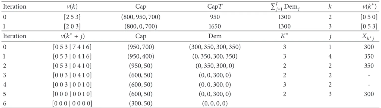
Table 2: Trace table of decoding procedure Iteration.
Iteration V(𝑘) Cap Cap𝑇 ∑𝐽𝑗=1Dem𝑗 𝑘 V(𝑘∗)
0 [2 5 3] (800, 950, 700) 950 1300 2 [0 5 0]
1 [2 0 3] (800, 0, 700) 1650 1300 3 [0 5 3]
Iteration V(𝑘∗+ 𝑗) Cap Dem 𝐾∗ 𝑗 𝑋𝑘∗𝑗
0 [0 5 3|7 4 1 6] (950, 700) (300, 350, 300, 350) 3 1 300 1 [0 5 3|0 4 1 6] (950, 400) (0, 350, 300, 350) 3 4 350 2 [0 5 3|0 4 1 0] (950, 50) (0, 350, 300, 0) 2 2 350 3 [0 0 3|0 4 1 0] (600, 50) (0, 0, 300, 0) 2 2 -4 [0 0 3|0 0 1 0] (600, 50) (0, 0, 300, 0) 3 2 -5 [0 0 0|0 0 1 0] (600, 50) (0, 0, 300, 0) 2 3 300 6 [0 0 0|0 0 0 0] (300, 50) (0, 0, 0, 0)
source (3) and the demand of depot (4) are updated. This sequence of operations is repeated until all demand of depots is satisfied and all priorities are reduce to zero. Table 2 presents the trace table for the example two-level supply chain network given in Figure 3 to show how its modified priority-based encoding is obtained. In this table, column V(𝑘) denotes the priority of the source nodes whileV(𝑘∗) denotes the priority values of the sources which will serve and set the others to zero. The capacity of the sources, the total capacity of the selected nodes, and demand vectors are given in columns Cap, Cap𝑇, and Dem, respectively. ColumnV(𝑘∗ + 𝑗) gives the representation and column𝐾∗nominate the selected source whereas column𝑋𝑘∗𝑗shows the flow amount
from the source𝑘∗to the demand node𝑗.
The decoding algorithm for representation of a two-level supply chain network is indicated in Algorithm 1. The representation should be divided to four segments to apply the above-presented decoding algorithm to the discussed CLSC network design.
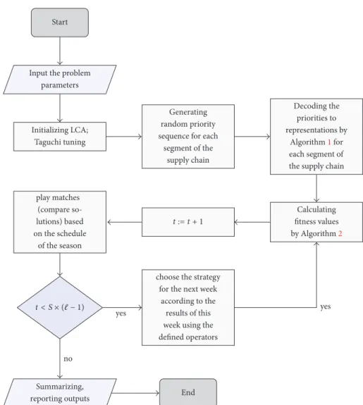
Decoding of the second segment of the representation is impossible until the first segment is decoded because customers demands consist of new products and recovered products, and the amount of recovered products is achieved only by decoding the first segment. Then, decoding of the third and fourth segments starts after determining the number and location of collection centers and the amount of the returned products. Decoding algorithm of representation for multilevel CLSC network is provided in Algorithm 2. 5.2. Discrete League Championship Algorithm. The LCA, first presented by Kashan [36], is a population-based algorithm for global search in a continuous space, which is inspired by the championship process of sports leagues in the real world. One of the common characteristics shared by all population-based algorithms such as LCA is their attempt to move a population of possible solutions to a number of promising areas in search of a desirable solution. Similar to many population-based algorithms, a set ofℓsolutions from the search space is randomly selected, which constitutes the initial population in the algorithm. Each solution obtained
from the population is related to one of ℓ teams (ℓ is an even number) that shows the current formation of the team. Hence, team𝑖represents𝑖th member of the population. Each solution obtained from the population has its own fitness value. In this algorithm, different solutions can be provided for a problem, which are compared on the basis of their fitness values (their objective function values). Each of the solutions is improved and ultimately near-optimal solution is selected. A number of teams (examined random initial solutions) compete together in a pairwise form as a league within a few weeks (the number of evaluation steps in an iterative algorithm). Winner and loser teams are determined (draw is not allowed) based on their power of play (metaphor of the fitness or objective value of the solution) resulting from the team formation. Every week, each team forms a new team formation by its coach with an artificial process analyzing the last week’s matches and obtains the best recognized formation up to that time (iterations number of the algorithm), and this process will continue. A schematic overview of our algorithm is given in Figure 4.
Parameters𝑆(examined number of seasons) andℓ(the number of teams) and constant coefficients used to scale the contribution of the strength and weakness of components (denoted by 𝜓1 and 𝜓2), are adjustable parameters whose changes have a direct impact on the final answer of the algo-rithm. The solution space in the CLSC problem is discrete, which means that components of each individual solution within the population cannot get an arbitrary amount, and they are allowed only to get natural values. Hence, a discrete LCA is dealt with to solve the CLSC problem. In addition, the numbers in representations should not be repeated. In the conducted studies dealing with discrete league championship algorithm, the algorithm searches a continuous space and finally presents a discrete solution by an innovative method. However, in the procedure proposed in the present study, all stages of the algorithm are made in the discrete space with no changes in the presentation of solution.
Hence, according to the discrete structure of the problem and the definition of team formation, discrete version of the operators (including addition, multiplication, subtraction, and arranging) is defined to address the strategies used in LCA in an appropriate structure to solve the CLSC problem.
Require:Gets𝐾̃: Set of sources,̃𝐽: Set of depots, Dem𝑗: demand on depot𝑗, Cap𝑘: capacity of source𝑘 Ensure:gives𝑈̃𝑘𝑗: Quantity of shipment between source𝑘and depot𝑗
(1) Cap𝑇 := 0,𝐾= 𝐾,𝐾= 0 (2)whileCap𝑇 < ∑𝐽𝑗=1Dem𝑗do
(3) select a node on𝑛 =arg max{V(𝑘), 𝑘 ∈ 𝐾1} (4) 𝐾= 𝐾\ {𝑛} (5) 𝐾= 𝐾∪ {𝑛} (6) Cap𝑇 = ∑𝑛∈𝐾Cap𝑛 (7) end while (8) V(𝑛) = 0, ∀𝑛 ∈ 𝐾 (9) Tr𝑛𝑗= ∞, ∀𝑗 ∈ ̃𝐽, 𝑛 ∈ 𝐾 (10)𝑋𝑘𝑗= 0, ∀𝑗 ∈ 𝐽, 𝑘 ∈ 𝐾 (11) whileV(𝑛) ̸= 0, ∀𝑛 ∈ 𝐽 ∪ ̃𝐾do
(12) Select a node based on𝑛 =argmax{V(𝑡), 𝑡 ∈ ̃𝐾 + ̃𝐽} (13) if 𝑙 ∈ 𝑘a source is selected𝑘∗= 𝑛then
(14) 𝑗∗=arg min{Tr𝑘𝑗}, 𝑗 ∈ ̃𝐽select a depot with minimum transportation cost (15) elseIf 𝑛 ∈ 𝐽a depot is selected𝑗∗= 𝑛
(16) 𝑘∗=arg min{Tr𝑘𝑗| 𝑘 ∈ 𝐾}select a source with minimum transportation cost (17) end if
(18) 𝑈̃𝑘∗𝑗∗=min(Cap𝑘∗,Dem𝑗∗)
(19) Update demand and capacities: (20) Cap𝑘∗=Cap𝑘∗− ̃𝑈𝑘∗𝑗∗
(21) Dem𝑗∗=Dem𝑗∗− ̃𝑈𝑘∗𝑗∗
(22) If Cap𝑘∗= 0thenV(𝑘∗) = 0
(23) If Dem𝑗∗= 0thenV(𝑗∗) = 0 (24) end while
Algorithm 1: The decoding algorithm of each section of representation for two-level supply chain network.
Requires:problem parameters
Ensure:Calculating the objective function in the multi-level CLSC
(1) 𝑍𝑖= 0, 𝑊𝑘= 0; 𝐻𝑙= 0, 𝑋𝑖𝑗= 0, 𝑌𝑗𝑘= 0, 𝑆𝑘𝑖= 0, 𝑇𝑘𝑙= 0, ∀𝑖 ∈ 𝐼, 𝑗 ∈ 𝐽, 𝑘 ∈ 𝐾, 𝑙 ∈ 𝐿 (2) Calculate𝑌𝑗𝑘fl̃𝑈𝑗𝑘, ∀𝑗 ∈ 𝐽, 𝑘 ∈ 𝐾by Algorithm 1 (3) If ∑𝑗𝑌𝑗𝑘> 0then𝑊𝑘= 1 (4) Calculate𝑇𝑘𝑙fl̃𝑈𝑘𝑙, ∀𝑘 ∈ 𝐾, 𝑙 ∈ 𝐿by Algorithm 1 (5) If ∑𝑘𝑇𝑘𝑙> 0then𝐻𝑙= 1 (6) Calculate𝑋𝑖𝑗fl𝑈̃𝑖𝑗, ∀𝑖 ∈ 𝐼, 𝑗 ∈ 𝐽by Algorithm 1 (7) If ∑𝑗𝑋𝑖𝑗> 0then𝑍𝑖= 1 (8) Calculate𝑆𝑘𝑖, ∀𝑘 ∈ 𝐾, 𝑖 ∈ 𝐼by Algorithm 1 (9) Calculate the total cost:
(10) obj= ∑𝐼𝑖=1𝐸𝑖𝑍𝑖+ ∑𝐾𝑘=1𝑓𝑘𝑊𝑘+ ∑𝐿𝑙=𝑎𝐺𝑙𝐻𝑙+ ∑𝐼𝑖=1∑𝐽𝑗=1TPS𝑖𝑗𝑋𝑖𝑗 (11) + ∑𝐽𝑗=1∑𝐾𝑘=1TSC𝑗𝑘𝑋𝑗𝑘+ ∑𝐾𝑘=1∑𝐼𝑖=1TCP𝑘𝑖𝑋𝑘𝑖+ ∑𝐾𝑘=1∑𝐿𝑙=1TCD𝑘𝑙𝑋𝑘𝑙
Algorithm 2: The decoding algorithm of representation for multilevel CLSC network.
The mentioned operators and their corresponding arguments are summarized below:
(1) Arrange (formation, strategy)→Plus Formation (2) Subtraction (formation, formation)→Minus Strategy (3) Addition (strategy, strategy)→Plus Strategy
(4) Multiplication (real number, strategy)→Times Strategy
The strategy vector and the above mentioned operators will be mathematically defined.
5.2.1. Strategy Vector and Organization Operator (Arrange). The strategy vector, denoted by𝑆, should be defined in such a way that by applying to a team formation vector at any time step, another team formation is achieved. Thus, the strategy vector𝑆for each team is defined as a sequence of “displacements” of team formation components as follows:
Start
Input the problem parameters
Initializing LCA; Taguchi tuning
Generating random priority sequence for each
segment of the supply chain Decoding the priorities to representations by Algorithm 1 for each segment of the supply chain
Calculating fitness values by Algorithm 2 play matches (compare so-lutions) based on the schedule of the season
choose the strategy for the next week
according to the results of this week using the defined operators
Summarizing,
reporting outputs End
yes yes
no
t < S × ( − 1)
t:= t + 1
Figure 4: The overview of the LCA algorithm implementation.
where‖𝑆‖specifies the length of sequence. Applying strategy
𝑆to a vector of team formation means that the components of𝑖1 and𝑗1in the vector of team formation are “displaced” together and then their components𝑖2and𝑗2and𝑖3and𝑗3are “displaced” together up to𝑖‖𝑆‖and𝑗‖𝑆‖. Hence, organization operator, i.e., the sum of team formation with a strategy, is defined as a set of displacements specified by the strategy vector in the vector of team formation. For example, if
𝐹 = (1, 2, 3, 4, 5)is the vector of team formation and𝑆 =
((1, 2), (2, 3)) is the vector of strategy, then the following situations are achieved, respectively, by applying𝑆to𝐹:
Displacement (1) with (2):(2, 1, 3, 4, 5) Displacement (2) with (3):(3, 1, 2, 4, 5) Hence, arrange(𝐹, 𝑆) = 𝐹 + 𝑆 = (3, 1, 2, 4, 5)
Symmetry of a strategy vector𝑆is displayed as−𝑆, which means that the sequence of displacements in𝑆is considered reversely.
5.2.2. Subtraction Operator. If𝑥1and𝑥2are two vectors of a team formation, the difference between𝑥1and𝑥2is defined
in a way that𝑥2 − 𝑥1 is equal to the vector of strategy, 𝑆. If it is applied to𝑥1, 𝑥2 is achieved. The algorithm which calculates the difference between𝑥1and𝑥2should be chosen with consideration of
𝑥2− 𝑥1= − (𝑥2− 𝑥1)
𝑥1= 𝑥2→ 𝑥2− 𝑥1= 0 (13)
Value of zero is displayed with 0 and is equal to a null sequence.
5.2.3. Addition Operator. If𝑆1and𝑆2are two strategy vectors, sum of them is displayed as𝑆1⊕ 𝑆2and equals to the strategy vector which is achieved by connecting the displacement sequence of𝑆2 to the end of sequence in𝑆1. As some dis-placements cancel each others effects, the obtained sequence from connecting 𝑆2 to 𝑆1 can be smaller; for example, if
𝑆1 = ((1, 2), (2, 5))and𝑆2 = (2, 5), then we have S1 ⊕ 𝑆2 =
((1, 2), (2, 5), (2, 5)).
However, since two consecutive displacements(2, 5) can-cel each others effects, they can be deleted; hence,𝑆1⊕ 𝑆2 =
(1, 2). Therefore, in general, we have‖𝑆1⊕ 𝑆2‖ ≤ ‖𝑆1‖ + ‖𝑆2‖. In addition, for each strategy𝑆, we will have𝑆 ⊕ −𝑆 = 0.
5.2.4. Multiplication Operator. If𝑐is a real number and𝑆is a strategy vector, their multiplication,𝑐𝑆, is defined as follows depending on the value of𝑐.
(1) Case of0 ≤ 𝑐 < 1: in this case, it is assumed that‖𝑐𝑆‖ is equal to the integral part of the number𝑐‖𝑆‖; vector𝑆is truncated so that its length is equal to‖𝑐𝑆‖:
𝑐𝑆 = ((𝑖𝑘, 𝑗𝑘) , 𝑘 = (1, 2, . . . , ‖𝑐𝑆‖)) . (14) In the special case of𝑐 = 0, we have𝑐𝑠 = 0.
(2) Case of𝑐 ≥ 1: in this case, we have𝑐 = 𝑘 + 𝑐, where
𝑘 = ⌊𝑐⌋is a natural number and𝑐= 𝑐−⌊𝑐⌋ ∈ [0, 1]. Therefore,
𝑐𝑆is defined as follows:
𝑐𝑆 = 𝑆 ⊕ 𝑆 ⋅ ⋅ ⋅ 𝑆⏟⏟⏟⏟⏟⏟⏟⏟⏟⏟⏟⏟⏟⏟⏟⏟⏟
𝑘times
⊕ 𝑐𝑆. (15)
(3) Case of 𝑐 < 0: in this case, the multiplication is converted to one of the above-presented modes by writing𝑐𝑆 as(−𝑐)(−𝑆).
We have four strategies whose notations are inspired from SWOT (Strength, Weakness, Opportunity, Threats) analysis in strategic planning literature.𝑆/𝑂corresponds to the aggressive strategy in which the team is strong and the opponent is week while 𝑊/𝑇, in contrast, corresponds to a defensive strategy in which the team is in a weak mode and the opponent is strong (threat). Two other intermediate strategies are denoted by𝑆/𝑇and𝑊/𝑂corresponding toboth strongandboth weakmodes, respectively. Let𝑋𝑡+1𝑖 denote the formation of team𝑖in week𝑡and𝐵𝑡𝑖 be the best formation for team 𝑖 in week 𝑡. The constant coefficients 𝜓1 and 𝜓2 are used to scale the strength and weakness of components, respectively.𝑟1and𝑟2are uniform random numbers from the interval[0, 1].
With the application of the defined operators, equations related to strategies in discrete LCA algorithm will be written as follows.
(i) If both teams𝑖and𝑙in week𝑡win their games against teams𝑗and𝑘, then formation of team𝑖in week𝑡 + 1 with strategy𝑆/𝑇will be as follows:
𝑋𝑖𝑡+1= 𝐵𝑡𝑖+ (𝜓1𝑟1(𝐵𝑡𝑖− 𝐵𝑘𝑡) ⊕ 𝜓1𝑟2(𝐵𝑡𝑖− 𝐵𝑡𝑗)) . (16)
(ii) If team𝑖wins team𝑗and team𝑙loses against team𝑘in week𝑡, team formation of𝑖in week𝑡 + 1with strategy
𝑆/𝑂will be as follows:
𝑋𝑡+1𝑖 = 𝐵𝑡𝑖+ (𝜓2𝑟1(𝐵𝑡𝑘− 𝐵𝑡𝑖) ⊕ 𝜓1𝑟2(𝐵𝑡𝑖− 𝐵𝑡𝑗)) . (17)
(iii) If both teams𝑖and𝑙lose their games against teams𝑗 and𝑘in week𝑡, team formation of𝑖in week𝑡+1with strategy𝑊/𝑇will be as follows:
𝑋𝑡+1𝑖 = 𝐵𝑡
𝑖+ (𝜓1𝑟1(𝐵𝑡𝑘− 𝐵𝑡𝑖) ⊕ 𝜓2𝑟2(𝐵𝑡𝑖− 𝐵𝑡𝑗)) . (18)
(iv) If both teams𝑖and𝑙lose their games against teams𝑗 and𝑘in week𝑡, team formation𝑖in week𝑡 + 1with strategy𝑊/𝑂will be as follows:
𝑋𝑡+1𝑖 = 𝐵𝑡𝑖+ (𝜓2𝑟1(𝐵𝑡𝑘− 𝐵𝑡𝑖) ⊕ 𝜓2𝑟2(𝐵𝑡𝑗− 𝐵𝑡𝑖)) . (19)
6. Numerical Results
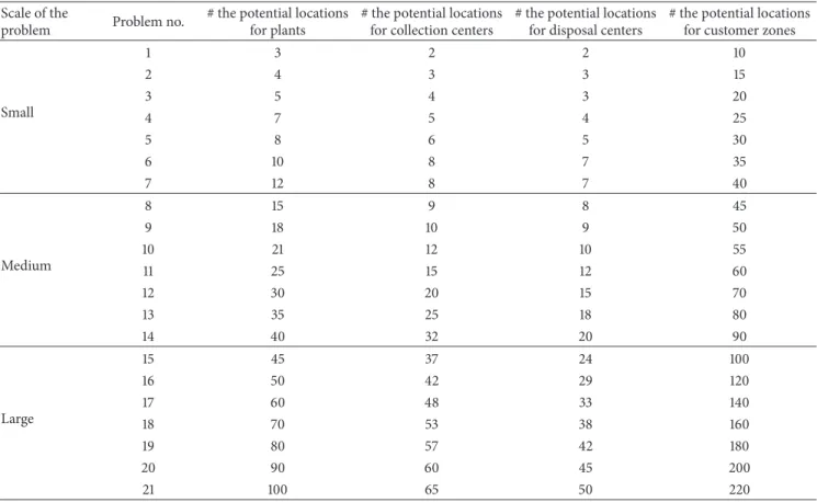
6.1. Problem Instances. In order to assess the performance of the proposed discrete LCA in terms of the objective-function value and CPU time, several numerical experiments with different problem sizes were implemented, and the obtained results are reported in this section. To this end, 21 sample problems with 3 different levels, which are small, medium, and large-scale problems, were generated by different combi-nations of the parameter values. The levels of the generated sample problems are shown in Table 3, and the ranges of the parameters are presented in Table 4. Furthermore, all parameters of the sample problems were randomly generated based on uniform distributions in prespecified intervals.
As the acquired results obtained from the proposed algorithm are sensitive to their initial parameters, any small changes can affect the accuracy of the best obtained solu-tion. Therefore, the Taguchi tuning method is used for the parameters to find the best solutions. In this method, first, the appropriate factors (initial parameters) are determined, the level of each factor is selected, and then the design of experiments for this control factor is specified. After specifying the experimental design, the proposed algorithm is used to find the best combination of factors. In our study, 4 levels are considered for each factor. In Table 5, the number of teams (ℓ), number of seasons (𝑆), and scaling constants of strength and weakness components (𝜓1and𝜓2) are given. 6.2. Objective Function Average. With respect to the pro-posed algorithm, the experimental design is employed according to the number of factors and number of levels. To this aim, each problem instance was solved five times to form the replications. Average results are reported as the final value. The best values of the proposed parameters for discrete LCA according to the mean normalized objective values are 150, 20, 6, and 2 for the number of teams, number of seasons, and constant coefficients to scale the contribution of the strength and weakness components, respectively. Moreover, Figure 5 presents the normalized average of means and the
𝑆/𝑁(Signal-to-noise) ratio graph for the experimental design of the algorithm. Based on the average of the means given in the graph, the algorithms result in a more efficient response if the parameter is placed in the lower level. Furthermore, in the 𝑆/𝑁 ratio graph, the algorithms result in a more efficient response if the parameter is placed in the higher level. According to Table 5 and Figure 5 the best performance of our algorithm is observed when the number of teams (ℓ) and the weakness scaling coefficient (𝜓2) are in level 2; the number of seasons (𝑆) is placed at level 1, and the strength scaling coefficient (𝜓4) is placed at level 4.
6.3. Solutions Structure and Quality. After tuning the param-eters of the proposed algorithm, PB3 results are compared
Table 3: Size and scale of sample problems. Scale of the
problem Problem no.
# the potential locations for plants
# the potential locations for collection centers
# the potential locations for disposal centers
# the potential locations for customer zones
Small 1 3 2 2 10 2 4 3 3 15 3 5 4 3 20 4 7 5 4 25 5 8 6 5 30 6 10 8 7 35 7 12 8 7 40 Medium 8 15 9 8 45 9 18 10 9 50 10 21 12 10 55 11 25 15 12 60 12 30 20 15 70 13 35 25 18 80 14 40 32 20 90 Large 15 45 37 24 100 16 50 42 29 120 17 60 48 33 140 18 70 53 38 160 19 80 57 42 180 20 90 60 45 200 21 100 65 50 220
Table 4: Pre-specified intervals to generate parameters intervals based on uniform distributions.
Parameter Range Parameter Range
𝐸𝑖 𝑈(1000000, 1200000) TSC𝑗𝑘 𝑈(20, 30) 𝐹𝑘 𝑈(1000000, 1200000) TCP𝑘𝑖 𝑈(20, 30) 𝐺𝑙 𝑈(1000000, 1200000) TCD𝑘𝑙 𝑈(20, 30) Dem𝑗 𝑈(100, 150) Cap𝑃𝑖 𝑈(800, 1200) 𝑟𝑗 𝑈(10, 50) Cap𝐶𝑘 𝑈(200, 400) 𝛽 𝑈(0.6, 0.8) Cap𝐷𝑙 𝑈(100, 300) TPS𝑖𝑗 𝑈(20, 30)
Table 5: Proposed parameter levels.
Parameter Level 1 Level 2 Level 3 Level 4
ℓ 100 150 200 25
𝑆 20 26 32 40
𝜓1 0 2 4 6
𝜓2 0 2 4 6
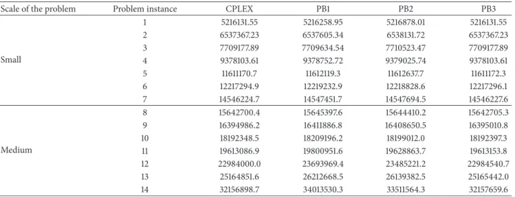
with those of the CPLEX outputs which were run on GAMS software (exact solution), PB2, and PB1 methods. For this purpose, five problem instances with random data given in Table 4 for each problem size given in Table 3 were generated, and they were solved by each method. The average of five problems were selected as the benchmark for each sample problem. In Table 6, the average results of each sample
problem instance is provided and compared with the solver’s (exact) solution.
According to the results shown in Table 6, it can be observed that the results of PB3 method are very close to the exact solution with a small deviation. The average deviations from the optimality for these algorithms are depicted in Figure 6, the solution obtained from PB3 algorithm for samples (1) to (4) are the same as the exact solution, as their deviations are zero. Furthermore, in comparison with the PB2 and PB3 methods, PB3 method resulted in smaller deviation values as the size of the problem increases. The optimality deviation in problem instance #14 is 760.9 (0.0024%) for PB3 algorithm while it is 1856631.6 (5.773%) and 1354665.6 (4.213%) units for PB1 and PB2 methods, respectively.
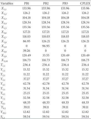
To demonstrate the difference between the output of the mentioned algorithms and the exact solution obtained from CPLEX, the solution of the problem instance (1) is reported in Table 7. According to this table, it is observed that all the three methods present the same number and locations for facilities. However, the difference is related to the quantity flow between facilities. The obtained quantity flow among facilities in PB3 methods and the exact solution is the same. 6.4. Convergence and Speed of Algorithms. To show the convergence rate of the algorithms and their quality, one of the problem instances, namely, instance #12, is used to demonstrate the performance of the proposed algorithms in Figure 7. The optimality gap is shown for each of the iterations
Table 6: The average of the objective values for each sample problem instance.
Scale of the problem Problem instance CPLEX PB1 PB2 PB3
Small 1 5216131.55 5216258.95 5216878.01 5216131.55 2 6537367.23 6537605.34 6538131.72 6537367.23 3 7709177.89 7709634.54 7710523.47 7709177.89 4 9378103.61 9378752.72 9379025.74 9378103.61 5 11611170.7 11612119.3 11612637.7 11611172.3 6 12217294.9 12219232.9 12218828.6 12217296.1 7 14546224.7 14547451.7 14547694.5 14546227.6 Medium 8 15642700.4 15645397.6 15644410.2 15642705.3 9 16394986.2 16411886.8 16408650.5 16395010.8 10 18192348.5 18209196.2 18199012.0 18192397.3 11 19613086.9 19800951.6 19628863.7 19613153.8 12 22984000.0 23693969.4 23485221.2 22984540.7 13 25164851.6 26212668.5 26139382.5 25165442.0 14 32156898.7 34013530.3 33511564.3 32157659.6
Main Effects Plot for Means
Data Means
Main Effects Plot for SN ratios
Data Means Me an o f Me an s M ea n o f S N ra tios 0.15 0.20 0.25 0.30 0.35 0.15 0.20 0.25 0.30 0.35 S S 10.0
Signal-to-noise: smaller is better 12.5 15.0 17.5 20.0 10.0 12.5 15.0 17.5 20.0 2 3 4 1 1 2 3 4 1 2 2 3 4 1 2 2 3 4 1 1 2 3 4 1 2 3 4 1 1 2 3 4 1 2 3 4
Figure 5: Means of means and the S/N ratio plot for discrete LCA.
and it is clearly observable that PB3 method is able to further search the solution space, which raise the chance of obtaining the optimal solution.
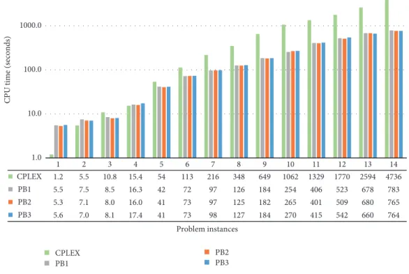
The computational time of the algorithms is another interesting factor to point out specially in NP-hard problems. The average computational time of our algorithms for each problem instance is given in Figure 8. According to this figure it is observed that the computational time of the exact solution increases exponentially as the size of the problem increases. The computational time of the exact solution has become more than that of PB1, PB2, and PB3 methods from the problem instance #3 onwards. This time increase shows that the exact solution is inefficient in solving large-scale problems and even it may not achieve the optimal solution. However, the computational times of PB1, PB2, and PB3 algorithms are close to each other and they are less than the solver’s except for some very small size problem instances. Generally, the study revealed that the proposed solution method has obtained results very close to those of the exact solution than the other methods. However, its computational time at large sizes is less than that of the exact solution.
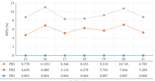
6.5. Algorithms Performance for Larger Scale Problems. To evaluate the performance of the proposed solution method for large-scale instances, 7 sample problems were solved using PB1, PB2, and PB3 algorithms each of them five times. As the solver could not find a feasible solution, the performance comparison on the solution quality is made using RPD measure which is defined below:
% RPD=Solmethod−BestSol
BestSol × 100, (20) where Solmethod is the solution obtained by each algorithm
and BestSol is the best solution obtained among all three solution methods. Table 8 presents the computational results in large-scale problems.
Figures 9-10 present a schematic comparison of the average CPU time and the average RPD value of three solution methods, respectively.
6.6. Statistical Analysis. We have used Duncan’s multiple range test as a statistical technique to compare the average results of each problem instance to conclude about the
Table 7: The location and quantity flow between facilities in problem instance #1. Variables PB1 PB2 PB3 CPLEX 𝑋1,1 133.96 133.96 133.96 133.96 𝑋3,2 126.2 126.2 126.2 126.2 𝑋3,3 104.18 104.18 104.18 104.18 𝑋3,4 128.34 128.34 128.34 128.34 𝑋1,5 135.56 135.56 135.56 135.56 𝑋3,6 127.21 127.21 127.21 127.21 𝑋3,7 118.03 118.03 118.03 118.03 𝑋1,8 86.95 126.21 126.21 126.21 𝑋1,9 0 96.95 0 0 𝑋3,8 39.26 0 0 0 𝑋3,9 120.49 33.55 120.49 120.49 𝑋3,10 116.73 116.73 116.73 116.73 𝑇1,1 236.4 236.4 236.4 236.4 𝑌1,1 15.32 15.32 15.32 15.32 𝑌2,1 11.22 11.22 11.22 11.22 𝑌3,1 37.27 37.27 37.27 37.27 𝑌4,1 42.78 42.78 42.78 42.78 𝑌5,1 31.34 31.34 31.34 31.34 𝑌6,1 25.15 25.15 25.15 25.15 𝑌7,1 32.58 32.58 32.58 32.58 𝑌8,1 48.33 48.33 48.33 48.33 𝑌9,1 39.11 39.11 39.11 39.11 𝑌10,1 12.82 12.82 12.82 12.82 𝑆1,1 59.54 59.54 59.54 59.54
Table 8: The average of the objective values for each problem instance (in large scale problems).
Problem instance # PB1 PB2 PB3 15 36913935 35518893 33938760 16 40865814 39330392 36800070 17 45761578 44397034 42238210 18 49926096 48933683 46045200 19 58336893 56463500 53420906 20 64568402 62410560 58308146 21 69765594 67512119 64137591
performance of the solution methods. The steps of Duncan’s multiple range test are as follows:
(1) Create a tree diagram, whose first node includes the average of𝐾treatments. Then, sort them in an increasing form and call it𝑝level.
(2) Create two branches from the first node. The first node includes the average of treatment 1 to𝐾 − 1, and the second node includes the average of treatment 2 to𝐾. Then, call it𝑝 − 1level.
(3) Proceed with step (2) pattern to the point that there are only two pairs of each node.
1 9 81 729 6561 59049 531441 4782969 1 2 3 4 5 6 7 8 9 10 11 12 13 14 Op timali ty de via tio n Problem Instances PB1 PB2 PB3
Figure 6: The average optimality deviation of the solutions obtained by each solution method within the small and medium size problem instances. 25 100 400 1600 6400 25600 102400 409600 1638400 6553600 0 25 50 75 100 125 150 Iteration PB3 PB2 PB1 Op timali ty de via tio n
Figure 7: The gap between the optimal objective value and the output of the three algorithms over the iterations for a problem instance.
(4) Calculate the range of𝑅for each branch of𝑝level in the tree chart using the following equation:
𝑅𝑝 =𝑆𝑒𝑟𝛼,𝑝,𝑑𝑓𝑒
√𝑛 , (21)
where𝑆𝑒is the standard error in the ANOVA,𝑛is the number of observations in each treatment, and the values of𝑟𝛼,𝑝,𝑑𝑓𝑒 are obtained from Duncan’s multiple range test table for the corresponding𝛼 value.𝑟𝛼,𝑝,𝑑𝑓𝑒 depends on the significance level 𝛼, the number of treatments 𝑝 at the node, and the degrees of freedom of the error,𝑑𝑓𝑒, for the ANOVA.
(1) Start from the first node and compare the𝑅value with the least significant level of𝑅𝑝Duncan.
(a) If 𝑅 > 𝑅𝑝, it can be concluded that the two averages are significantly different at the beginning and end of𝑝level node. Thus, apply
1 2 3 4 5 6 7 8 9 10 11 12 13 14 CPLEX 1.2 5.5 10.8 15.4 54 113 216 348 649 1062 1329 1770 2594 4736 PB1 5.5 7.5 8.5 16.3 42 72 97 126 184 254 406 523 678 783 PB2 5.3 7.1 8.0 16.0 41 73 97 125 182 265 401 509 680 765 PB3 5.6 7.0 8.1 17.4 41 73 98 127 184 270 415 542 660 764 1.0 10.0 100.0 1000.0 10000.0 CP U tim e (seconds) Problem instances CPLEX PB1 PB2 PB3
Figure 8: The average computational time of methods for each sample problem.
1000 1100 1200 1300 1400 1500 1600 1700 1800 1900 15 16 17 18 19 20 21 CPU T ime (s eco n ds) Sample Problem PB1 PB2 PB3
Figure 9: The average CPU-Time of each solution method in each large-scale problems.
this test to the next nodes, which is shown by Yes.
(b) If𝑅 < 𝑅𝑝, it can be concluded that there is no significant difference between the averages of𝑝 level node. Thus, do not apply this test to the next nodes, which is shown by No.
In our test, the aforementioned solution methods were compared via 21 sample problems and the results are reported in Table 9. For example, in the problem instance #12, it can
Table 9: The results of the Duncan test among each solution method. Problem instance # PB1 v.s. PB2 PB1 v.s. PB3 PB2 v.s. PB3 1 NO NO NO 2 NO NO NO 3 NO NO NO 4 NO NO NO 5 NO YES YES 6 NO YES YES 7 NO YES NO 8 NO NO YES 9 NO NO NO 10 NO YES YES 11 NO YES YES 12 NO YES YES 13 NO YES YES 14 NO YES YES 15 NO YES YES 16 NO YES YES
17 YES YES YES
18 YES YES YES
19 YES YES YES
20 YES YES YES
21 YES YES YES
be seen that there is a significant difference between the averages obtained from application of PB3 and PB2 methods
15 16 17 18 19 20 21 PB1 8.770 11.053 8.346 8.433 9.210 10.745 8.783 PB2 4.659 6.880 5.116 6.278 5.703 7.044 5.269 PB3 0.003 0.004 0.004 0.004 0.007 0.007 0.008 0 2 4 6 8 10 12 RPD (%) Problem Instance PB1 PB2 PB3
Figure 10: The average RPD of each solution method in each large-scale problems.
while there is no significant difference between the averages obtained from application of PB2 and PB1 methods.
7. Conclusion and Suggestions for
Future Studies
In this paper, a CLSC network including levels of the plants to customer zones, customer zones to collection centers, collection centers to plants, and collection centers to dis-posal centers was considered. We proposed a mathematical programming model and then developed a new population-based algorithm called the LCA to solve the model.
The proposed solution algorithm was designed by mod-ifying an existing LCA in the literature which is for con-tinuous space. We defined new operators and used them to convert the continuous space into the discrete one and hence we named our algorithm discrete LCA. We also proposed a new priority-based encoding for solving the problems. To demonstrate the effectiveness of the proposed method, an experimental study was conducted to study the small, medium, and large-scale problem instances. The numerical study showed that the outputs of our solution method is very close to the exact optimal solution which are obtained from the solver while it is significantly faster for large size problem instances. Furthermore, from the aspect of objective value, our proposed encoding method outperforms the two other existing methods in the literature which we referred to as PB1 and PB2 within the text whereas there are no significant differences between their computational time.
This work can be extended either with augmenting the model assumption or from the solution approach. For instance, considering a multiobjective model which addresses the sustainability concerns in supply chain network design, either from the customer viewpoint or from the suppliers,
would be an interesting problem to investigate in this frame-work. In addition, considering uncertainty in the demands and the returned-products can result in a more realistic and challenging problem to deal with.
Data Availability
The data used to support the findings of this study are available from the corresponding author upon request.
Conflicts of Interest
The authors declare that they have no conflicts of interest.
Acknowledgments
The research described in this paper was funded by Irans National Elites Foundation, I.R. IRAN, which is gratefully acknowledged here.
References
[1] K. Govindan, H. Soleimani, and D. Kannan, “Reverse logistics and closed-loop supply chain: a comprehensive review to explore the future,”European Journal of Operational Research, vol. 240, no. 3, pp. 603–626, 2015.
[2] M. Zohal and H. Soleimani, “A hybrid heuristic algorithm for the multistage supply chain network problem,” The Interna-tional Journal of Advanced Manufacturing Technology, vol. 26, no. 5, pp. 675–685, 2005.
[3] F. Du and G. W. Evans, “A bi-objective reverse logistics net-work analysis for post-sale service,”Computers & Operations Research, vol. 35, no. 8, pp. 2617–2634, 2008.
[4] V. Jayaraman, R. A. Patterson, and E. Rolland, “The design of reverse distribution networks: models and solution procedures,”
European Journal of Operational Research, vol. 150, no. 1, pp. 128–149, 2003.
[5] H. R. Krikke, A. Van Harten, and P. C. Schuur, “Business case Oc´e: reverse logistic network re-design for copiers,”OR Spectrum, vol. 21, no. 3, pp. 381–409, 1999.
[6] O. Listes¸ and R. Dekker, “A stochastic approach to a case study for product recovery network design,”European Journal of Operational Research, vol. 160, no. 1, pp. 268–287, 2005. [7] N. Aras, D. Aksen, and A. G. Tanu˘gur, “Locating collection
centers for incentive-dependent returns under a pick-up policy with capacitated vehicles,” European Journal of Operational Research, vol. 191, no. 3, pp. 1223–1240, 2008.
[8] H. ¨Uster, G. Easwaran, E. Akc¸ali, and S. C¸ etinkaya, “Benders decomposition with alternative multiple cuts for a multi-product closed-loop supply chain network design model,”Naval Research Logistics (NRL), vol. 54, no. 8, pp. 890–907, 2007. [9] Z. Lu and N. Bostel, “A facility location model for logistics
systems including reverse flows: the case of remanufacturing activities,”Computers & Operations Research, vol. 34, no. 2, pp. 299–323, 2007.
[10] R. Wojanowski, V. Verter, and T. Boyaci, “Retail-collection net-work design under deposit-refund,”Computers & Operations Research, vol. 34, no. 2, pp. 324–345, 2007.
[11] M. S. Pishvaee, K. Kianfar, and B. Karimi, “Reverse logistics network design using simulated annealing,”The International Journal of Advanced Manufacturing Technology, vol. 47, no. 1-4, pp. 269–281, 2010.
[12] X. Bing, J. M. Bloemhof-Ruwaard, and J. G. A. J. Van Der Vorst, “Sustainable reverse logistics network design for household plastic waste,”Flexible Services and Manufacturing Journal, vol. 26, no. 1-2, pp. 119–142, 2014.
[13] M. I. Gomes, A. P. Barbosa-Povoa, and A. Q. Novais, “Modelling a recovery network for WEEE: A case study in Portugal,”Waste Management, vol. 31, no. 7, pp. 1645–1660, 2011.
[14] S. A. Alumur, S. Nickel, F. Saldanha-da-Gama, and V. Verter, “Multi-period reverse logistics network design,”European Jour-nal of OperatioJour-nal Research, vol. 220, no. 1, pp. 67–78, 2012. [15] G. Kannan, P. Sasikumar, and K. Devika, “A genetic algorithm
approach for solving a closed loop supply chain model: a case of battery recycling,”Applied Mathematical Modelling: Simulation and Computation for Engineering and Environmental Systems, vol. 34, no. 3, pp. 655–670, 2010.
[16] B. C. Giri and S. Sharma, “Optimizing a closed-loop supply chain with manufacturing defects and quality dependent return rate,”Journal of Manufacturing Systems, vol. 35, pp. 92–111, 2015. [17] R. K. Pati, P. Vrat, and P. Kumar, “A goal programming model for paper recycling system,”Omega, vol. 36, no. 3, pp. 405–417, 2008.
[18] M. Godichaud and L. Amodeo, “Efficient multi-objective opti-mization of supply chain with returned products,”Journal of Manufacturing Systems, vol. 37, pp. 683–691, 2015.
[19] M. C. Fonseca, ´A. Garca-S´anchez, M. Ortega-Mier, and F. Saldanha-da Gama, “A stochastic bi-objective location model for strategic reverse logistics,”TOP, vol. 18, no. 1, pp. 158–184, 2010.
[20] E. ¨Ozceylan, T. Paksoy, and T. Bektas¸, “Modeling and optimiz-ing the integrated problem of closed-loop supply chain network design and disassembly line balancing,”Transportation Research Part E: Logistics and Transportation Review, vol. 61, pp. 142–164, 2014.
[21] H. Soleimani, M. Seyyed-Esfahani, and G. Kannan, “Incor-porating risk measures in closed-loop supply chain network design,”International Journal of Production Research, vol. 52, no. 6, pp. 1843–1867, 2014.
[22] P. Assarzadegan and M. Rasti-Barzoki, “Minimizing sum of the due date assignment costs, maximum tardiness and distribution costs in a supply chain scheduling problem,” Applied Soft Computing, vol. 47, pp. 343–356, 2016.
[23] F. T. S. Chan, A. Jha, and M. K. Tiwari, “Bi-objective optimiza-tion of three echelon supply chain involving truck selecoptimiza-tion and loading using NSGA-II with heuristics algorithm,”Applied Soft Computing, vol. 38, pp. 978–987, 2016.
[24] S. H. Amin and G. Zhang, “A multi-objective facility location model for closed-loop supply chain network under uncertain demand and return,” Applied Mathematical Modelling: Sim-ulation and Computation for Engineering and Environmental Systems, vol. 37, no. 6, pp. 4165–4176, 2013.
[25] M. Gen, F. Altiparmak, and L. Lin, “A genetic algorithm for two-stage transportation problem using priority-based encoding,” OR Spectrum, vol. 28, no. 3, pp. 337–354, 2006.
[26] A. Costa, G. Celano, S. Fichera, and E. Trovato, “A new efficient encoding/decoding procedure for the design of a supply chain network with genetic algorithms,” Computers & Industrial Engineering, vol. 59, no. 4, pp. 986–999, 2010.
[27] R. Jamshidi, S. M. T. F. Ghomi, and B. Karimi, “Multi-objective green supply chain optimization with a new hybrid memetic algorithm using the Taguchi method,”Scientia Iranica, vol. 19, no. 6, pp. 1876–1886, 2012.
[28] P. Subramanian, N. Ramkumar, T. T. Narendran, and K. Ganesh, “PRISM: PRIority based SiMulated annealing for a closed loop supply chain network design problem,”Applied Soft Computing, vol. 13, no. 2, pp. 1121–1135, 2013.
[29] M. Zohal and H. Soleimani, “Developing an ant colony approach for green closed-loop supply chain network design: a case study in gold industry,”Journal of Cleaner Production, vol. 133, pp. 314–337, 2016.
[30] M. Zandieh and A. Chensebli, “Reverse logistics network design: a water flow-like algorithm approach,”OPSEARCH, vol. 53, no. 4, pp. 667–692, 2016.
[31] R. Singh, A. Chakraborty, M. Kosambia, P. Shah, and A. Karhade, “Reverse logistics using genetic algorithm,” Interna-tional Journal of Innovative Research and Development, vol. 5, no. 2, 2016.
[32] S. H. R. Pasandideh and K. Asadi, “A priority-based modified encoding–decoding procedure for the design of a bi-objective sc network using meta-heuristic algorithms,”International Journal of Management Science and Engineering Management, vol. 11, no. 1, pp. 8–21, 2016.
[33] P. S. Davis and T. L. Ray, “A branch-bound algorithm for the capacitated facilities location problem,”Naval Research Logistics Quarterly, vol. 16, no. 3, pp. 331–344, 1969.
[34] M. Gen and R. Cheng, Genetic Algorithms and Engineering Optimization, vol. 7, John Wiley & Sons, 2000.
[35] Z. Michalewicz, G. A. Vignaux, and M. Hobbs, “Nonstandard genetic algorithm for the nonlinear transportation problem,” ORSA Journal on Computing, vol. 3, no. 4, pp. 307–316, 1991. [36] A. H. Kashan, “League Championship Algorithm: a new
algo-rithm for numerical function optimization,” inProceedings of the International Conference on Soft Computing and Pattern Recognition (SoCPaR ’09), pp. 43–48, IEEE, Malacca, Malaysia, December 2009.
Hindawi www.hindawi.com Volume 2018
Mathematics
Journal of Hindawi www.hindawi.com Volume 2018 Mathematical Problems in Engineering Applied Mathematics Hindawi www.hindawi.com Volume 2018Probability and Statistics Hindawi
www.hindawi.com Volume 2018
Hindawi
www.hindawi.com Volume 2018
Mathematical PhysicsAdvances in
Complex Analysis
Journal ofHindawi www.hindawi.com Volume 2018
Optimization
Journal of Hindawi www.hindawi.com Volume 2018 Hindawi www.hindawi.com Volume 2018 Engineering Mathematics International Journal of Hindawi www.hindawi.com Volume 2018 Operations Research Journal of Hindawi www.hindawi.com Volume 2018Function Spaces
Abstract and Applied AnalysisHindawi www.hindawi.com Volume 2018 International Journal of Mathematics and Mathematical Sciences Hindawi www.hindawi.com Volume 2018
Hindawi Publishing Corporation
http://www.hindawi.com Volume 2013 Hindawi www.hindawi.com
World Journal
Volume 2018 Hindawiwww.hindawi.com Volume 2018Volume 2018
Numerical Analysis
Numerical Analysis
Numerical Analysis
Numerical Analysis
Numerical Analysis
Numerical Analysis
Numerical Analysis
Numerical Analysis
Numerical Analysis
Numerical Analysis
Numerical Analysis
Numerical Analysis
Advances inAdvances in Discrete Dynamics in Nature and SocietyHindawi www.hindawi.com Volume 2018 Hindawi www.hindawi.com Differential Equations International Journal of Volume 2018 Hindawi www.hindawi.com Volume 2018