Intelligent Virtual Machine Placement for Cost
Efficiency in Geo-Distributed Cloud Systems
Kuan-yin Chen∗, Yang Xu∗, Kang Xi∗†, H. Jonathan Chao∗†
∗Polytechnic Institute of New York University, Brooklyn, New York 11201, USA †New York University Abu Dhabi, Abu Dhabi, UAE
Email: [email protected],{yangxu, kxi, chao}@poly.edu
Abstract— An important challenge of running large-scale cloud services in a geo-distributed cloud system is to minimize the over-all operating cost. The operating cost of such a system includes two major components: electricity cost and wide-area-network (WAN) communication cost. While the WAN communication cost is minimized when all virtual machines (VMs) are placed in one datacenter, the high workload at one location requires extra power for cooling facility and results in worse power usage effectiveness (PUE). In this paper, we develop a model to capture the intrinsic trade-off between electricity and WAN communication costs, and formulate the optimal VM placement problem, which is NP-hard due to its binary and quadratic nature. While exhaustive search is not feasible for large-scale sce-narios, heuristics which only minimize one of the two cost terms yield less optimized results. We propose a cost-aware two-phase metaheuristic algorithm, Cut-and-Search, that approximates the best trade-off point between the two cost terms. We evaluate Cut-and-Search by simulating it over multiple cloud service patterns. The results show that the operating cost has great potential of improvement via optimal VM placement. Cut-and-Search achieves a highly optimized trade-off point within reasonable computation time, and outperforms random placement by 50%, and the partial-optimizing heuristics by 10-20%.
Keywords-Geo-Distributed, Cloud System, Virtual Machine Placement, Resource Allocation, Electricity, Cost Optimization
I. INTRODUCTION
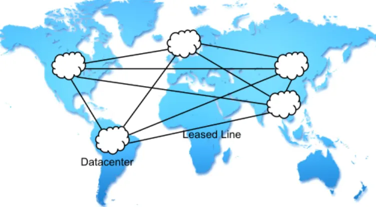
It is common practice for large cloud service providers (CSPs) to run their own geo-distributed cloud systems. Each cloud system consists of tens of geographically distributed datacenters interconnected with high-capacity WAN leased lines. For example, Google alone has deployed more than 30 datacenters worldwide [1], and Amazon Web Service (AWS) uses at least 20 [2]. An example of geo-distributed cloud system is shown in Figure 1. Some important reasons why CSPs adopt smaller, geo-distributed datacenters are: (1) Mega-datacenters are difficult to build, thus delay the time-to-market. (2) The requirements for space and cooling cause building costs to elevate as datacenters grow large [3]. (3) Physical limitations at a geographic region, such as land size and local energy availability.
Improving the cost of operating services is an important challenge for geo-distributed CSPs. It is because a CSP may provide a wide category of cloud services, such as content distribution, web storage, online collaboration and social net-working. These services are usually free or provided at a fixed
Fig. 1. An example of geo-distributed cloud system
monthly subscription charge, and cost optimization is subject to CSP’s discretion.
In this paper, we focus on two major contributors of cost during cloud service operation: (1)Electricity cost, the cost of powering VMs when they are instantiated in the datacenters. (2) WAN communication cost, incurred by communication between VMs across different datacenters. We choose the above two terms because they are recurring costs, which are repeatedly charged on CSPs as long as services continue, and can be adjusted by VM placement. Upfront captital costs, such as buildings and servers, are one-time costs. They are pretty much fixed before VM placement stage, and cannot be adjusted dynamically, and therefore are left out of the scope of our study. The VM placement problem is further motivated by the following observations:
1. Larger datacenters are power inefficient:[4] shows that the cooling facility can consume up to 33% of a datacen-ter’s power usage, compared to 30% by the servers. This significantly affects the power efficiency of a datacenter. The datacenter industry usually measures the power efficiency of a datacenter with the metric called power usage effectiveness
(PUE) [5], defined as follows:
PUE= Total datacenter power
Power consumed by IT equipments (1) Ideally all power consumed by a datacenter should go to the servers (PUE= 1.0). However, [5] reports that the PUE is close to 2.0 for conventional datacenters, while the best achievable case today is 1.13. The main reason for inflated
PUE values is cooling. Concentrating service workload at one datacenter can result in elevated demand for cooling, and thus worse datacenter PUE, and finally a penalizing electricity bill. To this end, [3] proposes to improve a datacenter’s power efficiency by distributing workload allocation to more locations. [6] pushes this concept to extreme by advocating the idea of nano datacenters, which are all-natural-cooling. Workload is distributed to a myriad of nano-datacenters and enjoy excellent power efficiency.
2. High WAN communication cost across datacenters: Usually a CSP connects its own geo-distributed datacen-ters with dedicated WAN links. Long-haul, inter-datacenter communication is significantly more expensive than intra-datacenter one [7][8]. For example, AWS [9] charges inter-datacenter transfer for $0.120-0.200/GB across geographic regions, $0.01/GB in the same region, and no charge for intra-datacenter communication. Due to such a large gap, a CSP may want to keep as much inter-VM communication inside datacenters as possible. This implies a more concentrated VM placement scheme.
There is intrinsic conflict between the two components in the operating cost. While a distributed VM placement results in favorable electricity cost, WAN communication cost is minimized when all VMs are put together. Minimizing one component may harm the optimality of the other. However, real service traffic patterns have shed some light on the op-timization problem. The inter-VM traffic profile of Microsoft Bing in [10] shows the following characteristics: (1) The inter-VM traffic matrix is very sparse. Very few of the inter-VM pairs actually communicates. (2) The VMs usually form multiple clusters. A majority of inter-VM traffic is with these clusters, while little traffic travels across clusters. These observations implicate that we only need to keep VMs in the same cluster in one datacenter to minimize WAN communication cost, instead of allocating everything to one location.
There are still some other factors to be considered. For example, the electricity price diversity at different locations. Take United States for example. The electricity prices at New York City (a.k.a. New Zone J Hub) is $62.71/MWh on-peak and $39.19/MWh off-peak, which are about double of the prices at Mid-Columbia Hub at Washington State, which are $29.10/MWh on-peak and $19.98/MWh off-peak.
We develop a model for VM placement in a geo-distributed cloud system, and introduce the Cost-Aware VM Placement Problem (CAVP). The objective of minimizing the operating cost. We will show that CAVP is NP-hard. Therefore, it is not practical to exhaustively search for optimum in large problem instances. We propose Cut-and-Search, a metaheuristic two-phase algorithm for solving CAVP. This scheme not only outperforms random placement by over 50% in the best case, but also have significant improvement over other partial-optimizing heuristics.
The contributions of this paper are as follows: (1) We develop a model for a geo-distributed cloud system capturing the intrinsic conflict between electricity and WAN communi-cation cost, then formulate it into the CAVP problem. (2) We
propose a cost-aware metaheuristic algorithm for CAVP, and demonstrate its performance.
The paper is organized as follows: Section II discusses related works of geo-distributed cloud computing and VM placement. Section III describes the system model we use and formulates the CAVP problem, with some notes on its complexity. In Section IV our algorithm, Cut-and-Search, is detailed. In Section V we evaluates Cut-and-Search against other heuristics. Concluding remarks are in Section VI.
II. RELATEDWORKS
Optimal resource placement in cloud services has been a topic gaining much attention today. [8] provides a back-of-the-envelope cost breakdown of data center operation, and indicates the possibility of cost reduction via optimal VM placement and datacenter sizing.
Several works have addressed intra-datacenter VM place-ment issue. [11] minimizes the bandwidth usage inside a single datacenter with traffic-aware VM placement. [12] proposes an abstraction for VM placement in order to provide guaranteed bandwidth to tenants and save datacenter network resource. [10] develops an optimization framework seeking the best trade-off between bandwidth reduction and fault tolerance. These works focus on intra-datacenter environments, while our work focuses on multi-datacenter system considering diversed power pricing and efficiency at different geographic locations. The workload placement problem is also extensively studied in the context of geo-distributed cloud systems. [13] optimally places VMs in distributed clouds with the main objective of minimizing the maximum latency (a.k.a. diameter) in VM clusters. [14] addresses the data placement issue for geo-distributed cloud services, and the main goal is to minimize the observed client request latency. These works focus on objectives related to inter-VM traffic, but do not pay attention to costs related to VM instance itself, such as electricity consumption.
There are several related works addressing optimal work-load placement in distributed datacenters with heterogeneous pricing scheme and resource constraints. [15] aims to find optimal resource placement and workload assignment in a content distribution network (CDN) to minimize the cost of content transfer to end users. [16] uses statistical multiplex-ing to mitigate bandwidth cost between datacenters and end users, and takes datacenters’ electricity price diversity into consideration. [17] cuts electricity bill by intuitively directing workload to the datacenters with lower spot prices. These works generally ignores inter-VM traffic and thus can only cover a part of overall operating cost in a geo-distributed cloud system.
To the best of our knowledge, our work is the first to consider both electricity cost and WAN communication cost, and address the intrinsic conflict between the two components, compared with works mentioned above most of which consider only part of the overall operating cost of a cloud system.
III. THECOST-AWAREVM PLACEMENTPROBLEM
A. System Model
We consider the scenario of deploying a large-scale cloud service in a geo-distributed cloud system. Table I summarizes the definitions and symbols used in problem formulation. 1. The cloud service pattern: Let V denote the set of V
VMs used by the cloud service, and v, v0 = 1,2, ..., V be the indices of these VMs. The power consumption of each VMv is denoted byPv. The bandwidth demand between any pair of VMs (v, v0)is denoted byTvv0.
2. The geo-distributed cloud system:LetDdenote the set of
D geo-distributed datacenters in the cloud system, andd, d0= 1,2, ..., Dbe the indices of datacenters. For datacenterd, the total power consumption is denoted byPd, the electricity price is Ed, and the quota of power provided by local grid is Qd. We assume that each pair of datacenters is connected by a dedicated WAN link. The links are billed based on the actual usage over a billing period. We denote the unit cost of data transfer between datacentersdandd0 byC
dd0. We ignore the costs of intra-datacenter communication, since it is very low compared with WAN. That is, Cdd = 0,∀d∈ D.
3. Modeling power efficiency at datacenters: We use the notation xvd to signal the allocation of VM v to datacenter
d. xvd = 1 when v is allocated to d, and 0 otherwise. The set of all xvd is called a state, denoted by X. We define the
workload atd as wd = P v∈V
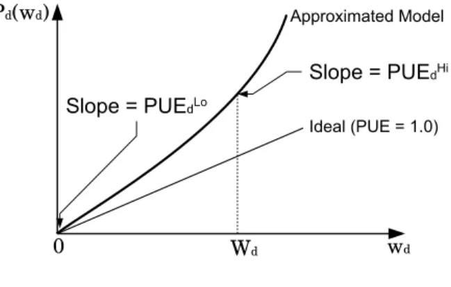
Pvxvd. [3][6] have demonstrated that when workload at a datacenter is low, it is possible to rely on natural cooling and eliminate cooling facility. We develop an approximate model as follows: For datacenter d, when wd ' 0, the cooling facility is off and the datacenter has a close-to-ideal PUE value, denoted by P U ELo
d . As wd increases, the demand for cooling rises and PUE increases. We assume that the measured value of PUE whenwd =Wd, the measured PUE value is P U EdHi. Then we approximate the relationship between Pd andwd with a quadratic polynomial function, defined as (2), and illustrated in Figure 2:
Pd(wd) =αwd2+βwd+γ (2)
α,β and are constants satisfying Pd0(Wd) = 2αWd+β=
P U EHi
d , and Pd0(0) =β = P U EdLo. The electricity cost at datacenterdis thusfd
E=Ed×Pd. We assume that datacenters can smartly turn off servers when there is zero load, and therefore γ= 0.
B. Problem Formulation
Refer to the symbol definitions in Table I, we propose and formulate the Cost-Aware VM Placement (CAVP)problem as follows:
Fig. 2. Relationship betweenPdandwd.
TABLE I
SYMBOLS USED INCAVPPROBLEM FORMULATION
Symbol Meaning
Input Parameters
V The set of VMs used by the cloud service D The set of datacenters in the cloud system v, v0= 1,2, ..., V The indices of VMs inV
d, d0= 1,2, ..., D The indices of datacenters inD
Pv Power consumption of VMv
Tvv0 Traffic demand between VMvandv0 Qd Quota of power provided to datacenterd wd Workload at datacenterd
Wd The point whenwd=Wd, PUE isP U EHi d Pd(wd) Total VM power consumption at datacenterd,
which is a function of placementwd Ed Electricity price at datacenterd
Cdd0 Unit transfer cost between datacentersdandd0 P U ELod , P U EHid PUE values at datacenterdatwd= 0, Wd Decision Variables
xvd Allocation of VMvto datacenterd 1 if allocated, 0 otherwise.
X Astate.X={xvd,∀v∈ V, d∈ D}
Cost Components
f(X) Total operating cost fE(X) Total electricity cost fC(X) Total communication cost fd
E Electricity cost at datacenterd
min X f(X) =fE(X) +fC(X) (3) fE(X) = X d∈D fEd(Pd) (4) fC(X) = 1 2 X v,v0∈V X d,d0∈D xvdxv0d0Tvv0Cdd0 (5) s. t. xvd={0,1} ∀v∈ V, d∈ D (6) X d∈D xvd= 1 ∀v∈ V (7) Pd≤Qd ∀d∈ D (8)
As described in (3), the CAVP problem’s objective is to minimize the geo-distributed cloud system’s operating cost. The details of electricity cost andWAN communication cost
is subject to the following constraints: All decision variables are binary integers, as indicated by (6). (7) ensures that every VM is assigned, and assigned to exactly one datacenter. (8) represents the constraints of power availability at each datacenter.
C. Problem Complexity and Scaling to Large Cloud Services
In CAVP’s formulation, all decision variables are binary integers. The objective function (3) contains quadratic terms of xvd. Therefore, the CAVP problem belongs to the category of Binary Quadratic Programming (BQP) problems. BQP problems are known to be NP-hard in general cases[18].
Large-scale cloud services usually use tens of thousands of VMs in total. Under such scale, solving the optimization prob-lem may still be computationally overwhelming. In practice, we can apply some coarsening preprocessing [10] to reduce the scale of problem instance. This can be done by greedily aggregating high communication VMs into small groups of a configurable size limit, and treat these groups as elemental unit of placement, i.e. VMs in CAVP problem formulation.
IV. ALGORITHM
CAVP is known to be NP-hard. Exhaustive search method is not feasible for problem scale larger than several tens of VMs [18]. Therefore our goal is to develop an approximation algorithm that significantly reduces operating cost within a reasonable computation time. We are motivated to take a
metaheuristic(iterative searching) approach due to the follow-ing facts: (1) fE(X) andfC(X) are intrinsically conflicting. Optimal trade-off is difficult to achieve with a straightforward heuristic. (2) The objective functionf(X)is aconvexfunction. No local minimum exists and anyneighbor statethat improves the cost is one step closer to the global minimum. A neighbor state is defined as any state that reallocates one VM to a different datacenter from the current state.
The most basic metaheuristic algorithm is greedy random walk (GRW), which randomly generates an initial state, and for each iteration, a neighbor state is generated and accepted as long as it decreases the cost. Our two-phase algorithm, CUT-and-Search, improves search efficiency by adopting two design principles: (1) Find a low starting point. In the first phase, we generate an initial placement having fC(X) optimized by a low-complexity graph partitioning algorithm. (2) Choose the best move. In the second phase, the algorithm iteratively searches among multiple neighbor states for the one having
steepest descent inf(X). The details of Cut-and-Search are as follows:
1. First phase: We consider the graph representation of the cloud service, G = (V,E). Each node v is assigned with a weight equal to Pv, and each edge (v, v0)has a weight equal toTvv0. We first min-cutGintoDpartitions,S1, S2, ..., SD, so that the weight sum of cross-partition edges is minimized. We then map partitions to datacenters bijectively. To avoid high-rising PUE, we start with a balanced cut, where each partition’s total power consumption is about the same value
L = P v∈V
Pv/D. This part is similar to the classic balanced
Algorithm 1 Phase 1-1: Grouping VMs
Input: G(V,E): Graph representation of cloud service as described in Section III-C.
L: Upper-bound of total power of each group. Output: S1, S2, ..., SD: VM groups.
1: V0← V
2: S1, S2, ..., SD←φ
3: power(Sy)←0 ∀y= 1,2, ..., D 4: while V0 not emptydo
5: fory= 1,2, ..., Ddo 6: v=argmax v∈V0 P v0∈V0,v06=v Tvv0 ! 7: AddT oGroup(v, Sy) 8: while∃v∈ V0, F it(v, Sy) = 1do 9: ˜v= argmax v∈V0,F it(v,S y)=1 P v0∈S Tvv0 10: AddT oGroup(˜v,Vy) 11: end while 12: end for 13: end while 14: function ADDTOGROUP(v, S) 15: S←S∪v,V0 ← V0−v 16: power(S) =power(S) +Pv 17: end function 18: function FIT(v, S)
19: ifpower(S) +Pv≤Lthen Return 1 20: elseReturn 0
21: end if 22: end function
Algorithm 2 Phase 1-2: Mapping groups to datacenters Input: S={S1, S2, ..., SD }: The set of unmapped
groups;D: Set of datacenters Output: X: Initial state
1: D0 ← D
2: while S not emptydo 3: S=argmax S∈S P v∈S,v0∈/S Tvv0 4: d=argmin d∈D0 P d06=d Cdd0 5: Allocate all VMs in S to d. 6: S ← S −S,D0 ← D0−d 7: end while
minimum k-cutproblem except that each node has a weightPv and that we limit the each partition by its total node weight, not number of VMs.
Algorithm 1 provides a greedy solution to the minimum-cut problem. At the start of creating a partitionS, the algorithm first identifies the unallocated VM that has maximum amount of traffic associated to it, and allocate it to the empty partition.
The algorithm then repeatedly finds and allocates to S the unallocated VM with most traffic to and from VMs are already in S, until no more VM can fit inS without breaking the L
limit. After D balanced partitions are constructed, Algorithm 2 optimizesfC(X)by greedily mapping the group with higher external traffic to the datacenter with smaller sum of unit transfer costs on links attached to it, and vice versa.
2. Second phase: The first phase has generated an initial placement with an minimized fC(X), but the overall cost
f(X)is yet taken care of. We further improve the result by iteratively searching for the neighbor state causing steepest descent inf(X). The large problem scale prevents the algo-rithm from exhaustively testing all possible neighbor states. In practice, during each iteration, we sampleNfeasible neighbor states, and accept the one with most negative ∆f(X). Since current state and the neighbor state differ only in one VM, ∆f(X) can be efficiently derived by calculating the partial costs associated with that VM. If no sampled moves reduce
f(X), we discard these samples and go to next iteration. The algorithm halts if it reaches I1 iterations, or f(X) remain
unchanged for I2 iterations. N, I1 and I2 are configurable
parameters.
V. PERFORMANCEEVALUATION
In this section, We evaluate Cut-and-Search by simulation over multiple cloud service patterns. We first describe the setup of simulation, then the results and related discussion.
A. Experiment Setup
1. Geo-Distributed Cloud Systems: We generate synthetic distributed cloud systems by randomly selecting D = 20 locations within mainland United States. For the electricity prices Ed, we incorporate the latest market data provided by Federal Energy Regulatory Commission (FERC) [19], and map each location to the nearest hub’s average spot price.
For WAN link bandwidth costs, we adopt a pricing model similar to Amazon EC2 Internet Data Transfer [9]. There is no charge for intra-datacenter (a.k.a. availability zone) communication; bandwidth cost is lower for links with short earth surface distance, and is much higher for long-haul links. 2. Cloud Service and Traffic Patterns: We design multiple cases of cloud services and their traffic patterns by following the observations made in [10]. We synthesize five data sets, of which the numbers of VMs and clusters are shown in Table II. The total number of VMs is fixed, but the clusters’ sizes can be different.
TABLE II
DATA SETS USED IN OUR SIMULATION
Data Set 1 2 3 4 5
# of VMs 1000
# of clusters 1 5 10 50 100
3. Benchmarks: We compare our solution with three other heuristics: Random Placement, and partial-optimizing algo-rithms like Greedy-Electricity-Cost (GEC) and Minimum-k-Cut. The GEC heuristic greedily optimizesfE(X)by
allocat-Fig. 3. Total costs resulting from different algorithms over multiple data sets. For each data set, the results are normalized to therandom placement
case.
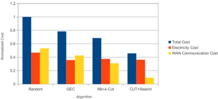
Fig. 4. Cost structure resulting from each algorithm on data set 3. All results are normalized tof(X)ofrandom placement.
ing VMs one by one to the datacenter with lowest ∆fE(X) available then, but pays no attention tofC(X). The Minimum-k-Cut heuristic minimizesfC(X)by applying Algorithm 1 and 2, but pays no attention to fE(X).
B. Evaluation Results
1. Total cost:In the first experiment, we synthesize a multitude of cloud service data sets. Five of these data sets are shown in Table II. The data sets are evaluated on a common 20-datacenter cloud system, and compare the total costs resulting from the four algorithms. The results are shown in Figure 3. As seen in Figure 3, Cut-and-Search outperforms random placement by 18% in f(X) improvement on data set 1, and more than 60% on data set 5. Our algorithm also outperforms
GECandMinimum k-cut by 10 to 20 %.
Cut-and-Search performs better in service scenarios with small-cluster traffic patterns. It is because with small clusters in traffic pattern, it is easier to put the whole cluster, and thus keep a large portion of inter-VM traffic inside datacenters, yielding very little WAN communication. On the contrary, with an all-to-all traffic pattern, like data set 1, Cut-and-Search can present less improvement, due to the fact that a considerable portion of traffic still has to travel the WAN links.
2. Looking into the cost structures: In the second experi-ment, we compare the cost structures resulting from the our heuristics and three other benchmarks on data set 3. The data
set has a 1000-VM traffic pattern divided into 50 clusters.
GEC achieves lowest fE(X) among all four algorithms as expected. However, Cut-and-Search compromises only slightly infE(X), but has much lowerfC(X). This indicates that only partially optimizing one of the two cost components is far from reaching the best trade-off between them.
3. Efficiency of iterative search: During the second phase algorithm, i.e. the iterative search, we sample N = 100 feasible moves in each iteration and sets termination condition to I1 = 30000iterations, or I2= 500 iterations without cost
change. On average, Cut-and-Search takes 76.96 seconds to complete in each run, and 13248 iterations to terminate.
VI. SUMMARY
In this paper, we consider the problem of placing VMs across multiple geo-distributed datacenters with the objective of optimizing the overall operating cost. In the CAVP prob-lem formulation, we capture the intrinsic trade-off between electricity cost and WAN communication cost, as well as the electricity price diversity at different geographic locations. Due to the NP-hardness, exhaustive search is not feasible. To this end, we develop Cut-and-Search, a two-phase metaheuristic algorithm that approaches optimal trade-off point and thus minimizes the operating cost.
We simulated Cut-and-Search against three other heuristics on multiple cloud service patterns. The results shows that the potential of performance improvement is significant, and partial-optimizing heuristics, such as Greedy-Electricity-Cost and Minimum k-cut, are not sufficient to reach best results.
VII. ACKNOWLEDGEMENTS
This research work is supported by NSF under grant CNS-1229218, and the NYU Abu Dhabi Institute under grant 73-71210-G1103.
REFERENCES
[1] R. Miller, “Google Data Center FAQ,” http://www.datacenterknowledge. com/archives/2008/03/27/google-data-center-faq/, Mar. 2008. [2] Amazon, “Amazon Global Infrastructure,” http://aws.amazon.com/
about-aws/globalinfrastructure/.
[3] K. Church, A. Greenberg, and J. Hamilton, “On Delivering Embar-rassingly Distributed Cloud Services,” in Seventh ACM/SIGCOMM Workshop on Hot Topics in Networks (HotNets 08), Oct. 2008. [4] BMC Software, “Data center cooling constraints,” http:
//discovery.bmc.com/confluence/display/Configipedia/Data+Center+ Cooling+Constraints, May 2009.
[5] Google, “Data center efficiency,” http://www.google.com/about/ datacenters/inside/efficiency/, Aug. 2012.
[6] V. Valancius, N. Laoutaris, L. Massoulie, C. Diot, and P. Rodriguez, “Greening the internet with nano data centers,” inCoNEXT ’09, Dec. 2009.
[7] A. Mahimkar, A. Chiu, R. Doverspike, M. D. Feuer, P. Magill, E. Mavro-giorgis, J. Pastor, S. L. Woodward, and J. Yates, “Bandwidth on demand for inter-data center communication,” inProc. 10th ACM Workshop on Hot Topics in Networks (HotNets ’11), 2011.
[8] A. Greenberg, J. Hamilton, D. A. Maltz, and P. Patel, “The cost of a cloud: research problems in data center networks,”SIGCOMM Comput. Commun. Rev., vol. 39, no. 1, pp. 68–73, Dec. 2008.
[9] Amazon, “Amazon ec2 pricing,” http://aws.amazon.com/ec2/pricing/, Aug. 2012.
[10] P. Bodik, I. Menache, M. Chowdhury, P. Mani, D. A. Maltz, and I. Stoica, “Surviving failures in bandwidth-constrained datacenters,” in
ACM SIGCOMM ’12, Aug. 2012.
[11] X. Meng, V. Pappas, and L. Zhang, “Improving the scalability of data center networks with traffic-aware virtual machine placement,” inIEEE INFOCOM 2010, 2010.
[12] H. Ballani, P. Costa, T. Karagiannis, and A. Rowstron, “Towards predictable datacenter networks,” inACM SIGCOMM ’11, 2011. [13] M. Alicherry and T. Lakshman, “Network aware resource allocation in
distributed clouds,” inIEEE INFOCOM 2012, 2012.
[14] S. Agarwal, J. Dunagan, N. Jain, S. Saroiu, A. Wolman, and H. Bhogan, “Volley: automated data placement for geo-distributed cloud services,” inUSENIX NSDI ’10, 2010.
[15] D. Applegate, A. Archer, V. Gopalakrishnan, S. Lee, and K. K. Ra-makrishnan, “Optimal content placement for a large-scale vod system,” inCoNEXT ’10, 2010.
[16] H. Xu and B. Li, “Cost efficient datacenter selection for cloud services,” in First IEEE International Conference on Communications in China, Aug. 2012.
[17] A. Qureshi, R. Weber, H. Balakrishnan, J. Guttag, and B. Maggs, “Cutting the electric bill for internet-scale systems,” inACM SIGCOMM ’09, 2009.
[18] K. Katayama and H. Narihisa, “Performance of simulated annealing-based heuristic for the unconstrained binary quadratic programming problem,”European Journal of Operational Research, vol. 134, no. 1, pp. 103–119, October 2001.
[19] Federal Energy Regulatory Commission, “Electric power markets: Overview,” http://www.ferc.gov/market-oversight/mkt-electric/ overview/2012/08-2012-elec-ovr-archive.pdf, Aug. 2012.