Creating Relational Data from Unstructured and
Ungrammatical Data Sources
Matthew Michelson [email protected]
Craig A. Knoblock [email protected]
University of Southern California Information Sciences Instistute 4676 Admiralty Way
Marina del Rey, CA 90292 USA
Abstract
In order for agents to act on behalf of users, they will have to retrieve and integrate vast amounts of textual data on the World Wide Web. However, much of the useful data on the Web is neither grammatical nor formally structured, making querying difficult. Examples of these types of data sources are online classifieds like Craigslist1 and auction item listings like eBay.2 We call this unstructured, ungrammatical data “posts.” The unstructured nature of posts makes query and integration difficult because the attributes are embedded within the text. Also, these attributes do not conform to standardized values, which prevents queries based on a common attribute value. The schema is unknown and the values may vary dramatically making accurate search difficult. Creating relational data for easy querying requires that we define a schema for the embedded attributes and extract values from the posts while standardizing these values. Traditional information extraction (IE) is inadequate to perform this task because it relies on clues from the data, such as structure or natural language, neither of which are found in posts. Furthermore, traditional information extraction does not incorporate data cleaning, which is necessary to accurately query and integrate the source. The two-step approach described in this paper creates relational data sets from unstructured and ungrammatical text by addressing both issues. To do this, we require a set of known entities called a “reference set.” The first step aligns each post to each member of each reference set. This allows our algorithm to define a schema over the post and include standard values for the attributes defined by this schema. The second step performs information extraction for the attributes, including attributes not easily represented by reference sets, such as a price. In this manner we create a relational structure over previously unstructured data, supporting deep and accurate queries over the data as well as standard values for integration. Our experimental results show that our technique matches the posts to the reference set accurately and efficiently and outperforms state-of-the-art extraction systems on the extraction task from posts.
1. Introduction
The future vision of the Web includes computer agents searching for information, making decisions and taking actions on behalf of human users. For instance, an agent could query a number of data sources to find the lowest price for a given car and then email the user the car listing, along with directions to the seller and available appointments to see the car.
1. www.craigslist.org 2. www.ebay.com
This requires the agent to contain two data gathering mechanisms: the ability to query sources and the ability to integrate relevant sources of information.
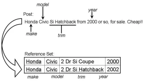
However, these data gathering mechanisms assume that the sources themselves are de-signed to support relational queries, such as having well defined schema and standard values for the attributes. Yet this is not always the case. There are many data sources on the World Wide Web that would be useful to query, but the textual data within them is un-structured and is not designed to support querying. We call the text of such data sources “posts.” Examples of “posts” include the text of eBay auction listings, Internet classifieds like Craigslist, bulletin boards such as Bidding For Travel3, or even the summary text below the hyperlinks returned after querying Google. As a running example, consider the three posts for used car classifieds shown in Table 1.
Table 1: Three posts for Honda Civics from Craigslist Craigslist Post
93 civic 5speed runs great obo (ri) $1800 93- 4dr Honda Civc LX Stick Shift $1800 94 DEL SOL Si Vtec (Glendale) $3000
The current method to query posts, whether by an agent or a person, is keyword search. However, keyword search is inaccurate and cannot support relational queries. For example, a difference in spelling between the keyword and that same attribute within a post would limit that post from being returned in the search. This would be the case if a user searched the example listings for “Civic” since the second post would not be returned. Another factor which limits keyword accuracy is the exclusion of redundant attributes. For example, some classified posts about cars only include the car model, and not the make, since the make is implied by the model. This is shown in the first and third post of Table 1. In these cases, if a user does a keyword search using the make “Honda,” these posts will not be returned. Moreover, keyword search is not a rich query framework. For instance, consider the query, What is the average price for all Hondas from 1999 or later? To do this with keyword search requires a user to search on “Honda” and retrieve all that are from 1999 or later. Then the user must traverse the returned set, keeping track of the prices and removing incorrectly returned posts.
However, if a schema with standardized attribute values is defined over the entities in the posts, then a user could run the example query using a simple SQL statement and do so accurately, addressing both problems created by keyword search. The standardized attribute values ensure invariance to issues such as spelling differences. Also, each post is associated with a full schema with values, so even though a post might not contain a car make, for instance, its schema does and has the correct value for it, so it will be returned in a query on car makes. Furthermore, these standardized values allow for integration of the source with outside sources. Integrating sources usually entails joining the two sources directly on attributes or translations of the attributes. Without standardized values and
a schema, it would not be possible to link these ungrammatical and unstructured data sources with outside sources. This paper addresses the problem of adding a schema with standardized attributes over the set of posts, creating a relational data set that can support deep and accurate queries.
One way to create a relational data set from the posts is to define a schema and then fill in values for the schema elements using techniques such as information extrac-tion. This is sometimes called semantic annotation. For example, taking the second post of Table 1 and semantically annotating it might yield “93- 4dr Honda Civc LX Stick Shift $1800 <make>Honda<\make> <model>Civc< \model> <trim>4dr LX<\trim> <year>1993< \year> <price>1800< \price>.” However, traditional information extrac-tion, relies on grammatical and structural characteristics of the text to identify the attributes to extract. Yet posts by definition are not structured or grammatical. Therefore, wrapper extraction technologies such as Stalker (Muslea, Minton, & Knoblock, 2001) or RoadRunner (Crescenzi, Mecca, & Merialdo, 2001) cannot exploit the structure of the posts. Nor are posts grammatical enough to exploit Natural Language Processing (NLP) based extraction techniques such as those used in Whisk (Soderland, 1999) or Rapier (Califf & Mooney, 1999).
Beyond the difficulties in extracting the attributes within a post using traditional ex-traction methods, we also require that the values for the attributes are standardized, which is a process known as data cleaning. Otherwise, querying our newly relational data would be inaccurate and boil down to keyword search. For instance, using the annotation above, we would still need to query where the model is “Civc” to return this record. Traditional extraction does not address this.
However, most data cleaning algorithms assume that there are tuple-to-tuple transfor-mations (Lee, Ling, Lu, & Ko, 1999; Chaudhuri, Ganjam, Ganti, & Motwani, 2003). That is, there is some function that maps the attributes of one tuple to the attributes of an-other. This approach would not work on ungrammatical and unstructured data, where all the attributes are embedded within the post, which maps to a set of attributes from the reference set. Therefore we need to take a different approach to the problems of figuring out the attributes within a post and cleaning them.
Our approach to creating relational data sets from unstructured and ungrammatical posts exploits “reference sets.” A reference set consists of collections of known entities with the associated, common attributes. A reference set can be an online (or offline) set of reference documents, such as the CIA World Fact Book.4 It can also be an online (or offline) database, such as the Comics Price Guide.5 With the Semantic Web one can envision building reference sets from the numerous ontologies that already exist. Using standardized ontologies to build reference sets allows a consensus agreement upon reference set values, which implies higher reliability for these reference sets over others that might exist as one expert’s opinion. Using our car example, a reference set might be the Edmunds car buying guide6, which defines a schema for cars as well as standard values for attributes such as the model and the trim. In order to construct reference sets from Web sources, such as the
4. http://www.cia.gov/cia/publications/factbook/ 5. www.comicspriceguide.com
Edmunds car buying guide, we use wrapper technologies (Agent Builder7 in this case) to scrape data from the Web source, using the schema that the source defines for the car.
To use a reference set to build a relational data set we exploit the attributes in the reference set to determine the attributes from the post that can be extracted. The first step of our algorithm finds the best matching member of the reference set for the post. This is called the “record linkage” step. By matching a post to a member of the reference set we can define schema elements for the post using the schema of the reference set, and we can provide standard attributes for these attributes by using the attributes from the reference set when a user queries the posts.
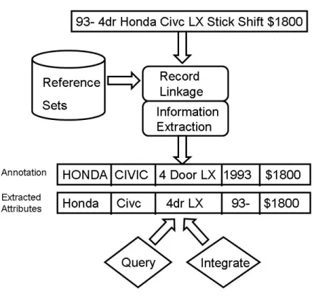
Next, we perform information extraction to extract the actual values in the post that match the schema elements defined by the reference set. This step is the information extraction step. During the information extraction step, the parts of the post are extracted that best match the attribute values from the reference set member chosen during the record linkage step. In this step we also extract attributes that are not easily represented by reference sets, such as prices or dates. Although we already have the schema and standardized attributes required to create a relational data set over the posts, we still extract the actual attributes embedded within the post so that we can more accurately learn to extract the attributes not represented by a reference set, such as prices and dates. While these attributes can be extracted using regular expressions, if we extract the actual attributes within the post we might be able to do so more accurately. For example, consider the “Ford 500” car. Without actually extracting the attributes within a post, we might extract “500” as a price, when it is actually a car name. Our overall approach is outlined in Figure 1.
Although we previously describe a similar approach to semantically annotating posts (Michelson & Knoblock, 2005), this paper extends that research by combining the annota-tion with our work on more scalable record matching (Michelson & Knoblock, 2006). Not only does this make the matching step for our annotation more scalable, it also demonstrates that our work on efficient record matching extends to our unique problem of matching posts, with embedded attributes, to structured, relational data. This paper also presents a more detailed description than our past work, including a more thorough evaluation of the pro-cedure than previously, using larger experimental data sets including a reference set that includes tens of thousands of records.
This article is organized as follows. We first describe our algorithm for aligning the posts to the best matching members of the reference set in Section 2. In particular, we show how this matching takes place, and how we efficiently generate candidate matches to make the matching procedure more scalable. In Section 3, we demonstrate how to exploit the matches to extract the attributes embedded within the post. We present some experiments in Section 4, validating our approaches to blocking, matching and information extraction for unstructured and ungrammatical text. We follow with a discussion of these results in Section 5 and then present related work in Section 6. We finish with some final thoughts and conclusions in Section 7.
Figure 1: Creating relational data from unstructured sources
2. Aligning Posts to a Reference Set
To exploit the reference set attributes to create relational data from the posts, the algo-rithm needs to first decide which member of the reference set best matches the post. This matching, known as record linkage (Fellegi & Sunter, 1969), provides the schema and at-tribute values necessary to query and integrate the unstructured and ungrammatical data source. Record linkage can be broken into two steps: generating candidate matches, called “blocking”; and then separating the true matches from these candidates in the “matching” step.
In our approach, the blocking generates candidate matches based on similarity methods over certain attributes from the reference set as they compare to the posts. For our cars example, the algorithm may determine that it can generate candidates by finding common tokens between the posts and the make attribute of the reference set. This step is detailed in Section 2.1 and is crucial in limiting the number of candidates matches we later examine during the matching step. After generating candidates, the algorithm generates a large set of features between each post and its candidate matches from the reference set. Using these features, the algorithm employs machine learning methods to separate the true matches from the false positives generated during blocking. This matching is detailed in Section 2.2.
2.1 Generating Candidates by Learning Blocking Schemes for Record Linkage
It is infeasible to compare each post to all of the members of a reference set. Therefore a preprocessing step generates candidate matches by comparing all the records between the sets using fast, approximate methods. This is called blocking because it can be thought of as partitioning the full cross product of record comparisons into mutually exclusive blocks (Newcombe, 1967). That is, to block on an attribute, first we sort or cluster the data sets by the attribute. Then we apply the comparison method to only a single member of a block. After blocking, the candidate matches are examined in detail to discover true matches.
There are two main goals of blocking. First, blocking should limit the number of can-didate matches, which limits the number of expensive, detailed comparisons needed during record linkage. Second, blocking should not exclude any true matches from the set of can-didate matches. This means there is a trade-off between finding all matching records and limiting the size of the candidate matches. So, the overall goal of blocking is to make the matching step more scalable, by limiting the number of comparisons it must make, while not hindering its accuracy by passing as many true matches to it as possible.
Most blocking is done using themulti-pass approach (Hernandez & Stolfo, 1998), which combines the candidates generated during independent runs. For example, with our cars data, we might make one pass over the data blocking on tokens in the car model, while another run might block using tokens of the make along with common tokens in the trim values. One can view the multi-pass approach as a rule in disjunctive normal form, where each conjunction in the rule defines each run, and the union of these rules combines the candidates generated during each run. Using our example, our rule might become ({ token-match, model} ∧({token-match, year})∪({token-match, make})). The effectiveness of the multi-pass approach hinges upon which methods and attributes are chosen in the conjunc-tions.
Note that each conjunction is a set of {method, attribute} pairs, and we do not make restrictions on which methods can be used. The set of methods could include full string metrics such as cosine similarity, simple common token matching as outlined above, or even state-of-the-art n-gram methods as shown in our experiments. The key for methods is not necessarily choosing the fastest (though we show how to account for the method speed below), but rather choosing the methods that will generate the smallest set of candidate matches that still cover the true positives, since it is the matching step that will consume the most time.
Therefore, a blocking scheme should include enough conjunctions to cover as many true matches as it can. For example, the first conjunct might not cover all of the true matches if the datasets being compared do not overlap in all of the years, so the second conjunct can cover the rest of the true matches. This is the same as adding more independent runs to the multi-pass approach.
However, since a blocking scheme includes as many conjunctions as it needs, these conjunctions should limit the number of candidates they generate. For example, the second conjunct is going to generate a lot of unnecessary candidates since it will return all records that share the same make. By adding more{method, attribute}pairs to a conjunction, we can limit the number of candidates it generates. For example, if we change ({token-match,
make}) to ({token-match, make} ∧ {token-match, trim}) we still cover new true matches, but we generate fewer additional candidates.
Therefore effective blocking schemes should learn conjunctions that minimize the false positives, but learn enough of these conjunctions to cover as many true matches as possi-ble. These two goals of blocking can be clearly defined by the Reduction Ratio and Pairs Completeness (Elfeky, Verykios, & Elmagarmid, 2002).
The Reduction Ratio (RR) quantifies how well the current blocking scheme minimizes the number of candidates. LetC be the number of candidate matches and N be the size of the cross product between both data sets.
RR= 1−C/N
It should be clear that adding more{method,attribute}pairs to a conjunction increases its RR, as when we changed ({token-match, zip}) to ({token-match, zip} ∧ {token-match, first name}).
Pairs Completeness (PC) measures the coverage of true positives, i.e., how many of the true matches are in the candidate set versus those in the entire set. IfSm is the number of
true matches in the candidate set, and Nm is the number of matches in the entire dataset,
then:
P C =Sm/Nm
Adding more disjuncts can increase our PC. For example, we added the second conjunc-tion to our example blocking scheme because the first did not cover all of the matches.
The blocking approach in this paper, “Blocking Scheme Learner” (BSL), learns effective blocking schemes in disjunctive normal form by maximizing the reduction ratio and pairs completeness. In this way, BSL tries to maximize the two goals of blocking. Previously we showed BSL aided the scalability of record linkage (Michelson & Knoblock, 2006), and this paper extends that idea by showing that it also can work in the case of matching posts to the reference set records.
The BSL algorithm uses a modified version of the Sequential Covering Algorithm (SCA), used to discover disjunctive sets of rules from labeled training data (Mitchell, 1997). In our case, SCA will learn disjunctive sets of conjunctions consisting of {method, attribute}
pairs. Basically, each call to LEARN-ONE-RULE generates a conjunction, and BSL keeps iterating over this call, covering the true matches left over after each iteration. This way SCA learns a full blocking scheme. The BSL algorithm is shown in Table 2.
There are two modifications to the classic SCA algorithm, which are shown in bold. First, BSL runs until there are no more examples left to cover, rather than stopping at some threshold. This ensures that we maximize the number of true matches generated as candidates by the final blocking rule (Pairs Completeness). Note that this might, in turn, yield a large number of candidates, hurting the Reduction Ratio. However, omitting true matches directly affects the accuracy of record linkage, and blocking is a preprocessing step for record linkage, so it is more important to cover as many true matches as possible. This way BSL fulfills one of the blocking goals: not eliminating true matches if possible. Second, if we learn a new conjunction (in the LEARN-ONE-RULE step) and our current blocking scheme has a rule that already contains the newly learned rule, then we can remove the rule containing the newly learned rule. This is an optimization that allows us to check rule containment as we go, rather than at the end.
Table 2: Modified Sequential Covering Algorithm SEQUENTIAL-COVERING(class, attributes, examples)
LearnedRules← {}
Rule←LEARN-ONE-RULE(class, attributes, examples) While examples left to cover, do
LearnedRules←LearnedRules∪Rule
Examples←Examples-{Examples covered by Rule}
Rule←LEARN-ONE-RULE(class, attributes, examples)
If Rule contains any previously learned rules, remove these contained rules.
Return LearnedRules
The rule containment is possible because we can guarantee that we learn less restrictive rules as we go. We can prove this guarantee as follows. Our proof is done by contradiction. Assume we have two attributesAandB, and a methodX. Also, assume that our previously learned rules contain the following conjunction, ({X, A}) and we currently learned the rule ({X, A}∧ {X, B}). That is, we assume our learned rules contains a rule that is less specific than the currently learned rule. If this were the case, then there must be at least one training example covered by ({X, A}∧ {X, B}) that is not covered by ({X,A}), since SCA dictates that we remove all examples covered by ({X, A}) when we learn it. Clearly, this cannot happen, since any examples covered by the more specific ({X, A}∧ {X, B}) would have been covered by ({X,A}) already and removed, which means we could not have learned the rule ({X, A}∧ {X, B}). Thus, we have a contradiction.
As we stated before, the two main goals of blocking are to minimize the size of the can-didate set, while not removing any true matches from this set. We have already mentioned how BSL maximizes the number of true positives in the candidate set and now we describe how BSL minimizes the overall size of the candidate set, which yields more scalable record linkage. To minimize the candidate set’s size, we learn as restrictive a conjunction as we can during each call toLEARN-ONE-RULE during the SCA. We define restrictive as mini-mizing the number of candidates generated, as long as a certain number of true matches are still covered. (Without this restriction, we could learn conjunctions that perfectly minimize the number of candidates: they simply return none.)
To do this, theLEARN-ONE-RULE step performs a general-to-specific beam search. It starts with an empty conjunction and at each step adds the {method, attribute}pair that yields the smallest set of candidates that still cover at least a set number of true matches. That is, we learn the conjunction that maximizes the Reduction Ratio, while at the same time covering a minimum value of Pairs Completeness. We use a beam search to allow for some backtracking, since the search is greedy. However, since the beam search goes from general-to-specific, we can ensure that the final rule is as restrictive as possible. The full LEARN-ONE-RULE is given in Table 3.
The constraint that a conjunction has a minimum PC ensures that the learned con-junction does not over-fit to the data. Without this restriction, it would be possible for LEARN-ONE-RULE to learn a conjunction that returns no candidates, uselessly producing an optimal RR.
The algorithm’s behavior is well defined for the minimum PC threshold. Consider, the case where the algorithm is learning as restrictive a rule as it can with the minimum coverage. In this case, the parameter ends up partitioning the space of the cross product of example records by the threshold amount. That is, if we set the threshold amount to 50% of the examples covered, the most restrictive first rule covers 50% of the examples. The next rule covers 50% of what is remaining, which is 25% of the examples. The next will cover 12.5% of the examples, etc. In this sense, the parameter is well defined. If we set the threshold high, we will learn fewer, less restrictive conjunctions, possibly limiting our RR, although this may increase PC slightly. If we set it lower, we cover more examples, but we need to learn more conjuncts. These newer conjuncts, in turn, may be subsumed by later conjuncts, so they will be a waste of time to learn. So, as long as this parameter is small enough, it should not affect the coverage of the final blocking scheme, and smaller than that just slows down the learning. We set this parameter to 50% for our experiments8.
Now we analyze the running time of BSL and we show how BSL can take into account the running time of different blocking methods, if need be. Assume that we havex(method,
attribute) pairs such as (token,f irst−name). Now, assume that our beam size isb, since we use general-to-specific beam-search in our Learn-One-Rule procedure. Also, for the time being, assume each (method, attribute) pair can generate its blocking candidates in O(1) time. (We relax this assumption later.) Each time we hit Learn-One-Rule within BSL, we will try all rules in the beam with all of the (attribute, method) pairs not in the current beam rules. So, in the worst case, this takes O(bx) each time, since for each (method, attribute) pair in the beam, we try it against all other (method, attribute) pairs. Now, in the worst case, each learned disjunct would only cover 1 training example, so our rule is a disjunction of all pairs x. Therefore, we run the Learn-One-Rule x times, resulting in a learning time of O(bx2). If we havee training examples, the full training time is O(ebx2), for BSL to learn the blocking scheme.
Now, while we assumed above that each (method, attribute) runs in O(1) time, this is clearly not the case, since there is a substantial amount of literature on blocking methods and 8. Setting this parameter lower than 50% had an insignificant effect on our results, and setting it much
higher, to 90%, only increased the PC by a small amount (if at all), while decreasing the RR.
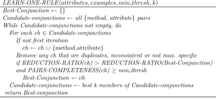
Table 3: Learning a conjunction of{method, attribute} pairs
LEARN-ONE-RULE(attributes, examples, min thresh, k)
Best-Conjunction← {}
Candidate-conjunctions←all{method, attribute}pairs While Candidate-conjunctions not empty, do
For each ch ∈Candidate-conjunctions If not first iteration
ch←ch∪ {method,attribute}
Remove any ch that are duplicates, inconsistent or not max. specific if REDUCTION-RATIO(ch)>REDUCTION-RATIO(Best-Conjunction) and PAIRS-COMPLETENESS(ch)≥min thresh
Best-Conjunction←ch
Candidate-conjunctions←best k members of Candidate-conjunctions return Best-conjunction
further the blocking times can vary significantly (Bilenko, Kamath, & Mooney, 2006). Let us define a functiontx(e) that represents how long it takes for a single (method, attribute)
pair in x to generate the e candidates in our training example. Using this notation, our Learn-One-Rule time becomesO(b(xtx(e))) (we runtx(e) time for each pair inx) and so our
full training time becomesO(eb(xtx(e))2). Clearly such a running time will be dominated
by the most expensive blocking methodology. Once a rule is learned, it is bounded by the time it takes to run the rule and (method, attribute) pairs involved, so it takesO(xtx(n)),
wheren is the number of records we are classifying.
From a practical standpoint, we can easily modify BSL to account for the time it takes certain blocking methods to generate their candidates. In the Learn-One-Rule step, we change the performance metric to reflect both Reduction Ratio and blocking time as a weighted average. That is, given Wrr as the weight for Reduction Ratio and Wb as the
weight for the blocking time, we modify Learn-One-Rule to maximize the performance of any disjunct based on this weighted average. Table 4 shows the modified version of Learn-One-Rule, and the changes are shown inbold.
Table 4: Learning a conjunction of {method, attribute} pairs using weights
LEARN-ONE-RULE(attributes, examples, min thresh, k)
Best-Conj ← {}
Candidate-conjunctions←all{method, attribute}pairs While Candidate-conjunctions not empty, do
For each ch∈Candidate-conjunctions If not first iteration
ch←ch∪ {method,attribute}
Remove any ch that are duplicates, inconsistent or not max. specific
SCORE(ch)=Wrr∗REDUCTION-RATIO(ch)+Wb∗BLOCK-TIME(ch)
SCORE(Best-Conj)=Wrr∗REDUCTION-RATIO(Best-conj)+Wb∗BLOCK-TIME(Best-conj) if SCORE(ch)>SCORE(Best-conj)
and PAIRS-COMPLETENESS(ch)≥min thresh Best-conj ←ch
Candidate-conjunctions←best k members of Candidate-conjunctions return Best-conj
Note that when we set Wb to 0, we are using the same version of Learn-One-Rule
as used throughout this paper, where we only consider the Reduction Ratio. Since our methods (token and n-gram match) are simple to compute, requiring more time to build the initial index than to do the candidate generation, we can safely set Wb to 0. Also,
making this trade-off of time versus reduction might not always be an appropriate decision. Although a method may be fast, if it does not sufficiently reduce the reduction ratio, then the time it takes the record linkage step might increase more than the time it would have taken to run the blocking using a method that provides a larger increase in reduction ratio. Since classification often takes much longer than candidate generation, the goal should be to minimize candidates (maximize reduction ratio), which in turn minimizes classification time. Further, the key insight of BSL is not only that we choose the blocking method, but more importantly that we choose the appropriate attributes to block on. In this sense, BSL is more like a feature selection algorithm than a blocking method. As we show in our
experiments, for blocking it is more important to pick the right attribute combinations, as BSL does, even using simple methods, than to do blocking using the most sophisticated methods.
We can easily extend our BSL algorithm to handle the case of matching posts to members of the reference set. This is a special case because the posts have all the attributes embedded within them while the reference set data is relational and structured into schema elements. To handle this special case, rather than matching attribute and method pairs across the data sources during our LEARN-ONE-RULE, we instead compare attribute and method pairs from the relational data to the entire post. This is a small change, showing that the same algorithm works well even in this special case.
Once we learn a good blocking scheme, we can now efficiently generate candidates from the post set to align to the reference set. This blocking step is essential for mapping large amounts of unstructured and ungrammatical data sources to larger and larger reference sets.
2.2 The Matching Step
From the set of candidates generated during blocking one can find the member of the reference set that best matches the current post. That is, one data source’s record (the post) must align to a record from the other data source (the reference set candidates). While the whole alignment procedure is referred to as record linkage (Fellegi & Sunter, 1969), we refer to finding the particular matches after blocking as the “matching step.”
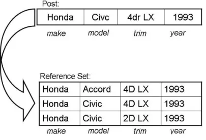
Figure 2: The traditional record linkage problem
However, the record linkage problem presented in this article differs from the “traditional” record linkage problem and is not well studied. Traditional record linkage matches a record from one data source to a record from another data source by relating their respective, decomposed attributes. For instance, using the second post from Table 1, and assuming decomposed attributes, the make from the post is compared to the make of the reference
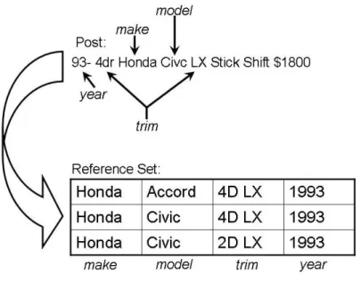
Figure 3: The problem of matching a post to the reference set
set. This is also done for themodels, thetrims, etc. The record from the reference set that best matches the post based on the similarities between the attributes would be considered the match. This is represented in Figure 2. Yet, the attributes of the posts are embedded within a single piece of text and not yet identified. This text is compared to the reference set, which is already decomposed into attributes and which does not have the extraneous tokens present in the post. Figure 3 depicts this problem. With this type of matching traditional record linkage approaches do not apply.
Instead, the matching step compares the post to all of the attributes of the reference set concatenated together. Since the post is compared to a whole record from the reference set (in the sense that it has all of the attributes), this comparison is at the “record level” and it approximately reflects how similar all of the embedded attributes of the post are to all of the attributes of the candidate match. This mimics the idea of traditional record linkage, that comparing all of the fields determines the similarity at the record level.
However, by using only the record level similarity it is possible for two candidates to generate the same record level similarity while differing on individual attributes. If one of these attributes is more discriminative than the other, there needs to be some way to reflect that. For example, consider Figure 4. In the figure, the two candidates share the same make and model. However, the first candidate shares the year while the second candidate shares the trim. Since both candidates share the same make and model, and both have another attribute in common, it is possible that they generate the same record level comparison. Yet, a trim on car, especially with a rare thing like a “Hatchback” should be more discriminative than sharing a year, since there are lots of cars with the same make, model and year, that differ only by the trim. This difference in individual attributes needs to be reflected.
To discriminate between attributes, the matching step borrows the idea from traditional record linkage that incorporating the individual comparisons between each attribute from
Figure 4: Two records with equal record level but different field level similarities
each data source is the best way to determine a match. That is, just the record level information is not enough to discriminate matches, field level comparisons must be exploited as well. To do “field level” comparisons the matching step compares the post to each individual attribute of the reference set.
These record and field level comparisons are represented by a vector of different simi-larity functions calledRL scores. By incorporating different similarity functions,RL scores reflects the different types of similarity that exist between text. Hence, for the record level comparison, the matching step generates the RL scores vector between the post and all of the attributes concatenated. To generate field level comparisons, the matching step calcu-lates theRL scores between the post and each of the individual attributes of the reference set. All of theseRL scores vectors are then stored in a vector calledVRL. Once populated,
VRL represents the record and field level similarities between a post and a member of the
reference set.
In the example reference set from Figure 3, the schema has 4 attributes <make, model, trim, year>. Assuming the current candidate is <“Honda”, “Civic”, “4D LX”, “1993”>, then theVRL looks like:
VRL=<RL scores(post, “Honda”),
RL scores(post, “Civic”), RL scores(post, “4D LX”), RL scores(post, “1993”),
RL scores(post, “Honda Civic 4D LX 1993”)>
VRL=<RL scores(post, attribute1), RL scores(post, attribute2), . . . ,
RL scores(post, attributen),
RL scores(post, attribute1 attribute2 . . . attributen)>
The RL scores vector is meant to include notions of the many ways that exist to define the similarity between the textual values of the data sources. It might be the case that one attribute differs from another in a few misplaced, missing or changed letters. This sort of similarity identifies two attributes that are similar, but misspelled, and is called “edit distance.” Another type of textual similarity looks at the tokens of the attributes and defines similarity based upon the number of tokens shared between the attributes. This “token level” similarity is not robust to spelling mistakes, but it puts no emphasis on the order of the tokens, whereas edit distance requires that the order of the tokens match in order for the attributes to be similar. Lastly, there are cases where one attribute may sound like another, even if they are both spelled differently, or one attribute may share a common root word with another attribute, which implies a “stemmed” similarity. These last two examples are neither token nor edit distance based similarities.
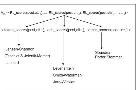
To capture all these different similarity types, the RL scores vector is built of three vec-tors that reflect the each of the different similarity types discussed above. Hence,RL scores is:
RL scores(post, attribute)=<token scores(post, attribute), edit scores(post, attribute), other scores(post, attribute)>
The vector token scores comprises three token level similarity scores. Two similarity scores included in this vector are based on the Jensen-Shannon distance, which defines similarities over probability distributions of the tokens. One uses a Dirichlet prior (Cohen, Ravikumar, & Feinberg, 2003) and the other smooths its token probabilities using a Jelenik-Mercer mixture model (Zhai & Lafferty, 2001). The last metric in the token scores vector is the Jaccard similarity.
With all of the scores included, the token scores vector takes the form: token scores(post, attribute)=<Jensen-Shannon-Dirichlet(post, attribute),
Jensen-Shannon-JM-Mixture(post, attribute), Jaccard(post, attribute)>
The vectoredit scoresconsists of the edit distance scores which are comparisons between strings at the character level defined by operations that turn one string into another. For instance, theedit scoresvector includes the Levenshtein distance (Levenshtein, 1966), which returns the minimum number of operations to turn string S into string T, and the Smith-Waterman distance (Smith & Smith-Waterman, 1981) which is an extension to the Levenshtein distance. The last score in the vector edit scores is the Jaro-Winkler similarity (Winkler & Thibaudeau, 1991), which is an extension of the Jaro metric (Jaro, 1989) used to find similar proper nouns. While not a strict edit-distance, because it does not regard operations of transformations, the Jaro-Winkler metric is a useful determinant of string similarity.
edit scores(post, attribute)=<Levenshtein(post, attribute), Smith-Waterman(post, attribute), Jaro-Winkler(post, attribute)>
All the similarities in theedit scores and token scores vector are defined in the Second-String package (Cohen et al., 2003) which was used for the experimental implementation as described in Section 4.
Lastly, the vector other scores captures the two types of similarity that did not fit into either the token level or edit distance similarity vector. This vector includes two types of string similarities. The first is the Soundex score between the post and the attribute. Soundex uses the phonetics of a token as a basis for determining the similarity. That is, misspelled words that sound the same will receive a high Soundex score for similarity. The other similarity is based upon the Porter stemming algorithm (Porter, 1980), which removes the suffixes from strings so that the root words can be compared for similarity. This helps alleviate possible errors introduced by the prefix assumption introduced by the Jaro-Winkler metric, since the stems are scored rather than the prefixes. Including both of these scores, theother scores vector becomes:
other scores(post, attribute)=<Porter-Stemmer(post, attribute), Soundex(post, attribute)>
Figure 5: The full vector of similarity scores used for record linkage
Figure 5 shows the full composition of VRL, with all the constituent similarity scores.
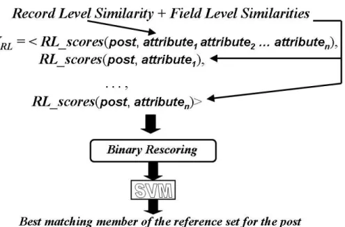
Once aVRL is constructed for each of the candidates, the matching step then performs
a binary rescoring on eachVRL to further help determine the best match amongst the
out the best candidate as much as possible. Because there might be a few candidates with similarly close values, and only one of them is a best match, the rescoring emphasizes the best match by downgrading the close matches so that they have the same element val-ues as the more obvious non-matches, while boosting the difference in score with the best candidate’s elements.
To rescore the vectors of candidate set C, the rescoring method iterates through the elements xi of allVRL∈C, and theVRL(s) that contain the maximum value forxi map this
xi to 1, while all of the otherVRL(s) mapxi to 0. Mathematically, the rescoring method is: ∀VRLj ∈C, j = 0...|C| ∀xi ∈VRLj, i= 0... VRLj f(xi, VRLj) = ( 1, xi= max(∀xt∈VRLs, VRLs ∈C, t=i, s= 0...|C|) 0, otherwise
For example, suppose C contains 2 candidates, VRL1 and VRL2:
VRL1 =<{.999,...,1.2},...,{0.45,...,0.22}>
VRL2 =<{.888,...,0.0},...,{0.65,...,0.22}>
After rescoring they become:
VRL1 =<{1,...,1},...,{0,...,1}>
VRL2 =<{0,...,0},...,{1,...,1}>
After rescoring, the matching step passes eachVRLto a Support Vector Machine (SVM)
(Joachims, 1999) trained to label them as matches or non-matches. The best match is the candidate that the SVM classifies as a match, with the maximally positive score for the decision function. If more than one candidate share the same maximum score from the decision function, then they are thrown out as matches. This enforces a strict 1-1 mapping between posts and members of the reference set. However, a 1-n relationship can be captured by relaxing this restriction. To do this the algorithm keeps either the first candidate with the maximal decision score, or chooses one randomly from the set of candidates with the maximum decision score.
Although we use SVMs in this paper to differentiate matches from non-matches, the algorithm is not strictly tied to this method. The main characteristics for our learning problem are that the feature vectors are sparse (because of the binary rescoring) and the concepts are dense (since many useful features may be needed and thus none should be pruned by feature selection). We also tried to use a Na¨ıve Bayes classifier for our matching task, but it was monumentally overwhelmed by the number of features and the number of training examples. Yet this is not to say that other methods that can deal with sparse feature vectors and dense concepts, such as online logistic regression or boosting, could not be used in place of SVM.
After the match for a post is found, the attributes of the matching reference set member are added as annotation to the post by including the values of the reference set attributes with tags that reflect the schema of the reference set. The overall matching algorithm is shown in Figure 6.
Figure 6: Our approach to matching posts to records from a reference set
In addition to providing a standardized set of values to query the posts, these standard-ized values allow for integration with outside sources because the values can be standardstandard-ized to canonical values. For instance, if we want to integrate our car classifieds with a safety ratings website, we can now easily join the sources across the attribute values. In this manner, by approaching annotation as a record linkage problem, we can create relational data from unstructured and ungrammatical data sources. However, to aid in the extraction of attributes not easily represented in reference sets, we perform information extraction on the posts as well.
3. Extracting Data from Posts
Although the record linkage step creates most of the relational data from the posts, there are still attributes we would like to extract from the post which are not easily represented by reference sets, which means the record linkage step can not be used for these attributes. Examples of such attributes are dates and prices. Although many of these such attributes can be extracted using simple techniques, such as regular expressions, we can make their extraction and annotation ever more accurate by using sophisticated information extraction. To motivate this idea, consider the Ford car model called the “500.” If we just used regular expressions, we might extract 500 as the price of the car, but this would not be the case. However, if we try to extract all of the attributes, including the model, then we would extract “500” as the model correctly. Furthermore, we might want to extract the actual attributes from a post, as they are, and our extraction algorithm allows this.
To perform extraction, the algorithm infuses information extraction with extra knowl-edge, rather than relying on possibly inconsistent characteristics. To garner this extra
knowledge, the approach exploits the idea of reference sets by using the attributes from the matching reference set member as a basis for identifying similar attributes in the post. Then, the algorithm can label these extracted values from the post with the schema from the reference set, thus adding annotation based on the extracted values.
In a broad sense, the algorithm has two parts. First we label each token with a possible attribute label or as “junk” to be ignored. After all the tokens in a post are labeled, we then clean each of the extracted labels. Figure 7 shows the whole procedure graphically, in detail, using the second post from Table 1. Each of the steps shown in this figure are described in detail below.
Figure 7: Extraction process for attributes
To begin the extraction process, the post is broken into tokens. Using the first post from Table 1 as an example, set of tokens becomes, {“93”, “civic”, “5speed”,...}. Each of these tokens is then scored against each attribute of the record from the reference set that was deemed the match.
To score the tokens, the extraction process builds a vector of scores,VIE. Like theVRL
vector of the matching step, VIE is composed of vectors which represent the similarities
between the token and the attributes of the reference set. However, the composition of VIE is slightly different from VRL. It contains no comparison to the concatenation of all
the attributes, and the vectors that compose VIE are different from those that compose
RL scores that composeVRL, except they do not contain thetoken scores component, since
each IE scores only uses one token from the post at a time. The RL scores vector:
RL scores(post, attribute)=<token scores(post, attribute), edit scores(post, attribute), other scores(post, attribute)>
becomes:
IE scores(token, attribute)=<edit scores(token, attribute), other scores(token, attribute)>
The other main difference between VIE and VRL is thatVIE contains a unique vector
that contains user defined functions, such as regular expressions, to capture attributes that are not easily represented by reference sets, such as prices or dates. These attribute types generally exhibit consistent characteristics that allow them to be extracted, and they are usually infeasible to represent in reference sets. This makes traditional extraction methods a good choice for these attributes. This vector is called common scores because the types of characteristics used to extract these attributes are “common” enough between to be used for extraction.
Using the first post of Table 1, assume the reference set match has the make “Honda,” the model “Civic” and the year “1993.” This means the matching tuple would be{“Honda”, “Civic”, “1993”}. This match generates the following VIE for the token “civic” of the post:
VIE=<common scores(“civic”),
IE scores(“civic”,“Honda”), IE scores(“civic”,“Civic”), IE scores(“civic”,“1993”)>
More generally, for a given token, VIE looks like:
VIE=<common scores(token),
IE scores(token, attribute1), IE scores(token, attribute2) . . . ,
IE scores(token, attributen)>
Each VIE is then passed to a structured SVM (Tsochantaridis, Joachims, Hofmann,
& Altun, 2005; Tsochantaridis, Hofmann, Joachims, & Altun, 2004) trained to give it an attribute type label, such as make, model, or price. Intuitively, similar attribute types should have similar VIE vectors. The makes should generally have high scores against the
make attribute of the reference set, and small scores against the other attributes. Further, structured SVMs are able to infer the extraction labels collectively, which helps in deciding between possible token labels. This makes the use of structured SVMs an ideal machine learning method for our task. Note that since eachVIE is not a member of a cluster where
the winner takes all, there is no binary rescoring.
Since there are many irrelevant tokens in the post that should not be annotated, the SVM learns that any VIE that does associate with a learned attribute type should be labeled as
“junk”, which can then be ignored. Without the benefits of a reference set, recognizing junk is difficult because the characteristics of the text in the posts are unreliable. For example, if extraction relies solely on capitalization and token location, the junk phrase “Great Deal” might be annotated as an attribute. Many traditional extraction systems that work in the domain of ungrammatical and unstructured text, such as addresses and bibliographies, assume that each token of the text must be classified as something, an assumption that cannot be made with posts.
Nonetheless, it is possible that a junk token will receive an incorrect class label. For example, if a junk token has enough matching letters, it might be labeled as atrim (since trims may only be a single letter or two). This leads to noisy tokens within the whole extractedtrim attribute. Therefore, labeling tokens individually gives an approximation of the data to be extracted.
The extraction approach can overcome the problems of generating noisy, labeled tokens by comparing the whole extracted field to its analogue reference set attribute. After all tokens from a post are processed, whole attributes are built and compared to the corre-sponding attributes from the reference set. This allows removal of the tokens that introduce noise in the extracted attribute.
The removal of noisy tokens from an extracted attribute starts with generating two baseline scores between the extracted attribute and the reference set attribute. One is a Jaccard similarity, to reflect the token level similarity between the two attributes. However, since there are many misspellings and such, an edit-distance based similarity metric, the Jaro-Winkler metric, is also used. These baselines demonstrate how accurately the system extracted/classified the tokens in isolation.
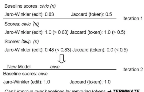
Using the first post of Table 1 as our ongoing example, assume the phrase “civic (ri)” was extracted as the model. This might occur if there is a car with the model Civic Rx, for instance. In isolation, the token “(ri)” could be the “Rx” of the model. Comparing this extracted car model to the reference attribute “Civic” generates a Jaccard similarity of 0.5 and a Jaro-Winkler score of 0.83. This is shown at the top of Figure 8.
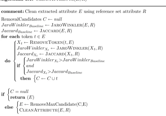
Next, the cleaning method goes through the extracted attribute, removing one token at a time and calculating new Jaccard and Jaro-Winkler similarities. If both new scores are higher than the baselines, that token becomes a removal candidate. After all the tokens are processed in this way, the removal candidate with the highest scores is removed, and the whole process is repeated. The scores derived using the removed token then become the new baseline to compare against. The process ends when there are no more tokens that yield improved scores over the baselines.
Shown as “Iteration 1” in Figure 8, the cleaning method finds that “(ri)” is a removal candidate since removing this token from the extracted car model yields a Jaccard score of 1.0 and a Jaro-Winkler score of 1.0, which are both higher than the baseline scores. Since it has the highest scores after trying each token in the iteration, it is removed and the baseline scores update. Then, since none of the remaining tokens provide improved scores (since there are none), the process terminates, yielding a more accurate attribute value. This is shown as “Iteration 2” in Figure 8. Note that this process would keep iterating, until no tokens can be removed that improve the scores over the baseline. The pseudocode for the algorithm is shown in Figure 9.
Figure 8: Improving extraction accuracy with reference set attributes
Note, however, that we do not limit the machine learning component of our extraction algorithm to SVMs. Instead, we claim that in some cases, reference sets can aid extraction in general, and to test this, in our architecture we can replace the SVM component with other methods. For example, in our extraction experiments we replace the SVM extractor with a Conditional Random Field (CRF) (Lafferty, McCallum, & Pereira, 2001) extractor that uses the VIE as features.
Therefore, the whole extraction process takes a token of the text, creates the VIE and
passes this to the machine-learning extractor which generates a label for the token. Then each field is cleaned and the extracted attribute is saved.
4. Results
The Phoebus system was built to experimentally validate our approach to building relational data from unstructured and ungrammatical data sources. Specifically, Phoebus tests the technique’s accuracy in both the record linkage and the extraction, and incorporates the BSL algorithm for learning and using blocking schemes. The experimental data, comes from three domains of posts: hotels,comic books, and cars.
The data from the hotel domain contains the attributes hotel name, hotel area, star rating, price and dates, which are extracted to test the extraction algorithm. This data comes from the Bidding For Travel website9 which is a forum where users share successful bids for Priceline on items such as airline tickets and hotel rates. The experimental data is limited to postings about hotel rates in Sacramento, San Diego and Pittsburgh, which compose a data set with 1125 posts, with 1028 of these posts having a match in the reference set. The reference set comes from the Bidding For Travel hotel guides, which are special
Algorithm 3.1: CleanAttribute(E, R)
comment:Clean extracted attribute E using reference set attributeR
RemovalCandidates C←null
J aroW inklerBaseline←JaroWinkler(E, R) J accardBaseline←Jaccard(E, R)
for each tokent∈E
do Xt←RemoveToken(t, E)
J aroW inklerXt ←JaroWinkler(Xt, R)
J accardXt ←Jaccard(Xt, R) if
J aroW inklerXt>J aroW inklerBaseline
and
J accardXt>J accardBaseline then nC←C∪t if ( C=null return (E) else ( E ←RemoveMaxCandidate(C,E) CleanAttribute(E, R)
Figure 9: Algorithm to clean an extracted attribute
posts listing all of the hotels ever posted about a given area. These special posts provide hotel names, hotel areas and star ratings, which are the reference set attributes. Therefore, these are the 3 attributes for which the standardized values are used, allowing us to treat these posts as a relational data set. This reference set contains 132 records.
The experimental data for the comic domain comes from posts for items for sale on eBay. To generate this data set, eBay was searched by the keywords “Incredible Hulk” and “Fantastic Four” in the comic books section of their website. (This returned some items that are not comics, such as t–shirts and some sets of comics not limited to those searched for, which makes the problem more difficult.) The returned records contain the attributes comic title, issue number, price, publisher, publication year and the description, which are extracted. (Note: the description is a few word description commonly associated with a comic book, such as 1st appearance the Rhino.) The total number of posts in this data set is 776, of which 697 have matches. Thecomic domain reference set uses data from the Comics Price Guide10, which lists all the Incredible Hulk and Fantastic Four comics. This reference set has the attributes title, issue number, description, and publisher and contains 918 records.
The cars data consists of posts made to Craigslist regarding cars for sale. This dataset consists of classifieds for cars from Los Angeles, San Francisco, Boston, New York, New 10. http://www.comicspriceguide.com/
Jersey and Chicago. There are a total of 2,568 posts in this data set, and each post contains a make, model, year, trim and price. The reference set for the Cars domain comes from the Edmunds11 car buying guide. From this data set we extracted the make, model, year and trim for all cars from 1990 to 2005, resulting in 20,076 records. There are 15,338 matches between the posts to Craigslist and the cars from Edmunds.
Unlike the hotels and comics domains, a strict 1-1 relationship between the post and reference set was not enforced in the cars domain. As described previously, Phoebus re-laxed the 1-1 relationship to form a 1-n relationship between the posts and the reference set. Sometimes the records do not contain enough attributes to discriminate a single best reference member. For instance, posts that contain just a model and a year might match a couple of reference set records that would differ on the trim attribute, but have the same make, model, and year. Yet, we can still use this make, model and year accurately for extraction. So, in this case, as mentioned previously, we pick one of the matches. This way, we exploit the attributes that we can from the reference set, since we have confidence in those.
For the experiments, posts in each domain are split into two folds, one for training and one for testing. This is usually called fold cross validation. However, in many cases two-fold cross validation results in using 50% of the data for training and 50% for testing. We believe that this is too much data to have to label, especially as data sets become large, so our experiments instead focus on using less training data. One set of experiments uses 30% of the posts for training and tests on the remaining 70%, and the second set of experiments uses just 10% of the posts to train, testing on the remaining 90%. We believe that training on small amounts of data, such as 10%, is an important empirical procedure since real world data sets are large and labeling 50% of such large data sets is time consuming and unrealistic. In fact, the size of the Cars domain prevented us from using 30% of the data for training, since the machine learning algorithms could not scale to the number of training tuples this would generate. So for the Cars domain we only run experiments training on 10% of the data. All experiments are performed 10 times, and the average results for these 10 trials are reported.
4.1 Record Linkage Results
In this subsection we report our record linkage results, broken down into separate discussions of our blocking results and our matching results.
4.1.1 Blocking Results
In order for the BSL algorithm to learn a blocking scheme, it must be provided with methods it can use to compare the attributes. For all domains and experiments we use two common methods. The first, which we call “token,” compares any matching token between the attributes. The second method, “ngram3,” considers any matching 3-grams between the attributes.
It is important to note that a comparison between BSL and other blockingmethods, such as the Canopies method (McCallum, Nigam, & Ungar, 2000) and Bigram indexing (Baxter, Christen, & Churches, 2003), is slightly misaligned because the algorithms solve different 11. www.edmunds.com
problems. Methods such as Bigram indexing are techniques that make theprocess of each blocking pass on an attribute more efficient. The goal of BSL, however, is to select which attribute combinationsshould be used for blocking as a whole, trying different attribute and method pairs. Nonetheless, we contend that it is more important to select the right attribute combinations, even using simple methods, than it is to use more sophisticated methods, but without insight as to which attributes might be useful. To test this hypothesis, we compare BSL using the token and 3-gram methods to Bigram indexing over all of the attributes. This is equivalent to forming a disjunction over all attributes using Bigram indexing as the method. We chose Bigram indexing in particular because it is designed to perform “fuzzy blocking” which seems necessary in the case of noisy post data. As stated previously (Baxter et al., 2003), we use a threshold of 0.3 for Bigram indexing, since that works the best. We also compare BSL to running a disjunction over all attributes using the simple token method only. In our results, we call this blocking rule “Disjunction.” This disjunction mirrors the idea of picking the simplest possible blocking method: namely using all attributes with a very simple method.
As stated previously, the two goals of blocking can be quantified by the Reduction Ratio (RR) and the Pairs Completeness (PC). Table 5 shows not only these values but also how many candidates were generated on average over the entire test set, comparing the three different approaches. Table 5 also shows how long it took each method to learn the rule and run the rule. Lastly, the column “Time match” shows how long the classifier needs to run given the number of candidates generated by the blocking scheme.
Table 6 shows a few example blocking schemes that the algorithm generated. For a comparison of the attributes BSL selected to the attributes picked manually for different domains where the data is structured the reader is pointed to our previous work on the topic (Michelson & Knoblock, 2006).
The results of Table 5 validate our idea that it is more important to pick the correct attributes to block on (using simple methods) than to use sophisticated methods without attention to the attributes. Comparing the BSL rule to the Bigram results, the combination of PC and RR is always better using BSL. Note that although in the Cars domain Bigram took significantly less time with the classifier due to its large RR, it did so because it only had a PC of 4%. In this case, Bigrams was not even covering 5% of the true matches.
Further, the BSL results are better than using the simplest method possible (the Disjuc-tion), especially in the cases where there are many records to test upon. As the number of records scales up, it becomes increasingly important to gain a good RR, while maintaining a good PC value as well. This savings is dramatically demonstrated by the Cars domain, where BSL outperformed the Disjunction in both PC and RR.
One surprising aspect of these results is how prevalent the token method is within all the domains. We expect that the ngram method would be used almost exclusively since there are many spelling mistakes within the posts. However, this is not the case. We hypothesize that the learning algorithm uses the token methods because they occur with more regularity across the posts than the common ngrams would since the spelling mistakes might vary quite differently across the posts. This suggests that there might be more regularity, in terms of what we can learn from the data, across the posts than we initially surmised.
Another interesting result is the poor reduction ratio of the Comic domain. This happens because most of the rules contain the disjunct that finds a common token within the comic
RR PC # Cands Time Learn (s) Time Run (s) Time match (s) Hotels (30%) BSL 81.56 99.79 19,153 69.25 24.05 60.93 Disjunction 67.02 99.82 34,262 0 12.49 109.00 Bigrams 61.35 72.77 40,151 0 1.2 127.74 Hotels (10%) BSL 84.47 99.07 20,742 37.67 31.87 65.99 Disjunction 66.91 99.82 44,202 0 15.676 140.62 Bigrams 60.71 90.39 52,492 0 1.57 167.00 Comics (30%) BSL 42.97 99.75 284,283 85.59 36.66 834.94 Disjunction 37.39 100.00 312,078 0 45.77 916.57 Bigrams 36.72 69.20 315,453 0 102.23 926.48 Comics (10%) BSL 42.97 99.74 365,454 34.26 35.65 1,073.34 Disjunction 37.33 100.00 401,541 0 52.183 1,179.32 Bigrams 36.75 88.41 405,283 0 131.34 1,190.31 Cars (10%) BSL 88.48 92.23 5,343,424 465.85 805.36 25,114.09 Disjunction 87.92 89.90 5,603,146 0 343.22 26.334.79 Bigrams 97.11 4.31 1,805,275 0 996.45 8,484.79
Table 5: Blocking results using the BSL algorithm (amount of data used for training shown in parentheses).
Hotels Domain (30%)
({hotel area,token} ∧ {hotel name,token} ∧ {star rating, token}) ∪({hotel name, ngram3}) Hotels Domain (10%)
({hotel area,token} ∧ {hotel name,token}) ∪ ({hotel name,ngram3}) Comic Domain (30%)
({title, token}) Comic Domain (10%)
({title, token}) ∪ ({issue number,token} ∧ {publisher,token} ∧ {title,ngram3}) Cars Domain (10%)
({make,token}) ∪({model,ngram3}) ∪({year,token} ∧ {make,ngram3}) Table 6: Some example blocking schemes learned for each of the domains.
title. This rule produces such a poor reduction ratio because the value for this attribute is the same across almost all reference set records. That is to say, when there are just a few unique values for the BSL algorithm to use for blocking, the reduction ratio will be small. In this domain, there are only two values for the comic title attribute, “Fantastic Four” and “Incredible Hulk.” So it makes sense that if blocking is done using the title attribute only, the reduction is about half, since blocking on the value “Fantastic Four” just gets rid of the “Incredible Hulk” comics. This points to an interesting limitation of the BSL algorithm. If there are not many distinct values for the different attribute and method pairs that BSL can use to learn from, then this lack of values cripples the performance of the reduction ratio. Intuitively though, this makes sense, since it is hard to distinguish good candidate matches from bad candidate matches if they share the same attribute values.
Another result worth mentioning is that in the Hotels domain we get a lower RR but the same PC when we use less training data. This happens because our BSL algorithm runs until it has no more examples to cover, so if those last few examples introduce a new disjunct that produces a lot of candidates, while only covering a few more true positives, then this would cause the RR to decrease, while keeping the PC at the same high rate. This is in fact what happens in this case. One way to curb this behavior would be to set some sort of stopping threshold for BSL, but as we said, maximizing the PC is the most important thing, so we choose not to do this. We want BSL to cover as many true positives as it can, even if that means losing a bit in the reduction.
In fact, we next test this notion explicitly. We set a threshold in the SCA such that after 95% of the training examples are covered, the algorithm stops and returns the learned blocking scheme. This helps to avoid the situation where BSL learns a very general conjunc-tion, solely to cover the last few remaining training examples. When that happens, BSL might end up lowering the RR, at the expense of covering just those last training examples, because the rule learned to cover those last examples is overly general and returns too many candidate matches.
Domain Record Linkage RR PC F-Measure Hotels Domain No Thresh (30%) 90.63 81.56 99.79 95% Thresh (30%) 90.63 87.63 97.66 Comic Domain No Thresh (30%) 91.30 42.97 99.75 95% Thresh (30%) 91.47 42.97 99.69 Cars Domain No Thresh (10%) 77.04 88.48 92.23 95% Thresh (10%) 67.14 92.67 83.95
Table 7: A comparison of BSL covering all training examples, and covering 95% of the training examples
Table 7 shows that when we use a threshold in the Hotels and Cars domain we see a statistically significant drop in Pairs Completeness with a statistically significant increase in Reduction Ratio.12 This is expected behavior since the threshold causes BSL to kick out of SCA before it can cover the last few training examples, which in turn allows BSL to retain a rule with high RR, but lower PC. However, when we look at the record linkage results, we see that this threshold does in fact have a large effect.13 Although there is no statistically significant difference in the F-measure for record linkage in the Hotels domain, the difference in Cars domain is dramatic. When we use a threshold, the candidates not discovered by the rule generated when using the threshold have an effect of 10% on the final F-measure match results.14 Therefore, since the F-measure results differ by so much, we conclude that it is worthwhile to maximize PC when learning rules with BSL, even if the RR may decrease. That is to say, even in the presence of noise, which in turn may lead to overly generic blocking schemes, BSL should try to maximize the true matches it covers, because avoiding even the most difficult cases to cover may affect the matching results. As we see in Table 7, this is especially true in the Cars domain where matching is much more difficult than in the Hotels domain.
Interestingly, in the Comic domain we do not see a statistically significant difference in the RR and PC. This is because across trials we almost always learn the same rule whether we use a threshold or not, and this rule covers enough training examples that the threshold is not hit. Further, there is no statistically significant change in the F-measure record linkage results for this domain. This is expected since BSL would generate the same candidate matches, whether it uses the threshold or not, since in both cases it almost always learns the same blocking rules.
Our results using BSL are encouraging because they show that the algorithm also works for blocking when matching unstructured and ungrammatical text to a relational data source. This means the algorithm works in this special case too, not just the case of traditional record linkage where we are matching one structured source to another. This means our overall algorithm for semantic annotation is much more scalable because we are using fewer candidate matches than in our previous work (Michelson & Knoblock, 2005).
4.1.2 Matching Results
Since this alignment approach hinges on leveraging reference sets, it becomes necessary to show the matching step performs well. To measure this accuracy, the experiments employ the usual record linkage statistics:
P recision= #CorrectM atches #T otalM atchesM ade Recall= #CorrectM atches
#P ossibleM atches
12. Bold means statistically significant using a two-tailed t-test withαset to 0.05
13. Please see subsection 4.1.2 for a description of the record linkage experiments and results.
14. Much of this difference is attributed to the non-threshold version of the algorithm learning a final predicate that includes the make attribute by itself, which the version with a threshold does not learn. Since each make attribute value covers many records, it generates many candidates which results in increasing PC while reducing RR.