Selection for Ensemble Classifiers
Rakkrit Duangsoithong and Terry Windeatt
Abstract PC and TPDA algorithms are robust and well known prototype algorithms, incorporating constraint-based approaches for causal discovery. However, both al-gorithms cannot scale up to deal with high dimensional data, that is more than few hundred features. This chapter presents hybrid correlation and causal feature se-lection for ensemble classifiers to deal with this problem. Redundant features are removed by correlation-based feature selection and then irrelevant features are elim-inated by causal feature selection. The number of elimelim-inated features, accuracy, the area under the receiver operating characteristic curve (AUC) and false negative rate (FNR) of proposed algorithms are compared with correlation-based feature selec-tion (FCBF and CFS) and causal based feature selecselec-tion algorithms (PC, TPDA, GS, IAMB).
1 Introduction
With rapid development of computer and information technology that can improve a large number of applications such as web text mining, intrusion detection, biomedi-cal informatics, gene selection in micro array data, medibiomedi-cal data mining, and clinibiomedi-cal decision support systems, many information databases have been created. However, in some applications especially in medical area, data may contain hundreds to thou-sands of features with small sample size. A consequence of this problem is increased complexity that leads to degradation in efficiency and accuracy by curse of
dimen-Rakkrit Duangsoithong
Centre for Vision, Speech and Signal Processing, University of Surrey, Guildford, United Kingdom GU2 7XHe-mail: [email protected]
Terry Windeatt
Centre for Vision, Speech and Signal Processing, University of Surrey, Guildford, United Kingdom GU2 7XH e-mail: [email protected]
sionality and over-fitting. The resulting classifier works very well with training data but very poorly on test data.
To overcome this high dimensional feature spaces degradation problem, num-ber of features should be reduced. Basically, there are two methods to reduce the dimension: feature extraction and feature selection. Feature extraction transforms or projects original features to fewer dimensions without using prior knowledge. Nevertheless, it lacks comprehensibility and uses all original features which may be impractical in large feature spaces. On the other hand, feature selection selects optimal feature subsets from original features by removing irrelevant and redundant features. It has the ability to reduce over-fitting, increase classification accuracy, reduce complexity, speed of computation and improve comprehensibility by pre-serving original semantic of datasets. Normally, clinicians prefer feature selection because of its understandability and user acceptance.
Feature selection is an important pre-processing step to reduce feature dimen-sions for classification and generally, can be divided into four categories [15],[18],[9]. Filter method is independent from learning method and uses measurement tech-niques such as correlation and distance measurement to find a good subset from entire set of features. Wrapper method uses pre-determined learning algorithm to evaluate selected feature subsets that are optimum for the learning process. Hybrid method combines advantage of both Filter and Wrapper method together. It evalu-ates features by using an independent measure to find the best subset and then uses a learning algorithm to find the final best subset. Finally, Embedded method interacts with learning algorithm but it is more efficient than Wrapper method because the filter algorithm has been built with the classifier.
As has been illustrated by Liu and Yu [15], feature selection has four basic pro-cesses: Subset generation, subset evaluation, stopping criterion and subset valida-tion. Subset generation produces candidate subset by complete (exhaustive), se-quential (heuristic) or random search with three directions: forward (adding feature to selected subset that begin with empty set), backward (eliminate features from se-lected subset that begins with full original set) and bidirectional (both adding and removing features). After that, the candidate subset is evaluated based on criteria such as distance, dependency and information gain and consistency measurement. The process will stop when it reaches the stopping criterion. Finally, the selected subset is validated with validation data.
Feature selection does not usually take causal discovery into account. However, in some cases such as when training and testing dataset do not conform to i.i.d. as-sumption, testing distribution is shifted from manipulation by external agent, causal discovery can provide some benefits for feature selection under these uncertainty conditions. Causal relationships are usually uncovered by Bayesian Networks (BNs) which consist of a direct acyclic graph (DAG) that represents dependencies and in-dependencies between variable and joint probability distribution among a set of vari-ables [1]. It also can learn underlying data structure, provide better understanding of the data generation process and better accuracy and robustness under uncertainty [10].
An ensemble classifier or multiple classifier system (MCS) is another well-known technique to improve system accuracy [24]. Ensembles combine multiple base classifiers to learn a target function. It has ability to increase accuracy by com-bining output of multiple experts to reduce bias and variance [3], improve efficiency by decomposing complex problem into multiple sub problems and improve relia-bility by reducing uncertainty. To increase accuracy, each classifier in the ensemble should be diverse or unique such as starting with different input, initial weight, ran-dom features or ranran-dom classes [23].
Generally, the number of features in feature selection analysis can be divided into three categories: small scale (the number of features is less than 19), medium scale (the number of features is between 20 and 49) and large scale (the number of features is equal or higher than 50 features) [12],[27]. The main purpose of this research is to find methods that can scale up to deal with hundreds or thousands of features.
The main objective of this chapter is to find approaches that enable PC and TPDA algorithms to deal with high dimensional data. We propose hybrid correlation and causal feature selection for ensemble classifiers and compare number of eliminated features, average percent accuracy, the area under the receiver operating character-istic curve (AUC) and false negative rate (FNR).
The structure of the chapter is the following: related research is briefly described in Section 2. Section 3 explains theoretical approach of feature selection, causal dis-covery and ensemble classifiers. The dataset and evaluation procedure are described in Section 4. Experimental results are presented in Section 5 and are discussed in Section 6. Finally, Conclusion is summarized in Section 7.
2 Related Research
Feature selection and ensemble classification have received attention from many researchers in the areas of statistics, machine learning, neural networks and data mining for many years. Initially, most researchers focused only on removing ir-relevant features such as ReliefF [25], FOCUS [2] and Correlation-based Feature Selection(CFS) [8]. Recently, in Yu and Liu (2004) [26], Fast Correlation-Based Filter (FCBF) algorithm was proposed to remove both irrelevant and redundant fea-tures by using Symmetrical Uncertainty (SU) measurement and was successful for reducing high dimensional features while maintaining high accuracy.
In the past few years, learning Bayesian Networks (BNs) from observation data has received increasing attention from researchers for many applications such as decision support system, information retrieval, natural language processing, fea-ture selection and gene expression data analysis [21],[22]. The category of BNs can be divided into three approaches: Search-and-Score, Constraint-Based and Hy-brid approaches [21],[22]. In Search-and-Score approach, BNs search all possible structures to find the one that provides the maximum score. The standard Scoring functions that normally used in BNs are Bayesian Dirichlet (BDeu), Bayesian
Infor-mation Criterion (BIC), Akaike InforInfor-mation Criterion (AIC), Minimum Description Length (MDL) and K2 scoring function [21]. The second approach, Constraint-Based, uses test of conditional dependencies and independencies from the data by estimation using G2statistic test or mutual information, etc. This approach defines structure and orientation from results of the tests based on some assumptions that these tests are accurate. Finally, Hybrid approach uses Constraint-Based approach for conditional independence test (CI test) and then identifies the network that max-imizes a scoring function by using Search-and-Score approach [22].
Constraint-Based algorithms are computationally effective and suitable for high dimensional feature spaces. PC algorithm [19], is a pioneer, prototype and well-known global algorithm of Constraint-Based approach for causal discovery. Three Phase Dependency Analysis (TPDA or PowerConstructor) [6] is another global Constraint-Based algorithm that uses mutual information to search and test for CI test instead of using G2Statistics test as in PC algorithm. However, both PC and TPDA algorithm use global search to learn from the complete network and can not scale up to more than few hundred features (they can deal with 100 and 255 features for PC and TPDA, respectively) [20]. Sparse Candidate algorithm (SC) [7] is one of the prototype BNs algorithm that can deal with several hundreds of features by us-ing local candidate set. Nevertheless, SC algorithm has some disadvantages, it may not identify true set of parents and users have to find appropriate k parameter of SC algorithm [21].
Recently, many Markov Blanket-based algorithms for causal discovery have been studied extensively and they have ability to deal with high dimensional feature spaces such as MMMB, IAMB [20] and HITON [1] algorithms. HITON is a state-of-the-art algorithm that has ability to deal with thousands of features and can be used as an effective feature selection method in high dimensional spaces. However, HITON and all other MB-based algorithms may not specify features in Markov Blanket for desired classes or target (MB(T)) when the data is not faithful [5].
3 Theoretical Approach
In our research, hybrid algorithm of correlation and causal feature selection is com-pared with Fast Correlation-Based Filter (FCBF), Correlation-based Feature Se-lection with Sequential Forward Floating Search direction (CFS+SFFS), and with causal feature selection algorithms (PC, TPDA, GS and IAMB) using Bagging (de-scribed in Section 3.4).
3.1 Feature Selection Algorithms
3.1.1 Fast Correlation-Based Filter (FCBF)
FCBF [26] algorithm is a correlation-based filter which has two stages: relevance analysis and redundancy analysis.
Relevance Analysis
Normally, correlation is widely used to analyze relevance in linear system and can be measured by linear correlation coefficience.
r=p ∑i(xi−xi)(yi−yi)
∑i(xi−xi)2
p
∑i(yi−yi)2
(1) However, most systems in real world applications are non-linear. Correlation in non-linear systems can be measured by using Symmetrical Uncertainty (SU).
SU(X,Y) =2 h IG(X|Y) H(X) +H(Y) i (2) IG(X|Y) =H(X)−H(X|Y) (3) H(X) =−
∑
i P(xi)log2P(xi) (4)here IG(X|Y)is the Information Gain of X after observing variable Y . H(X)and H(Y)are the entropy of variable X and Y , respectively. P(xi)is the probability of variable x.
SU is the modified version of Information Gain that has range between 0 and 1. FCBF removes irrelevant features by ranking correlation (SU) between feature and class. If SU between feature and class equal to 1, it means that this feature is completely related to that class. On the other hand, if SU is equal to 0, the features are irrelevant to this class.
Redundancy analysis
Redundant features can be defined from meaning of predominant feature and approximate Markov Blanket. In Yu and Liu (2004) [26], a feature is predomi-nant (both relevant and non redundant feature) if it does not have any approximate Markov Blanket in the current set.
Approximate Markov Blanket: For two relevant features Fi and Fj (i6= j), Fj forms an approximate Markov Blanket for Fiif
where SUi,cis a correlation between any feature and the class. SUi,jis a
correla-tion between any pair of feature Fiand Fj(i6=j).
3.1.2 Correlation-based Feature Selection (CFS).
CFS [8] is one of well-known techniques to rank the relevance of features by mea-suring correlation between features and classes and between features and other fea-tures.
Given number of features k and classes c, CFS defined relevance of features subset by using Pearson’s correlation equation
Merits=
krkc
p
k+ (k−1)rkk
(6) where Meritsis relevance of feature subset, rkcis the average linear correlation coefficient between these features and classes and rkkis the average linear correla-tion coefficient between different features.
Normally, CFS adds (forward selection) or deletes (backward selection) one fea-ture at a time, however, in this research, we used Sequential Forward Floating Search (SFFS) [17] as the search direction because of its powerful search scheme which is very fast and does not require any tuning parameters.
Sequential Forward Floating Search (SFFS). SFFS [17] is one of a classic heuristic searching method. It is a variation of bidirectional search and sequential forward search (SFS) that has dominant direction on forward search. SFFS removes features (backward elimination) after adding features (forward selection). The num-ber of forward and backward step is not fixed but dynamically controlled depending on the criterion of the selected subset and therefore, no parameter setting is required.
3.2 Causal Discovery Algorithm
In this chapter, two standard constraint-based approaches (PC and TPDA) and two Markov Blanket based algorithms (GS, IAMB) are used as causal feature selection methods. In the final output of the causal graph from each algorithm, the uncon-nected features to classes will be considered as eliminated features.
3.2.1 PC Algorithm
PC algorithm [19],[10] is the prototype of constraint-based algorithm. It consists of two phases: Edge Detection and Edge Orientation.
Edge Detection: the algorithm determines directed edge by using conditionally independent condition. The algorithm starts with:
i) Undirected edge with fully connected graph.
ii) Remove a share direct edge between A and B (A−B) iff there is a subset F of features that can present conditional independence(A,B|F).
Edge Orientation: The algorithm discovers V-Structure A−B−C in which A−C is missing.
i) If there are direct edges between A−B and B−C but not A−C, then orient edge A→B←C until no more possible orientation.
ii) If there is a path A→B−C and A−C is missing, then A→B→C. iii) If there is orientation A→B→...→C and A−C then orient A→C.
3.2.2 Three Phase Dependency Analysis Algorithm (TPDA)
TPDA or PowerConstructor algorithm [6] has three phases: drafting, thickening and thinning phases.
Drafting phase: mutual information of each pair of nodes is calculated and used to create a graph without loop.
Thickening phase: edge will be added when that pair of nodes can not be d-separated. (node A and B are d-separated by node C iff node C blocks every path from node A to node B [21].) The output of this phase is called an independence map (I-map).
Thinning phase: The edge of I-map will be removed in thinning phase, if two nodes of the edge can be d-separated and the final output is defined as a perfect map [6].
3.2.3 Grow-Shrink algorithm (GS)
GS [16] algorithm consists of two phases; forward and backward phases.
Forward phase: GS statistically ranks features by using the strength of associ-ation with target or class (T) given empty set. After that the next ordering feature which is not conditionally independent from class T given current Markov Blanket (CMB) will added into CMB.
Backward phase: Identify false positive nodes and remove them from CMB. At this stage, CMB=MB(T). Finally, a feature X will be removed from CMB one-by-one if that feature X is independent of class T given the remaining CMB.
3.2.4 Incremental Association Markov Blanket Algorithm (IAMB)
IAMB [20] is one of Markov Blanket detection algorithms using forward selection followed by removing false positive node. IAMB has two phases, forward and back-ward.
Forward phase: In forward selection phase, the algorithm starts with empty set in CMB, then adding features which maximizes a heuristic function f(X ; T|CMB). A feature member in MB(T) will not return zero value of this function.
Backward phase: False positive nodes will be removed from CMB by using con-dition independent testing of class T given the rest CMB.
3.3 Feature Selection Analysis
3.3.1 Correlation-based Redundancy and Relevance Analysis
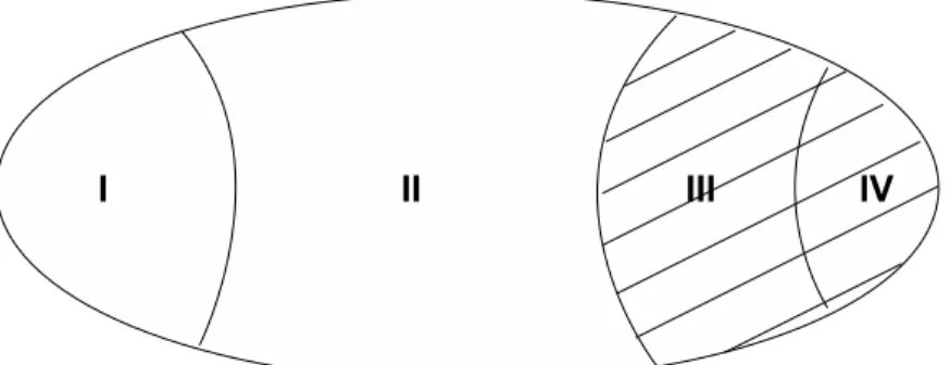
The concept of selecting optimal subset from whole features is presented in Figure 1 [26] where I is irrelevant feature, II is weakly relevant and redundant feature, III is weakly relevant but non redundant feature. IV is strongly relevant feature and III+IV are optimal subset.
Fig. 1 Optimal Subset
Optimal subset should include all strongly relevant features, subset of weakly relevant features that have no redundancy and none of the irrelevant features.
In 2004, Yu and Liu [26] proposed FCBF algorithm to remove both redundant and irrelevant features.
1) Redundancy: A feature is redundant if it has approximate Markov Blanket (SUj,c≥SUi,cand SUi,j≥SUi,c).
2) Irrelevance: A feature is irrelevant if SU between feature and class is zero. 3) Relevance: A feature is relevant if SU between feature and class is more than zero but less than one.
4) Strong relevance: A feature is strongly relevant if SU between feature and class is equal to one.
3.3.2 Causal-based Relevance Analysis
In Guyon [10], the notion of Markov Blanket is defined in term of Kohavi-John feature relevance:
1) Irrelevance: A feature is irrelevant if it is disconnected from graph (condi-tional independence).
2) Relevance: A feature is relevant if it has connected path to class (target). 3) Strong relevance: A feature is strongly relevant if it is Markov Blanket of class.
3.3.3 Hybrid Correlation-Based Redundancy Causal-Based Relevance Analysis
According to figure 1 and the above analysis, optimal subset consists of strongly relevant features and weakly relevant features that do not contain redundant and irrelevant features. Therefore, we propose a new analysis for Hybrid Correlation-Based Relevance Causal-Correlation-Based Redundancy Analysis as follows:
1) Redundancy: A feature is redundant if it has approximate Markov Blanket. 2) Irrelevance: A feature is irrelevant if it is disconnected from the graph (con-ditional independence).
3) Relevance: A feature is relevant if it has connected path to the target (class). 4) Strong relevance: A feature is strongly relevant if it is Markov Blanket of the target (class).
Table 1 shows the summary analysis of redundancy and relevancy analysis for correlation-based [26], causal-based [10] and proposed hybrid correlation and causal feature selection. Markov Blanket (MB(T)) of target or class (T) is the min-imal set of conditional features that all other features are probabilistically indepen-dent of T. It consists of the set of parents, children and spouses of T.
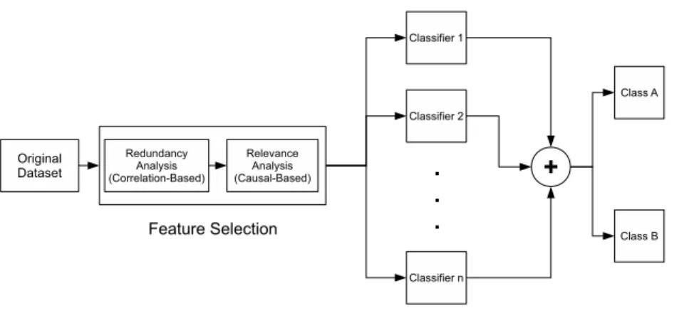
Figure 2 presents the proposed system block diagram. Redundant features are re-moved by correlation-based feature selection and irrelevant features are eliminated by causal-based feature selection. After that, selected features are passed through
Table 1 Summary analysis of correlation, causal and proposed hybrid correlation and causal fea-ture selection for redundancy and relevance analysis.
Relation Correlation-Based Causal-Based Hybrid algorithm
Strongly relevant SUi,c=1 Features in Features in
Markov Blanket Markov Blanket
Weakly relevant does not has approximate connected connected
without redundant features Markov Blanket to classes to classes
Weakly relevant has approximate connected has approximate
with redundant features Markov Blanket to classes Markov Blanket
Irrelevant SUi,c=0 disconnected disconnected
to classes to classes
ensemble classifier for training and predicting output.
3.4 Ensemble Classifier
Bagging [4] or Bootstrap aggregating is one of the earliest, simplest and most pop-ular methods for ensemble based classifiers. Bagging uses Bootstrap that randomly samples with replacement and combines with majority vote. The selected data is divided to m bootstrap replicates and randomly sampled with replacement. Each bootstrap replicate contains, on average, 63.2 % of the original dataset. Final out-put will be selected from majority vote of all classifiers of each bootstrap replicate. Bootstrap is the most well-known strategy for injecting randomness to improve gen-eralization performance in multiple classifier systems and provides out-of-bootstrap estimate for selecting classifier parameters [24]. Randomness is desirable since it increases diversity among the base classifiers, which is known to be a necessary condition for improved performance. However, there is an inevitable trade-off be-tween accuracy and diversity known as the accuracy/diversity dilemma [24].
Nevertheless, in causal discovery, there are some disadvantages for BNs learning using Bagging. Bootstrap method can add many extra edges in graphical model due to more complexity especially in high dimensional features with limited dataset [13]. Moreover, distribution from bootstrap dataset may not satisfy Markov Blanket condition and faithfulness condition [14].
3.5 Pseudo-code: Hybrid Correlation and Causal Feature Selection
for Ensemble Classifiers algorithm
Goal : To find optimal subset features for ensemble classifiers by using correlation and causal discovery.
3.5.1 Eliminate redundant features by using correlation
⋄Input: Training set (each pattern having features{f1,f2, ...,fn}and class{C})
⋄Output: Selected features without redundant features{S1}
•Calculate SU between features and between feature and classes, find and remove redundant features using approximate Markov Blanket.
for i=1 to n−1, j=i+1
fi= first feature, fj= next feature calculate SUi,j, SUi,cand SUj,c
if SUi,c≥SUj,cand SUi,j≥SUj,c
then remove fj
else Append fjto output selected features list{S1}
3.5.2 Remove irrelevant features by using causal discovery ⋄Input: Selected features without redundant features.{S1}
⋄Output: Optimal features without redundant and irrelevant features.{S2}
•Find constructor and direction of graph by using causal discovery algorithm. (PC, TPDA, GS, IAMB or other causal discovery algorithm)
•Remove irrelevant features which are disconnected from class. - PC Algorithm
Edge Detection: using conditionally independent condition.
Starts with completely connected graph G. i=−1
repeat i=i+1 repeat
- Select and order pair of features (nodes) A,B in graph G. - Select adjacent (neighborhood) feature F of A with size i - if there exists a feature F that presents conditional independence
(A,B|F), delete direct edge between A and B. until all ordered pairs of feature F have been tested. until all adjacent features have size smaller than i.
Edge Orientation: directed edges using following rules;
•If there are direct edges between A−B and B−C but not A−C, then orient edge A→B←C until no more possible orientation.
•If there is a path A→B−C and A−C is missing, then A→B→C. •If there is orientation A→B→...→C and A−C then orient A→C.
- Three Phase Dependency Analysis Algorithm (TPDA). Drafting phase
•calculated mutual information (MI) of each pair of features. •create a graph without loop using MI.
Thickening phase
•add edge when that pair of nodes can not be d-separated. •the output of this phase is called an independence map (I-map). Thinning phase
•remove the edge of I-map, if two nodes of the edge can be d-separated. •the final output is defined as a perfect map.
3.5.3 Ensemble classifiers using Bagging algorithm .⋄Input:
•Optimal features without redundant and irrelevant features{S2}
•Number of bootstrap sample (m) (number of iterations) with 100 percentage set-ting from original data
•Classifier or Inducer function (I)
for i=1 to m
{S′2}= bootstrap sample from{S2}
Ci=I{S′2}//(class output of each bootstrap replicate) end for
⋄Output:
•ensemble classifiers prediction based on majority vote (C∗(x)) •y is one of the class of total Y classes
•count majority vote class from all output of bootstrap replicates C∗(x) =argmaxy∈Y ∑i:Ci(x)=y1
4 Experimental Setup
4.1 Dataset
The datasets used in this experiment were taken from Causality Challenge [11] and details of each dataset are shown as follows;
LUCAS (LUng CAncer Simple set) dataset is toy data generated artificially by causal Bayesian networks with binary features. Both dataset are modelling a medi-cal application for the diagnosis, prevention and cure of lung cancer. Lucas has 11 features with binary classes and 2000 samples.
LUCAP (LUng CAncer set with Probes) is LUCAS dataset with probes which are generated from some functions plus some noise of subsets of the real variables. LUCAP has 143 features, 2000 samples and binary classes.
REGED (REsimulationed Gene Expression Dataset) is dataset that simulated model from real human lung cancer micro array gene expression data. The target to simulate this data is to find genes which could be responsible of lung cancer. It contains 500 examples with 999 features and binary classes.
CINA (Census Is Not Adult) dataset derived from Census dataset from UCI Ma-chine learning repository. The goal of dataset is to uncover the socio-economic fac-tors affecting high income. It has 132 features which contains 14 original features and distracter features which are artificially generated features that are not causes of the classes, 16,033 examples and binary classes.
SIDO (SImple Drug Operation mechanisms) has 4,932 features, 12678 samples and 2 classes. Sido dataset consists of molecules descriptors that have been tested against the AIDS HIV virus and probes which artificially generated features that are not causes of the target.
Due to large number of samples and limitation of computer memory during val-idation in CINA and SIDO datasets, the number of samples of both dataset are re-duced to 10 percent (1603 and 1264 samples, respectively) from the original dataset.
4.2 Evaluation
To evaluate feature selection process we use four widely used classifiers: Naive-Bayes(NB), Multilayer Perceptron (MLP), Support Vector Machines (SVM) and Decision Trees (DT). The parameters of each classifier were chosen as follows. MLP has one hidden layer with 16 hidden nodes, learning rate 0.2, momentum 0.3, 500 iterations and uses backpropagation algorithm with sigmoid transfer function. SVM uses polynomial kernel with exponent 2 and the regularization value set to 0.7. DT uses pruned C4.5 algorithm. The number of classifiers in Bagging is var-ied from 1, 5, 10, 25 to 50 classifiers. The threshold value of FCBF algorithm in our research is set at zero for LUCAS, REGED, CINA, SIDO and 0.14 for LUCAP dataset, respectively.
The classifier results were validated by 10 fold cross validation with 10 rep-etitions for each experiment and evaluated by average percent of test set accuracy, False Negative Rate (FNR) and area under the receiver operating characteristic curve (AUC).
In two-class prediction, there are four possible results of classification as shown in table 2.
Table 2 Four possible outcomes from two-classes prediction.
Predicted Class
Positive Negative
Actual Positive True Positive (TP) False Negative (FN)
Accuracy Accuracy of classification measurement can be calculated from the ratio between number of correct predictions (True Positive(TN) and True Negative (TN)) and total number of all possible outcomes (TP,TN,FP and FN).
Accuracy=h T P+T N
T P+FP+FN+T N i
(7)
The area under the receiver operating characteristic curve (AUC) AUC is a graph of true positive against false positive. AUC has value between 0 and 1. The AUC value of 1 represents a perfect classifier performance while AUC lower than 0.5 represents a poor prediction.
False Negative Rate (FNR) For medical dataset, FNR is the ratio of number of patient with negative prediction (False Negative (FN)) per number with disease condition (FN and TP).
FNR=h FN
FN+T P i
(8)
For causal feature selection, PC algorithm uses mutual information (MI) as sta-tistical test with threshold 0.01 and maximum cardinality equal to 2. In TPDA al-gorithm, mutual information was used as statistic test with threshold 0.01 and data assumed to be monotone faithful. GS and IAMB algorithm use MI statistic test with significance threshold 0.01 and provides output as Markov Blanket of the classes.
5 Experimental Result
Table 4 presents the number of selected features for correlation-based, causal based feature selection and proposed hybrid algorithm. It can be seen that PC and TPDA algorithms are impractical for high dimensional features due to their complexity. However, if redundant features are removed, the number of selected features will enable both algorithms to be practical as shown in proposed hybrid algorithm. Nev-ertheless, for some datasets such as REGED, TPDA algorithm might not be feasible because of many complex connections between nodes (features).
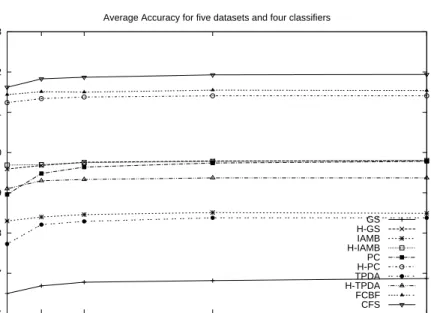
Figure 3 - 6 show the average percent accuracy, AUC and FNR of five datasets from all four classifiers. From average accuracy in figure 3, correlation-based feature selection (FCBF, CFS) provides the best average accuracy. Hybrid correlation and causal feature selection has better accuracy than original causal feature selection. Hybrid method using PC algorithm (H-PC) has slightly lower average accuracy than correlation-based feature selection but has the ability to deal with high dimensional features. From figure 4, PC, CFS, TPDA and FCBF algorithm provide the best and
Table 3 Number of selected features from each algorithm.
Dataset Original Correlation-Based Causal-Based Hybrid algorithm
Feature FCBF CFS PC TPDA GS IAMB H-PC H-TPDA H-GS H-IAMB
LUCAS 11 3 3 9 10 9 11 2 3 2 2
LUCAP 143 7 36 121 121 16 14 21 22 17 13
REGED 999 18 18 N/A N/A 2 2 18 N/A 2 2
CINA 132 10 15 132 N/A 4 4 5 7 10 9
SIDO 4932 23 25 N/A N/A 17 17 2 3 1 2
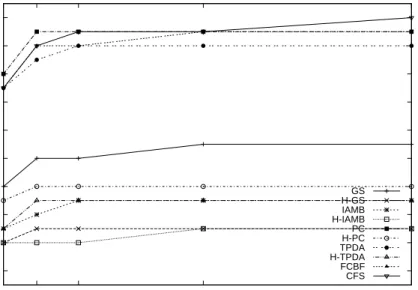
comparable AUC. Proposed hybrid algorithm has lower AUC than both correlation and original causal-based algorithms. In figure 5, H-PC has the lowest FNR. In all experiments, hybrid algorithm provides lower FNR than original causal algorithm but still higher than correlation-based algorithm.
86 87 88 89 90 91 92 93 1 5 10 25 50 Percent Accuracy Number of Classifiers
Average Accuracy for five datasets and four classifiers
GS H-GS IAMB H-IAMB PC H-PC TPDA H-TPDA FCBF CFS
Fig. 3 Average Percent Accuracy of five datasets and four classifiers
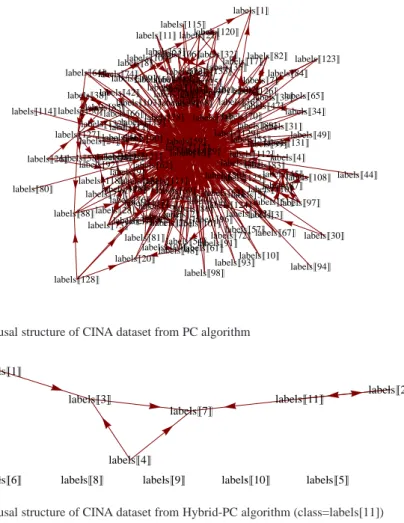
Figure 6 and 7 present examples of the causal structure for CINA dataset using PC and Hybrid-PC algorithm, respectively. The high complexity of original CINA dataset using PC algorithm can be seen in figure 6 while after remove redundant and irrelevant features of CINA dataset using hybrid PC algorithm as shown in figure 7, the complexity of system is decreased, easier to understand and higher accuracy (figure 4) compare to using original PC algorithm.
0.76 0.78 0.8 0.82 0.84 0.86 0.88 0.9 0.92 0.94 1 5 10 25 50 AUC Number of Classifiers
Average AUC for five datasets and four classifiers
GS H-GS IAMB H-IAMB PC H-PC TPDA H-TPDA FCBF CFS
Fig. 4 Average AUC of five datasets and four classifiers
0.1 0.12 0.14 0.16 0.18 0.2 0.22 0.24 0.26 0.28 0.3 1 5 10 25 50
False Negative Rate
Number of Classifiers
Average False Negative Rate for five datasets and four classifiers
GS H-GS IAMB H-IAMB PC H-PC TPDA H-TPDA FCBF CFS
labelsP1T labelsP2T labelsP3T labelsP4T labelsP5T labelsP6T labelsP7T labelsP8T labelsP9T labelsP10T labelsP11T labelsP12T labelsP13T labelsP14T labelsP15T labelsP16T labelsP17T labelsP18T labelsP19T labelsP20T labelsP21T labelsP22T labelsP23T labelsP24T labelsP25T labelsP26T labelsP27T labelsP28T labelsP29T labelsP30T labelsP31T labelsP32T labelsP33T labelsP34T labelsP35T labelsP36T labelsP37T labelsP38T labelsP39T labelsP40T labelsP41T labelsP42T labelsP43T labelsP44T labelsP45T labelsP46T labelsP47T labelsP48T labelsP49T labelsP50T labelsP51T labelsP52T labelsP53T labelsP54T labelsP55T labelsP56T labelsP57T labelsP58T labelsP59T labelsP60T labelsP61T labelsP62T labelsP63T labelsP64T labelsP65T labelsP66T labelsP67T labelsP68T labelsP69T labelsP70T labelsP71T labelsP72T labelsP73T labelsP74T labelsP75T labelsP76T labelsP77T labelsP78T labelsP79T labelsP80T labelsP81T labelsP82T labelsP83T labelsP84T labelsP85T labelsP86T labelsP87T labelsP88T labelsP89T labelsP90T labelsP91T labelsP92T labelsP93T labelsP94T labelsP95T labelsP96T labelsP97T labelsP98T labelsP99T labelsP100T labelsP101T labelsP102T labelsP103T labelsP104T labelsP105T labelsP106T labelsP107T labelsP108T labelsP109T labelsP110T labelsP111T labelsP112T labelsP113T labelsP114T labelsP115T labelsP116T labelsP117T labelsP118T labelsP119T labelsP120T labelsP121T labelsP122T labelsP123T labelsP124T labelsP125T labelsP126T labelsP127T labelsP128T labelsP129T labelsP130T labelsP131T labelsP132T labelsP133T
Fig. 6 Causal structure of CINA dataset from PC algorithm
labelsP1T labelsP2T labelsP3T labelsP4T labelsP5T labelsP6T labelsP7T
labelsP8T labelsP9T labelsP10T
labelsP11T
Fig. 7 Causal structure of CINA dataset from Hybrid-PC algorithm (class=labels[11])
Ensemble classifiers using Bagging slightly improves accuracy and AUC for most algorithms. Bagging also reduces FNR for CFS, PC and TPDA algorithm but provides stable FNR for the rest. After increasing number of classifiers to 5-10, the graphs of average accuracy, AUC and FNR all reach saturation point.
6 Discussion
In high dimensional features spaces, Bagging algorithm is not appropriate and im-practical for Bayesian Networks and its complexity may overestimate extra edges and their distribution might not satisfy Markov Blanket condition and faithfulness
condition [13], [14]. Therefore, this chapter proposed to solve this problem by re-ducing dimensionality before bagging while preserving efficiency and accuracy.
For small and medium number of features, the selected features after removing redundancy might be very small (may be only 2-3 features in some datasets and algorithms), however, the result is still comparable to the result before removing redundant features.
PC algorithm has tendency to select all features (all connected such as in CINA dataset) that may be impractical due to computational expense. Therefore, removing redundant features prior to causal discovery would benefit PC algorithm.
In some cases such as REGED dataset as shown in table 4, TPDA algorithm can have very complex causal relations between features that might be impractical to calculate even for medium number of features.
From the experiment results, Bagging can improve system accuracy and AUC but cannot improve FNR.
7 Conclusion
In this chapter, hybrid correlation and causal feature selection for ensemble classi-fiers is presented to deal with high dimensional features. According to the results, the proposed hybrid algorithm provides slightly lower accuracy, AUC and higher FNR than correlation-based. However, compared to causal-based feature selection, the proposed hybrid algorithm has lower FNR, higher average accuracy and AUC than original causal-based feature selection. Moreover, the proposed hybrid algo-rithm can enable PC and TPDA algoalgo-rithms to deal with high dimensional features while maintaining high accuracy, AUC and low FNR. Also the underlying causal structure is more understandable and has less complexity. Ensemble classifiers using Bagging provide slightly better results than single classifier for most algorithms. Fu-ture work will improve accuracy of search direction in strucFu-ture learning for causal feature selection algorithm.
References
1. Aliferis, C.F., Tsamardinos, I., Statnikov, A.: HITON, A Novel Markov Blanket Algorithm for Optimal Variable Selection. AMIA 2003 Annual Symposium Proceedings, pp 21–25 (2003) 2. Almuallim, H., Dietterich, T.G.: Learning with many irrelevant features. In: Proceedings of the
Ninth National Conference on Artificial Intelligence, pages 547–552 AAAI Press (1991) 3. Bauer, E., Kohavi, R.: An empirical comparison of voting classification algorithms: Bagging,
boosting, and variants. Machine Learning, 36(1-2):105-139 (1999)
4. Breiman, L.: Bagging predictors. Machine Learning, 24(2), 123–140 (1996)
5. Brown, L.E., Tsamardinos, I.: Markov Blanket-Based Variable Selection. Technical Report DSL TR-08-01 (2008)
6. Cheng, J., Bell, D.A., Liu, W.: Learning Belief Networks from Data : An Information theory Based Approach. In: Proceedings of the Sixth ACM International Conference on Information and Knowledge Management. pp 325–331 (1997)
7. Friedman, N., Nachman, I., Peer, D.: Learning of Bayesian Network Structure from Massive Datasets: The “Sparse Candidate” Algorithm. Proceedings of the 15th Conference on Uncer-tainty in Artificial Intelligence (UAI) Morgan Kaufmann, Stockholme, Sweden, pp 206–215 (1999)
8. Hall, M.A.: Correlation-based feature selection for discrete and numeric class machine learning. In: Proceeding of the 17th International Conference on Machine Learning, pp. 359–366. Morgan Kaufmann, San Francisco (2000)
9. Duangsoithong, R., Windeatt, T.: Relevance and Redundancy Analysis for Ensemble Classi-fiers. In: Perner,P. (ed.) Machine Learning and Data Mining in Pattern Recognition, vol. 5362, pp. 206–220, Springer, Heidelberg (2009)
10. Guyon, I., Aliferis, C., Elisseeff, A.: Causal Feature Selection. In: Computational Methods of Feature Selection, Liu, H. and Motoda, H. editors. Chapman and Hall (2007)
11. Guyon, I.: Causality Workbench (2008) http://www.causality.inf.ethz.ch/home.php
12. Kudo, M., Sklansky, J.: Comparison of algorithms that select features for pattern classifiers. Pattern Recognition, vol. 33, pp 25–41 (2000)
13. Liu, F., Tian, F., Zhu, Q.: Bayesian Network Structure Ensemble Learning. vol.4632/2007, pp 454–465. Springer Heidelberg (2007)
14. Liu, F., Tian, F., Zhu, Q.: Ensembling Bayesian Network Structure Learning on Limited Data. In: Proceeding of the 16th ACM conference on Conference on information and knowledge man-agement, pp 927–930. Association for Computing Machinery, New York, USA (2007) 15. Liu, H., Yu, L.: Toward integrating feature selection algorithms for classification and
cluster-ing. IEEE Transactions on Knowledge and Data Engineering 17(4), 491–502 (2005)
16. Margaritis, D., Thrun, S.: Bayesian network induction via local neighborhoods. In: Solla, S.A., Leen, T.K., Mller, K.-R. (eds.), Proceedings of the 1999 Conference 2000, vol. 12. MIT Press. pp 505-511 (2000)
17. Pudil, P., Novovicova, J., Kittler, J.: Floating Search Methods in Feature Selection. Pattern Recognition Letters, 15, 1119–1125 (1994)
18. Saeys, Y., Inza, I., Larranaga, P.: A review of feature selection techniques in bioinformatics. Bioinformatics 23(19), 2507–2517 (2007)
19. Spirtes, P., Glymour, C., Schinese, R.: Causation, Prediction, and search. Springer, New York (1993)
20. Tsamardinos, I., Aliferis, C.F., Statnikov, A.: Time and Sample Efficient Discovery of Markov Blankets and Direct Causal Relations. KDD2003 Washington DC, USA (2004)
21. Tsamardinos, I., Brown, L.E., Aliferis, C. F.: The max-min hill-climbing Bayesian network structure learning algorithm. Machine Learning, vol.65, pp 31–78 (2006)
22. Wang, M., Chen, Z., Cloutier, S.: A hybrid Bayesian network learning method for constructing gene networks. In: Computational Biology and Chemistry, vol. 31, pp 361–372 (2007) 23. Windeatt, T.: Accuracy/diversity and ensemble MLP classifier design. IEEE Transactions on
Neural Networks 17(5), 1194–1211 (2006)
24. Windeatt, T.: Ensemble MLP Classifier Design, vol. 137, pp.133–147. Springer, Heidelberg (2008)
25. Witten, I.H., Frank, E.: Data Mining: Practical Machine Learning Tools and Techniques. Mor-gan Kaufmann, San Francisco, 2 edition (2005)
26. Yu, L., Liu, H.: Efficient feature selection via analysis of relevance and redundancy. J. Mach. Learn. Res. 5, 1205–1224 (2004)
27. Zhang, H., Sun, G.: Feature Selection using Tabu search. Pattern Recognition, vol. 35, pp 701–711 (2002)