Fast (Re-)Configuration of Mixed On-demand and Spot
Instance Pools for High-throughput Computing
Alexandra Vintila
Dept. of Computer Science Vrije Universiteit Amsterdam, The Netherlands
[email protected]
Ana-Maria Oprescu
Institute of Informatics Universiteit van Amsterdam Amsterdam, The Netherlands
[email protected]
Thilo Kielmann
Dept. of Computer Science Vrije Universiteit Amsterdam, The Netherlands
[email protected]
ABSTRACT
Commercial cloud offerings let users allocate compute re-sources on demand, charging based on reserved time in-tervals. While this gives great flexibility to elastic high-throughput applications, users lack guidance for assembling instance pools from different cloud instance types, in order to meet given constraints, both with respect to completion time and the monetary budget for a computation. BaTS, our budget-constrained scheduler uses tiny statistical sam-ples of task executions in order to predict completion times (and associated costs) for given bags of tasks [13], for a small set of solutions that either favor fast execution or low com-putation budget. However, BaTS’ estimator can not handle variably-priced spot instances appropriately.
In this work, we present a new prediction module for BaTS that quickly computes accurate approximations to the Pareto set of mixed on-demand and spot instance pools, based on a genetic algorithm (GA). This new approach al-lows BaTS to react to changing spot instance prices at run-time by re-configuring the instance pool according to the user’s runtime and budget constraints. Simulator-based re-sults show that the GA can approximate the Pareto sets for machine configurations in about 30 seconds time, without noticeable loss of quality when compared to an offline com-putation of an exact solution that takes in the order of 40 to 60 minutes to compute.
1.
INTRODUCTION
In high-throughput computing, parameter sweep or bag-of-tasks applications are as dominant as computationally de-manding. An ideal match for these demands can be seen in commercial cloud offerings, like Amazon’s EC2 [5, 6], where computers can be allocated (“rented”) for given time inter-vals. The various commercial offerings differ not only in price, but also in the types of machines that can be allo-cated. While all machine types are described in terms of CPU clock frequency and memory size, it is not clear at all which machine type can execute a given user application
Permission to make digital or hard copies of all or part of this work for personal or classroom use is granted without fee provided that copies are not made or distributed for profit or commercial advantage and that copies bear this notice and the full citation on the first page. To copy otherwise, to republish, to post on servers or to redistribute to lists, requires prior specific permission and/or a fee.
Copyright 20XX ACM X-XXXXX-XX-X/XX/XX ...$15.00.
faster than others, let alone predicting which machine type can yield the best price-performance ratio. The problem of allocating the right number of machines, of the right type, for the right time frame, strongly depends on the application program, and is left to the user.
This problem is addressed by BaTS, our budget-constrained scheduler for bags of tasks [13].1 BaTS requires no a-priori information about task completion times. In a small, initial sampling phase, BaTS learns properties of the bag’s run-time distribution for each considered cloud offering. BaTS provides the user with a list of makespan/cost options (with different combinations of machines) to choose from, ranging from the cheapest to the fastest offer.
Our current implementation, however, provides only a small and fixed list of possible makespan/cost options, namely the cheapest option, the cheapest plus 10 % and plus 20 % of budget, as well as the fastest option, and the fastest mi-nus 10 % and mimi-nus 20 % of budget. This set of options might contain duplicates or obviously unattractive sched-ules. Instead, the Pareto set of options should be presented to the user as those are dominating all other possible ma-chine configurations. Another drawback of BaTS’s current makespan/cost prediction module is that it uses a bounded-knapsack solver tailored for typical price ranges of on-demand instance types, which renders it unfit to deal with the com-bined price range of spot and on-demand instances.
In this paper, we overcome these deficiencies of our previ-ous BaTS implementation. We have implemented a genetic algorithm that computes approximations to the Pareto set of makespan/cost options (based on their underlying instance pool configurations). This genetic algorithm allows BaTS to quickly (within seconds) compute a set of Pareto-optimal configurations, and hence is able to quickly react to changing spot instance prices.
We have evaluated the quality of the Pareto sets identified by our genetic algorithm using our BaTS simulator [14] that we have extended by price history logs from Amazon’s spot market. We compare our solutions to offline computations of the exact Pareto sets, both in terms of quality and of computational effort needed. Our results show that the GA can approximate the Pareto sets for machine configurations in about 30 seconds time, without noticeable loss of qual-ity when compared to an offline computation of an exact solution that takes in the order of 40 minutes to compute.
This paper is structured as follows. Sec. 2 describes the BaTS scheduler and discusses related work. Sec. 3 presents
1BaTS is implementing the Task Farming Service of the
our new genetic algorithm for approximating Pareto sets. We evaluate its performance in Sec. 4. Conclusions are drawn in Sec. 5.
2.
BACKGROUND AND RELATED WORK
Before we present our new genetic algorithm for predicting makespan/cost combinations of instance pools, we briefly summarize the basics of our BaTS scheduler, consider Pareto optimality, and discuss related work.
2.1
The BaTS Scheduler
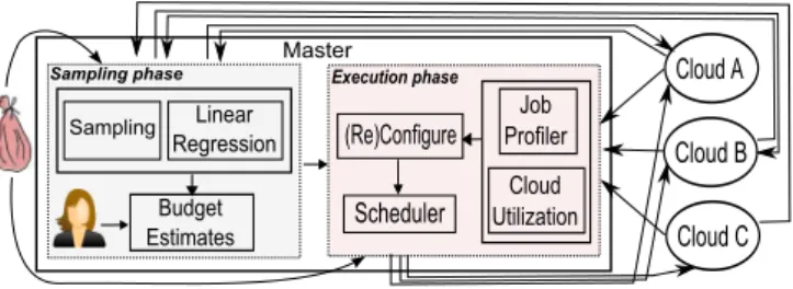
BaTS is scheduling large bags of tasks onto multiple cloud platforms. The individual tasks are scheduled in a self-scheduling manner onto the allocated machines. An initial sampling phase computes a list of budget estimates provid-ing the user with flexible control over budget and makespan. The execution phase allocates a number of machines from different clouds, and adapts the allocation regularly by ac-quiring and/or releasing machines in order to minimize the overall makespan while respecting the given budget limita-tion.
Figure 1: BaTS sampling phase (left) and execution phase (right).
Our task model needs no prior knowledge about the task execution times; it only needs the total number of tasks. About the machines, we assume that they belong to cer-tain categories (e.g. EC2’s “Standard Large”) and that all machines within a category are homogeneous. The only in-formation BaTS uses about the machines is their (hourly) price.
In this work, we use fixed hourly prices for on-demand instances and add information about the fluctuating prices for spot instances, based on spot price history provided by Amazon. As our focus is on computing the configurations of instance pools, we leave bidding strategies for the spot instances to future work; instead we assume that BaTS will place sufficiently high bids that avoid instance preemption. Bidding strategies for spot instances merely trade chances of not being preempted against acceptable price increases. With the work presented here, we can instead quickly drop too-expensive spot instance types and request more cost-efficient ones instead.
Figure 1 sketches BaTS’ overall system architecture. BaTS itself runs on a master machine, where the bag of tasks is available. Figure 1(left) sketches the sampling phase, where BaTS learns the bag’s stochastic properties and uses linear regression to translate task completion times across clouds [13]. In the sampling phase, all available machine types are tested; it is sufficient to sample a machine type only once, either under on-demand or under spot allocation: the machine type is the same, independent of the billing scheme.
BaTS generates a list of budget estimates accordingly, re-flecting execution speed and profitability (price/performance ratio). The user is then asked to select one of the budgets (e.g., faster or cheaper) corresponding to a desired sched-ule. The user’s choice then determines the machines al-located by BaTS for the execution phase, shown in Fig-ure 1(right). Here, BaTS allocates machines from various clouds and lets the scheduler dispatch the tasks to the cloud machines. Feedback, both about task completion times and cloud utilization, is used to reconfigure the clouds periodi-cally, as needed.
In this work, we improve on the existing budget/makespan estimation module, that is based on a bounded-knapsack solver, which provides only solutions of limited usefulness while being computationally demanding, also by the amount of memory needed to investigate the problem space. As our goal is to exploit combinations of on-demand and spot market instances, we need a new estimation module can can quickly handle the large problem space created by the spot instance prices that are both fluctuating and are an order of magnitude lower than the corresponding on-demand prices of the respective instance types.
It is worth mentioning that our very general task model does not allow any hard budget guarantees for the execution of the entire bag. Since BaTS has no a-priori information about the individual execution time of each task, we cannot guarantee that a certain budget will be definitely sufficient. The case might always occur that one or more outlier tasks, with exceptionally high completion time, might be scheduled only towards the end of the overall execution. In [14], we presented an optimization for the tail phase execution that reduces the severeness of this problem.
2.2
Pareto dominance, Pareto optimality and
Pareto fronts
Formal definitions [7] of Pareto dominance, optimality and fronts are legion. Intuitively, a problem that requires op-timizing multiple objectives has several aspects: first, the input variables representing the available types of resources and their respective ranges. Secondly, the objectives, which are (possibly conflicting) functions of these variables. Thirdly, the feasibility space, that is the range of possible values for each objective function, given the ranges of the input vari-ables.
The optimization takes place in the feasibility space, find-ing the best possible combinations of objective values, which will be mapped back to the corresponding combination of values of input variables (called a solution). The tough problem is deciding which are the best possible combina-tions, that is the best points in the feasibility space. Here, Pareto introduced the concept of dominance, which simply states that if a given solutionS1 outperforms another
solu-tionS2for at least one objective function, while it performs
equally well for the remaining objective functions, thenS1
dominates S2 (is strictly better). Based on this, aPareto optimal solution is a non-dominated one (no other solution is strictly better). The set of all non-dominated solutions corresponds to a set of points in the feasibility space, called aPareto front orPareto set.
The goal of our work is to compute the set of Pareto-optimal instance pools for a given bag of tasks, within the limitations on the numbers of available instances per type given by the cloud provider. Because computing the precise
Pareto set is computationally challenging, we present a ge-netic algorithm that can quickly compute an approximation to the precise Pareto set.
2.3
Related Work
High-throughput computing systems are legion, dating back to Condor [10]. Our own previous work on BaTS [13] and the work in [11] focus on executing bags of tasks in a high-throughput manner on cloud platforms, while keeping both execution makespan and monetary cost under control. Here, we extend BaTS by a means to quickly estimate the Pareto front of instance configurations, extending the appli-cability of BaTS to spot market instances and combinations of on-demand and spot instances.
The ExPERT framework [2] constructs the Pareto-frontier of scheduling strategies from which it selects the one that best fulfills a user-provided utility function. Unlike Ex-PERT, we focus on the makespan of the execution as a whole, and we compute the Pareto front of machine (cloud instance) combinations on which BaTS executes the tasks of a bag in a self-scheduling manner.
There are many genetic algorithms investigating resource selection and job scheduling. Our work has been inspired by [15], where the authors build a genetic algorithm to ap-proximate the Pareto frontier of schedules for jobs and data transfers in grid environments. Their method does not scale well with the number of jobs to be executed, as their gene encoding has one entry per job in each chromosome. In-stead, we only encode the numbers of instances per instance type within our chromosomes, which is independent of the actual number of tasks, and hence scales to the execution of large bags.
3.
GENETIC ALGORITHM
We start from a typical genetic algorithm structure (Al-gorithm 1): iterate over a number of generations (popu-lations) until the algorithm converges according to a ter-mination condition. In each iteration, new individuals are randomly generated or created through recombination and mutation. The new individuals together with an elite of the current population form an intermediate population. A second selection step chooses among the extended (interme-diate) population those individuals that will become part of the new population, that is the generation of the next it-eration. During the selection process, a fitness function is used to rank individuals. The result of the algorithm is the estimated Pareto front.
3.1
Chromosome and gene encodings
In genetic algorithms, a population contains a number of chromosomes (individuals), and each chromosome consists of an (equal) number of genes. Their mapping to the real-world problem widely varies from domain to domain.
In our approach, a chromosome represents a configura-tion of machines from different types. A gene encodes the number of machines of a certain type (including zero) and is represented as an integer. Thus, a chromosome is rep-resented as an integer array. Table 1 shows an example of a chromosome encoding for a valid machine configuration given a pool of the following Amazon EC2 instance types: t1.micro, m1.small, m1.medium in both pricing policies: on-demand [5] and spot [6]. Therefore, we get a total of 6 genes. We have chosen this type of representation because it is
Algorithm 1Genetic Algorithm to Estimate Pareto Fronts
Input: machine types
Output: estimated Pareto front 1: population[POPULATION_SIZE]
2: forfixed number of iterationsdo
3: whilepopulation array is not fulldo
4: addrandom valid chromosome to population
5: end while
6: for allchrm C in populationdo
7: C.fitness←computeFitness(C)
8: end for
9: population←selectNewPopulation(population)
10: end for
11: buildParetoFront(population)
12: if Pareto front size<threshold then
13: go once to line 2 14: end if
15: returnthe biggest Pareto front found
Algorithm 2computeFitness
Input: chromosome C
Output: fitness value
1: maxCost←maximum cost found in population 2: minCost←minimum cost found in population 3: diffCost←maxCost - minCost
4: maxMsp←max makespan in population 5: minMsp←min makespan in population 6: diffMsp←maxMsp - minMsp
7: // clCost - closeness to min cost (%) 8: // clMsp - closeness to min mspan (%) 9: clCost←(maxCost−C.cost + 1)/diffCost 10: clMsp←(maxMsp−C.msp + 1)/diffMsp 11: returnMax(clCost, clMsp)·clCost·clMsp
more suitable for our problem than the traditional binary representation of a chromosome. By having integers as genes it is easier to compute the makespan and cost of a schedule, as well as to check the validity of the chromosome with re-spect to certain constraints. Each machine type has a limit on the number of machines the user can acquire. Another constraint is the limit on the overall number of machines.
3.2
Fitness function
In order to estimate the Pareto front, we need to find those individuals in the population that are closest to the Pareto front, that is the individuals which minimize both our objective functions: cost and makespan. To estimate their closeness to the Pareto front (given that it is a-priori unknown), we use a fitness function, where intuitively the larger its value, the better the individual. The fitness value of a chromosome is (re-)computed for each iteration.
Our objective functions incur different ranges of values: we deal with time versus money. In order to handle this, we split the search space, by predefined numbers for both the cost and the makespan ranges. This results in a grid struc-ture layout of the search space, each chromosome belonging to a cell. The numbers used for splitting determine the accu-racy of the fitness function in discriminating between chro-mosomes and help in handling overfitting and underfitting. Our fitness function considers closeness indicators that are normalized with respect to the value ranges. That is, we use
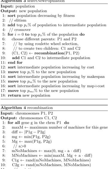
Algorithm 3selectNewPopulation
Input: population
Output: new population
1: sortpopulation decreasing by fitness 2: // elitism
3: addtoppe% of population to intermediate population
4: // crossover
5: fori= 0totoppx% of the populationdo
6: choose different parents: P1 and P2 7: // by using roulette wheel selection, 8: // to create two children: C1 and C2 9: (C1, C2)←recombination(P1, P2) 10: addC1 and C2 to intermediate population 11: end for
12: sortintermediate population increasing by cost 13: movetoppc% to the new population
14: sortintermediate population increasing by makespan 15: movetoppm% to the new population
16: sortintermediate population increasing by msp+cost 17: movetoppmc% to the new population
18: returnnew population
Algorithm 4recombination
Input: chromosomes P1, P2
Output: chromosomes C1, C2
1: for allgene g in the chrm P1 do
2: maxM←maximum number of machines for this gene 3: diff← |P1g−P2g|
4: mg←min(P1g, P2g)
5: Mg←max(P1g, P2g)
6: // a>0
7: mNoMachines←max(0, mg - a·diff) 8: MNoMachines←min(maxM, Mg + a·diff) 9: C1g←rand(mNoMachines, MNoMachines)
10: C2g←rand(mNoMachines, MNoMachines)
11: // mutation
12: flipa bit in C1g, C2g with probabilitypf
13: end for
14: returnC1, C2
the relative cell distance of the predicted makespan of a chro-mosome C to the largest predicted makespan found in the current population as amakespan indicator (the bigger the distance, the better the chromosome). We use the relative cell distance of the chromosome’s corresponding estimated cost (necessary budget) to the largest estimated cost in the current population as acost indicator.
We also reward the individuals that excel in either ob-jective function (cost or makespan) as shown in line 11 of Algorithm 2. The chromosomes which are farther situated from at least one objective’s maximum values will have a higher fitness value. The effect of giving extra weight to the superior objective value of a chromosome is that the current Pareto front is slowly pushed towards the small values of both objective ranges.
3.3
Population selection
The population selection must ensure a trade-off between the quality and the diversity of the next generation’s individ-uals. To that end, genetic algorithms use such mechanisms as elitist selection, crossover operations and mutations.
Algorithm 5 Algorithm for Building Pareto Fronts from
GA Population: buildParetoFront
Input: population Pop
Output: estimated Pareto front 1: sortPop increasing by makespan 2: i←1
3: add Pop[i] to the Pareto front
4: find smallest j>i such that the Pop[j].cost<Pop[i].cost 5: if no j is foundthen
6: return
7: else
8: i←j
9: continuefrom line 3
10: end if
gene1 gene2 gene3 gene4 gene5 gene6
micro small medium spot.micro spot.small spot.medium
39 28 15 50 65 20
Table 1: Example of a chromosome containing genes for six machine types.
Our population selection is done in two main steps. First, we build the intermediate population (lines 1–11 in Algo-rithm 3). Next, we select the best chromosomes by cost, makespan and their sum (lines 12–17 in Algorithm 3).
We initialize the intermediate population with the toppe
(%) fittest chromosomes of the current population, a tech-nique known aselitism in genetic algorithms.
Next, we extract a number of pairs equal to a percent-age px from the population. Each individual is selected
based on roulette wheel selection (fitness proportional se-lection [1]). From each pair we obtain two children using blend crossover (BLX-a Crossover [8]), as shown in Algo-rithm 4, lines 1–10. We choose this crossover technique as it proved to give the lowest number of invalid children chro-mosomes. For instance, when using the two point crossover operation, adapted to our chromosome type, more than half of the children were invalid. BLX-a is the best approach because it generates a controllable amount of values within the bounds of the parent genes, which already respect all the constraints. Therefore, the probability of building an invalid child may be easily adjusted.
We are also interested in children that lie just outside the parents gene range, but within the allowed number of ma-chines per type. Such children increase the diversity of the population and may be the key to a finding better perform-ing machine configurations.
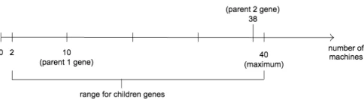
We ensure all created children are valid by properly ad-dressing all corner cases (e.g. equal parents genes). A nu-merical example of the BLX-a crossover is shown in Figure 2. Here, parent 1 contains 10 machines of a certain type M, while parent 2 has 38 machines of the same type. Assuming
a= 0.3 and according to line 8 in Algorithm 4, the pool of genes for their children will consist of all integers between 2 and 40, from which we choose randomly.
We apply the mutation operation on each new child gene with a certain probability, pf. The mutation consists of
flipping a random bit in the integer representing the gene (Algorithm 4 line 12).
Figure 2: A numerical example of BLX-a recombi-nation (with a=0.3) for a machine of type M.
population and returns the next generation. This step is an optimization of the classical genetic algorithm and has the purpose of selecting, based on their cost and budget objec-tives, the top machine configurations for the next population (ensuringquality). A small percentage (100-pc-pm-pmc) of
the chromosomes with the lowest fitness in the intermedi-ate population is always left behind, in order to make room for new randomly generated individuals (ensuringdiversity). As a consequence, we make sure that the algorithm explores the state space.
3.4
Pareto Front
From the population resulted after the genetic algorithm’s iterations, we build the Pareto front, using Algorithm 5. The number of schedules in the set is lower than the one of the schedules found in the real Pareto front. More about the size of the estimated Pareto Front compared to the real Pareto front in the Section 4.5.
We use a simple heuristic to control the size of the es-timated Pareto front (line 12 in Algorithm 1): if the size is below a certain (fixed) threshold, we re-execute the ge-netic algorithm with the same number of iterations. In any case, we take the Pareto front with the maximum number of elements. This situation has a very low probability of happening, decreasing as the size of the population grows.
4.
EVALUATION
Our algorithm approximates the Pareto front by construct-ing a set of (locally) Pareto-optimal solutions. Given the nature of a genetic algorithm, we cannot guarantee that we generate the entire feasible space of the optimization prob-lem, and therefore the Pareto optimal solutions obtained by our approach may be dominated by solutions outside the considered feasible subspace. Another consequence of using a feasible subspace is a (possibly) incomplete Pareto front. We addressed these limitations with a set of heuristics applied during the recombination, mutation and selection steps, next to a tailored termination condition. Therefore, we evaluate our genetic algorithm for Pareto set approxi-mation with respect to both its optimality and its size by comparison to the corresponding real Pareto set.
Next, we evaluate the runtime performance of the genetic algorithm compared to the exhaustive search used to com-pute the real Pareto set offline. We analyze these aspects on several workloads that have been found representative for real-world bag-of-tasks applications [14].
4.1
Simulated mixes of cloud instances
We simulate two different types of instance mixes, inspired by behavior of Amazon EC2, which are relevant for real-world scenarios:
(a) An equal limit on all instance types, where the user has access to a pool of in total 100 cloud instances with an upper bound of 20 for each instance type, referred to as20-100;
(b) Different limits for on-demand instance types versus spot-instances, where the user has access to a pool of maximum 100 cloud instances with an upper bound of 40 for each on-demand instance type and 60 for each spot instance type, referred to as40-60-100.
Each on-demand instance type has an associated price and (simulated) execution speed. For each on-demand instance type we simulate a corresponding spot instance type, with the same characteristics, but a different (bidding) price. In total, we use six instance types:
• t1.micro - executes tasks according to their generated runtime and costs $0.020 per hour;
• m1.small- executes tasks twice as fast as ”t1.micro” and costs $0.065 per hour;
• m1.medium- executes tasks three times as fast as ”t1.small” and costs $0.130 per hour;
• spot t1.micro- same speed as ”t1.micro” and costs $0.003 per hour;
• spot m1.small - same speed as ”m1.small” and costs
$0.007 per hour;
• spot m1.medium - same speed as ”m1.medium” and
costs $0.013 per hour;
4.2
Workloads
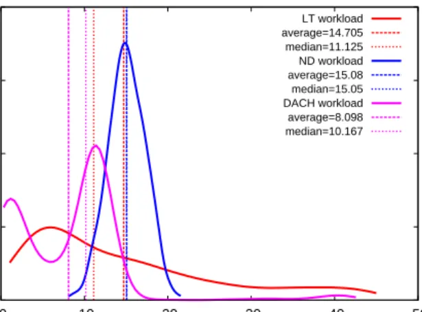
We evaluate our genetic algorithm on three different kinds of workloads, modeled after real bags of tasks, using a nor-mal distribution, a Levy-truncated distribution, and a mix-ture of distributions. Each workload contains 1000 tasks, with runtimes generated according to the respective distri-bution type.
Normal distribution has been identified as relevant for bag-of-tasks workloads by research conducted in [9]. Ac-cordingly, we have generated a workload following the nor-mal distributionN(15, σ2), σ=√5 (in minutes, see Fig. 3),
abbreviated asNDB(”normal distribution bag”).
Research based on large traces [12] shows that some bags of tasks have a skewed distribution, bounded by some max-imum value. To model such bags, we generate workloads according to a truncated Levy distribution with a scaling factor (τ) of 12 minutes and a maximum value (b) of 45 minutes, as shown in Fig. 3, abbreviated as LTB (”Levy-truncated distribution bag”).
Another real application was provided by The First Inter-national Data Analysis Challenge for Finding Supernovae (DACH) [3]. The task runtimes depicted in Fig. 3 were obtained by running the entire workload on a reference ma-chine. We model this workload as a mixture of distributions generating workloads of which task runtimes exhibit a root-mean square deviation from the real workload of less than 5%. We refer to the corresponding workload as a multi-modaldistribution bag, abbreviated asMDB(”multi-modal distribution bag”).
0 0.05 0.1 0.15 0.2 0 10 20 30 40 50 fraction minutes LT workload average=14.705 median=11.125 ND workload average=15.08 median=15.05 DACH workload average=8.098 median=10.167
Figure 3: Distribution types used for workloads gen-eration: normal distribution (NDB) with an expec-tation of 15 min., Levy-truncated (LTB) with an up-per bound of 45 min. and a real-world multi-modal distribution (DACH).
4.3
Generation of Real Pareto Front
To evaluate the estimated Pareto fronts resulted from our genetic algorithm, we have implemented an exhaustive-search algorithm to generate the real (precise) Pareto front. This algorithm explores the state (feasibility) space using an optimized backtracking approach.
We start building the Pareto front with the first two gen-erated schedules and progressively extend and improve the set. We reduce the state space by pruning the tree which has as a root an invalid machine configuration. Newly gen-erated machine configurations are added to the Pareto front if they are better than any of those already in the Pareto set. In this way, we avoid keeping in memory all the state space and build the Pareto front by iterating it.
4.4
Genetic Algorithm parameters
We use two different population sizes (POPULATION_SIZE): 1000 (1k) and 2000 (2k). The percentage of population se-lected by elitism (pe) is set to 20%. When performing the
crossover operation, we extract a number of pairs equal to a percentage,px set to 40%, from the population. The
per-centages of the intermediate population selected by cost (pc)
or by makespan (pm) are set to 20%. The percentage of the
intermediate population selected by a function of costand makespan (pmc) is set to 50%. For each gene, the probability
of mutation,pf, is 1/15000.
4.5
Experimental Results
First, we evaluate the quality of the estimated Pareto set (PS) from an optimality perspective, that is how close are our Pareto optimal solutions to the real ones. We perform two sets of experiments, one for each mix of cloud resources. We estimate the Pareto set for an instance of each workload type and we also compute the respective real Pareto set. Moreover, we evaluate the impact of the workload type on the accuracy of the estimated Pareto front. To that end, we executed our genetic algorithm with two different population sizes for the same instance of each workload type: 1000(1k)
and 2000(2k).
All the results are presented in a log-log scale in Fig-ures 4 (NDB), 5 (MDB) and 6 (LTB). The figures show our algorithm follows very closely the real Pareto front in every scenario. The main advantage of using a larger popu-lation is that our Pareto optimal points become sufficiently scattered across the real Pareto front, providing a proper range of relevant choices for the user.
0.1 1 10 100 0.1 1 10 100 1000 cost(dollars) time(hours) NDB 20-100 Real PS NDB 1k 20-100 Estimated PS NDB 2k 20-100 Estimated PS NDB 40-60-100 Real PS NDB 1k 40-60-100 Estimated PS NDB 2k 40-60-100 Estimated PS
Figure 4: NDB bag, real Pareto set (PS) versus es-timated Pareto set for pool mixes of type 20-100 and 40-60-100 , when using two different population sizes: 1000 (1k) and 2000 (2k). 0.1 1 10 100 0.1 1 10 100 1000 cost(dollars) time(hours) MDB 20-100 Real PS MDB 1k 20-100 Estimated PS MDB 2k 20-100 Estimated PS MDB 40-60-100 Real PS MDB 1k 40-60-100 Estimated PS MDB 2k 40-60-100 Estimated PS
Figure 5: MDB bag, real Pareto set (PS) versus estimated Pareto set for pool mixes of type 20-100 and 40-60-100 , when using two different population sizes: 1000 (1k) and 2000 (2k).
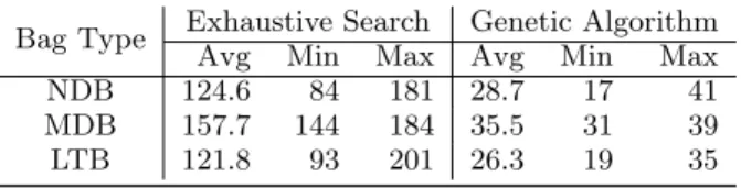
Next, we evaluate the quality of the estimated PS with respect to the length of the real Pareto front, obtained via an exhaustive (offline) approach. In Table 2 we summarize the results obtained by running each algorithm on ten differ-ent bag instances of each workload type in scenario20-100. The genetic algorithm used a population of 2000 (2k). We repeated the experiment for scenario40-60-100 and sum-marized the results in Table 3. Though the real Pareto front
0.1 1 10 100 0.1 1 10 100 1000 cost(dollars) time(hours) LTB 20-100 Real PS LTB 1k 20-100 Estimated PS LTB 2k 20-100 Estimated PS LTB 40-60-100 Real PS LTB 1k 40-60-100 Estimated PS LTB 2k 40-60-100 Estimated PS
Figure 6: LTB bag, real Pareto set (PS) versus es-timated Pareto set for pool mixes of type 20-100 and 40-60-100 , when using two different population sizes: 1000 (1k) and 2000 (2k).
is richer in quantity, we have already shown in Figures 4, 5 and 6 that our estimated Pareto front is similar in quality, providing a sufficient number of Pareto optimal solutions.
Table 2: Size of real and estimated Pareto sets on a mix of type 20-100, population size 2k
Bag Type Exhaustive Search Genetic Algorithm
Avg Min Max Avg Min Max
NDB 124.6 84 181 28.7 17 41
MDB 157.7 144 184 35.5 31 39
LTB 121.8 93 201 26.3 19 35
Table 3: Size of real and estimated Pareto sets on a mix of type 40-60-100, population size 2k
Bag Type Exhaustive Search Genetic Algorithm
Avg Min Max Avg Min Max
NDB 188.0 155 204 42.7 38 50
MDB 247.9 196 278 31.5 18 44
LTB 193.3 162 214 39.5 18 54
We use the same set of experiments to evaluate the run-time performance of our algorithm against the exhaustive (offline) approach. All experiments were performed on DAS4 [4] standard compute nodes (dual-quad-core 2.4 GHz CPU con-figuration and 24GB memory). The corresponding results are collected in Tables 4 and 5. As the problem size in-creases, our results show that the genetic algorithm categor-ically outperforms the exhaustive-search approach, reducing the time-to-solution from 40–60 minutes to about 30 sec-onds, which enables online reconfiguration of instance pools, for example in case of spot price changes.
5.
CONCLUSIONS
In previous work, we have demonstrated the efficacy of our BaTS scheduler for large bags of tasks on multiple cloud en-vironments [13, 14]. Without any a-priori knowledge of task
Table 4: Runtimes (sec) for computing real and es-timated Pareto sets on a mix of type 20-100, popu-lation size 2k
Bag Type Exhaustive Search Genetic Algorithm
Avg Min Max Avg Min Max
NDB 43.5 10 100 30.5 30 31
MDB 72.2 48 84 30.6 30 31
LTB 27.2 12 76 30.6 30 31
Table 5: Runtimes (sec) for computing real and esti-mated Pareto sets on a mix of type 40-60-100, pop-ulation size 2k
Bag Type Exhaustive Search Genetic Algorithm
Avg Min Max Avg Min Max
NDB 2748.0 1579 4207 31.1 31 32
MDB 3655.0 1937 5798 31.0 30 32
LTB 2500.3 1656 3826 31.1 31 32
runtimes, BaTS uses a tiny sample of tasks for estimating the price-performance ratios of the available types of cloud instances, for the given bag. Based on these ratios, BaTS computes a set of estimated makespan-cost alternatives for executing the bag, based on different instance pools that are composed of the available instance types. The user can then select one of these alternatives, expressing his or her pref-erence for either cost efficiency or execution speed. During the bulk execution of the bag, BaTS then monitors the exe-cution and adjusts, if necessary, the selected instance pool. This approach works pretty well, even though there are no hard guarantees (only stochastic properties) that the execu-tion schedule will stick to the estimated limits [14].
In this work, we overcome one weakness of BaTS, that is the quality of the presented makespan-cost alternatives. We replace the original, static set of alternatives by an approx-imation to the set of Pareto-optimal solutions, yielding a (mostly) complete set of useful instance type combinations. As this computation is very demanding, both in terms of computation complexity and memory requirements, we have implemented a genetic algorithm that computes an approx-imation to the precise Pareto set.
Our experiments show that computing the precise Pareto set takes in the order of 40 to 60 minutes on a regular com-pute node, which is only useful for offline computations. Our GA, however, approximates the exact Pareto set in about 30 seconds, which allows for quick re-configuration of in-stance pools at runtime, for example when using spot market instances that face fluctuations of their hourly prices (and hence price-performance ratios).
We have evaluated the quality of our GA-based approach using the simulator introduced in [14]. Based on bags with three different task runtime distributions (normal, heavy tailed, and a multi-modal mixture of distributions), we have shown that our GA computes approximations that deviate only marginally from the precise Pareto sets, and does so within seconds, enabling its use for fast and efficient recon-figurations at runtime.
We are currently integrating our GA-based approach into the BaTS implementation that is part of the ConPaaS plat-form, enabling the use of spot market instances, next to providing a large choice of Pareto-optimal solutions.
Nec-essary for this integration is further research into bidding strategies for spot instances that provide a trade-off between cost-efficiency and availability probabilities of the instances. Our new and fast GA-based estimator will enable such com-putations at runtime.
Acknowledgments
The research leading to these results has received funding from the European Union Seventh Framework Programme under grant agreement FP7-ICT-257438 (Contrail).
6.
REFERENCES
[1] Thomas B¨ack.Evolutionary algorithms in theory and practice: evolution strategies, evolutionary
programming, genetic algorithms. Oxford University Press, Oxford, UK, 1996.
[2] O. Agmon Ben-Yehuda, A. Schuster, A. Sharov, M. Silberstein, and A. Iosup. Expert: Pareto-efficient task replication on grids and a cloud. InIPDPS’12, 2012.
[3] The First International Data Analysis Challenge for Finding Supernovae.
http://www.cluster2008.org/challenge/. held in conjunction with IEEE Cluster/Grid 2008. [4] The Distributed ASCI Supercomputer (DAS4).
http://www.cs.vu.nl/das4/. [5] Amazon EC2 Instance Types.
http://aws.amazon.com/ec2/instance-types/. [6] Scientific Computing Using Spot Instances.
http://aws.amazon.com/ec2/spot-and-science/. [7] Matthias Ehrgott.Multicriteria Optimization (2. ed.).
Springer, 2005.
[8] T.D. Gwiazda.Genetic Algorithms Reference. Number v. 1 in Genetic Algorithms Reference. Tomasz
Gwiazda, 2006.
[9] Alexandru Iosup, Omer Ozan Sonmez, Shanny Anoep, and Dick H. J. Epema. The performance of
bags-of-tasks in large-scale distributed systems. In HPDC, 2008.
[10] Michael J. Litzkow, Miron Livny, and Matt W. Mutka. Condor-a hunter of idle workstations. In8th International Conference on Distributed Computing Systems, pages 104–111. IEEE, 1988.
[11] Ming Mao, Jie Li, and Marty Humphrey. Cloud auto-scaling with deadline and budget constraints. In Grid 2010, 2010.
[12] Tran Ngoc Minh, Lex Wolters, and Dick Epema. A realistic integrated model of parallel system workloads. InCCGRID’10, 2010.
[13] Ana-Maria Oprescu, Thilo Kielmann, and Haralambie Leahu. Budget estimation and control for bag-of-tasks scheduling in clouds.Parallel Processing Letters, 21(2):219–243, 2011.
[14] Ana-Maria Oprescu, Thilo Kielmann, and Haralambie Leahu. Stochastic Tail-Phase Optimization for Bag-of-Tasks Execution in Clouds. In5th IEEE/ACM International Conference on Utility and Cloud Computing (UCC 2012), Chicago, IL, USA, November 2012.
[15] Javid Taheri, Albert Y. Zomaya, and Samee U. Khan. Genetic algorithm in finding pareto frontier of
optimizing data transfer versus job execution in grids. Concurrency and Computation: Practice and