Single-Pass Online Learning: Performance, Voting
Schemes and Online Feature Selection
Vitor R. Carvalho
a aLanguage Technologies InstituteCarnegie Mellon University 5000 Forbes Avenue,Pittsburgh, PA
[email protected]
William W. Cohen
a,b bMachine Learning DepartmentCarnegie Mellon University 5000 Forbes Avenue,Pittsburgh, PA
[email protected]
ABSTRACT
To learn concepts over massive data streams, it is essential to design inference and learning methods that operate in real time with limited memory. Online learning methods such as perceptron or Winnow are naturally suited to stream pro-cessing; however, in practice multiple passes over the same training data are required to achieve accuracy comparable to state-of-the-art batch learners. In the current work we address the problem of training an on-line learner with a sin-gle pass over the data. We evaluate several existing meth-ods, and also propose a new modification of Margin Bal-anced Winnow, which has performance comparable to lin-ear SVM. We also explore the effect of averaging, a.k.a. vot-ing, on online learning. Finally, we describe how the new Modified Margin Balanced Winnow algorithm can be nat-urally adapted to perform feature selection. This scheme performs comparably to widely-used batch feature selection methods like information gain or Chi-square, with the ad-vantage of being able to select features on-the-fly. Taken together, these techniques allow single-pass online learning to be competitive with batch techniques, and still maintain the advantages of on-line learning.
Categories and Subject Descriptors
I.2.6 [Artificial Intelligence]: LearningGeneral Terms
Algorithms, Performance, Experimentation.
Keywords
Online Learning, Averaging, Voting, Winnow
1. INTRODUCTION
Compared to batch methods, online learning methods are often simpler to implement, faster, and require less mem-ory. For such reasons, these techniques are natural ones to consider for large-scale learning problems.
Permission to make digital or hard copies of all or part of this work for personal or classroom use is granted without fee provided that copies are not made or distributed for profit or commercial advantage and that copies bear this notice and the full citation on the first page. To copy otherwise, to republish, to post on servers or to redistribute to lists, requires prior specific permission and/or a fee.
KDD’06,August 20–23, 2006, Philadelphia, Pennsylvania, USA. Copyright 2006 ACM 1-59593-339-5/06/0008 ...$5.00.
Online learning algorithms have been traditionally trained using several passes through the training data [3, 11, 14]. In the current work we address the problem of single-pass online learning, i.e., online learning restricted to a single training pass over the available data. This setting is partic-ularly relevant when the system cannot afford several passes throughout the training set: for instance, when dealing with massive amounts of data, or when memory or processing re-sources are restricted, or when data is not stored but pre-sented in a stream.
In this paper, we experimentally compare the performance of different online learners to traditional batch learning in the single-pass setting, and we introduce a new online algo-rithm — MBW or Modified Balance Winnow — that out-performs all other single-pass online learners and achieves results comparable to Linear SVM in several NLP tasks.
Voting (a.k.a. averaging) an online classifier is a technique that, instead of using the best hypothesis learned so far, uses a weighted average of all hypotheses learned during a train-ing procedure. The averagtrain-ing procedure is expected to pro-duce more stable models, which leads to less overfitting [13]. Averaging techniques have been successfully used on the Perceptron algorithm [14], but never in other online learners such as Winnow, Passive-Aggressive[10] or ROMMA[16]. In the current work, we provide a detailed performance com-parison on how averaging affects the aforementioned online learners when restricted to a single learning pass only. Re-sults clearly indicate that voting improves performance of most mistake-driven learning algorithm, including learners to which it has not traditionally been applied.
We also propose an effective Online Feature Selection scheme based on the “extreme” weights stored by the MBW algorithm. Performance results indicate that this scheme shows surprisingly good accuracies in NLP problems, being competitive with Chi-Square or Information Gain, but having the advantage of being able to select the most meaningful features on-the-fly.
Below, section 2 presents different online learners, and introduces the MBW algorithm. Section 3 presents the av-eraging technique. Section 4 compares results and presents the first two contributions: the impressive results of MBW in NLP tasks, and the boost in performance obtained on non-NLP datasets by averaging classifiers. In section 5, we in-troduce a new MBW-based online feature selection scheme. Finally, section 6 presents our conclusions.
2. ONLINE LEARNING
format for mistake-driven online learning algorithms, illus-trated in Table 1. For each new examplext presented, the current model will make a predictionybt∈ {−1,1}and com-pare it to the true classyt∈ {−1,1}. The prediction will be based on the score functionf, on the examplextand on the current weight vectorwi. In the case of a prediction mis-take, the model will be updated. Different mistake-driven algorithms differ in terms of the score functionf and in the way the weight vectorswiare updated, as we shall detail in the next sections.
Table 1: Mistake-Driven Online Learner.
1. Initializei= 0, success counterci= 0, modelw0 2. Fort= 1,2, ..., T:
(a) Receive new examplext
(b) Predictybt=f(wi, xt), and receive true classyt (c) If prediction was mistaken:
i. Update modelwi→wi+1 ii. i=i+ 1
(d) Else: ci=ci+ 1
2.1 Winnow Variants
The Positive Winnow, Balanced Winnow and Modified Balanced Winnow algorithms are based on multiplicative updates. For all three, we assume the incoming examplext is a vector of positive weights, i.e.,xjt ≥0,∀tand∀j. This assumption is usually satisfied in NLP tasks, where thexjt values are typically the frequency of a term, presence of a feature, TFIDF value of a term, etc.
In preliminary experiments, we found that the Winnow variants performed better if we applied anaugmentationand a normalization preprocessing step, in both learning and testing phases. When learning, the algorithm receives a new examplext with m features, and it initially augments the example with an additional feature(the (m+ 1)thfeature), whose value is permanently set to 1. This additional feature is typically known as “bias” feature. After augmentation, the algorithm thennormalizesthe sum of the weights of the augmented example to 1, therefore restricting all feature weights to 0≤xjt ≤1.
In testing mode, the augmentation step is the same, but there is a small modification in thenormalization. Before the normalization of the incoming instance, the algorithm checks each feature in the instance to see if it is already present in the current model (wi). The features not present in the current model are then removed from the incoming instance before the normalization takes place.
2.1.1 Balanced Winnow
The Balanced Winnow algorithm is an extension of the Positive Winnow algorithm [17, 11]. Similar to Positive Winnow, it is based on three parameters: a promotion pa-rameterα >1, a demotion parameterβ, where 0< β <1, and a threshold parameterθth>0.
Lethxt, wiidenote the inner product of vectorsxtandwi. Here, the modelwtis a combination of two parts: a positive model ut and a negative model vt. The score function is f =sign(hxt, uii − hxt, vii −θth), and the update rule is:
For allj s.t. xj t >0, uji+1= ( uji·α ,ifyt>0 uji·β ,ifyt<0 and vij+1= ( vij·β ,ifyt>0 vij·α ,ifyt<0 The initial modelu0 andv0 are set to the positive values
θ+
0 and θ−0, respectively, in all dimensions. Despite their simplicity, Positive Winnow and Balanced Winnow are able to perform very well in different NLP tasks [3, 4, 11].
2.1.2 Modified Balanced Winnow
TheModified Balanced Winnow, henceforth MBW, is de-tailed in Table 2. Like Balanced Winnow, MBW has a pro-motion parameterα, a demotion parameterβand a thresh-old parameterθth. It also uses the same decision functionf as Balanced Winnow, as well as the the same initialization. However, there are two modifications.
The first modification is the “thick”-separator (or wide-margin) approach [11]. The prediction is considered mis-taken, not only whenyt is different fromybt, but also when the score function multiplied byytis smaller than the “mar-gin” M, where M ≥0. More specifically, the mistake con-dition is (yt·(hxt, uii − hxt, vii −θth))≤M.
The second modification is a small change in the update rules, such that each multiplicative correction will depend on the particular feature weight of the incoming example. The change is illustrated in Table 2.
Table 2: Modified Balanced Winnow (MBW).
1. Initializei= 0, counterci= 0, and modelsu0 andv0
2. Fort= 1,2, ..., T:
(a) Receive new examplext, and add “bias” feature.
(b) Normalizextto 1.
(c) Calculatescore=hxt, uii − hxt, vii −θth.
(d) Receive true classyt.
(e) If prediction was mistaken, i.e., (score·yt)≤M:
i. Update models. For all featurej s.t.xt>0 :
uji+1= ( uji·α·(1 +xjt) ,ifyt>0 uji·β·(1−xjt) ,ifyt<0 vji+1= ( vji·β·(1−xjt) ,ifyt>0 vji·α·(1 +x j t) ,ifyt<0 ii. i=i+ 1 (f) Else:ci=ci+ 1
2.2 Other Online Learners
Initially proposed in 1958 [21], thePerceptron learner al-gorithm uses a very simple and effective update rule. In spite of its simplicity, given a linearly separable training set, the Perceptron algorithm is guaranteed to find a solution that perfectly classifies the training set in a finite number of iterations.
Another learner, the Relaxed Online Maximum Margin Algorithm, or ROMMA [16], incrementally learns linear threshold functions classify previously-presented examples correctly with a maximum margin. ROMMA uses additive as well as multiplicative updates.
ThePassive-Aggressivealgorithm [10] is also based on ad-ditive updates of the model weights. However, the update policy here is based on an optimization problem closely re-lated to the one solved in Support Vector Machine tech-niques. Passive-Aggressive has two characteristic parame-ters: the relaxation parameterγ≥0, and the insensitivity parameter². In our implementation, we arbitrarily set²= 1 andγ= 0.1 based on preliminary tests.
3. AVERAGING (A.K.A. VOTING)
TheAveraging technique can be briefly described in the following terms: instead of using the best hypothesis learned so far, the final model will be a weighted average of all hy-potheses learned during the training procedure. The aver-aging procedure is expected to produce more stable models, which leads to less overfitting [13]. For instance, an averaged version of the Perceptron learner (a.k.a. Voted Perceptron) is described by Freund & Schapire [14].
In the current work, we consider the final hypothesis of the voted learners to be the average of the intermediary hypotheses weighted by the number of correct predictions that each hypothesis made in the learning process. More specifically, referring to Table 1, the averaged model wa is wa = Z1
P
iwi ·ci, where ci is the number of correct predictions made by the intermediary hypothesis wi, and Z =Pici is the total number of correct predictions made during training.
Averaging can be trivially applied to any mistake-driven online algorithm. We applied it to all learners presented pre-viously and we refer to it using a “v-” prefix. For instance, v-MBW and v-ROMMA refer to the voted (or averaged) versions of Modified Balanced Winnow and ROMMA, re-spectively.
4. EXPERIMENTS AND RESULTS
4.1 Datasets
The algorithms described above were evaluated in several datasets, from different sources. TheRequestAct dataset [9] labels email messages as having a “Request speech act” or not. In addition to the single word features [9], all word sequences with a length of 2, 3, 4 or 5 tokens were extracted and considered to be different features. The RequestAct dataset has 70147 features and 518 examples. The Spam dataset has 3302 examples and 118175 features. The task is to detect spam email messages [2]. The Scam dataset has 3836 examples and 121205 features. Here we attempt to separate “Scam” messages from the others [2]. TheReuters dataset [15] has 11367 examples and 30765 features. We attempt to classify the category “money” [1]. The 20news-groupdataset [18, 19] has 5000 examples and 43468 features, and the problem is classifying newsgroups posts according to one of the topics. The MovieReviews dataset [20] has 1400 examples and 34944 features. In this problem we try to associate a positive or negative sentiment with a movie review. TheWebmaster dataset has 582 examples and 1406 features. The task is to classify web site update requests as “Change” from “Add or Delete” [8].
The Signature and the ReplyTo datasets are related to the tasks of detecting signature lines and “reply-to” lines in email messages, respectively, using a basic set of features [5]. Both datasets have 37 features and 33013 examples.
The next datasets were obtained from the UCI data repos-itory. The Adult dataset originally had 14 attributes and, using only the training partition provided, 30162 examples. Examples with missing attributes were discarded and the 8 nominal attributes were turned into different binary at-tributes. The final dataset had 104 different attributes. The Congressional dataset has 16 binary features and has 435 examples. The Credit (or Japanese Credit Screening) dataset has 690 examples and 15 features originally. Af-ter removing examples with missing attributes and turning nominal attributes into different binary features, the dataset had 46 features and 653 examples. The Ads dataset (or Internet Advertisements) has 3279 examples and 1558 fea-tures, mostly binary. Missing features were disregarded in this data. The WiscBreast database represents the breast cancer database obtained from the University of Wisconsin. The data has 9 integer-valued features, and after removing examples with missing attributes, a total of 683 examples and 89 features remained. The Nursery dataset has 12960 instances and originally 8 nominal features. After turning nominal features into different binary features, 89 features can be found in the dataset. The task here is to distinguish between “priority” and the other classes.
4.2 Results
In all Winnow variants, we set the promotion parameter
α = 1.5 and the demotion parameter β = 0.5. These are the same values used in previous Winnow implementations [3, 4]. Additionally, all Winnow variants used threshold
θth = 1.0 motivated by the fact that all incoming exam-ples go through thenormalization preprocessing step. Also motivated by thenormalizationprocedure, the “margin”M
was set to 1.0 in MBW.
Based on ideas from Dagan et. al. [11], the initial weights in Positive Winnow were initialized asθ0= 1.0, and in Bal-anced Winnow as θ+
0 = 2.0 andθ0−= 1.0. Similar to Bal-anced Winnow, the MBW initial weights wereθ+
0 = 2.0 and
θ−
0 = 1.0.
For comparison, we added performance results of two pop-ular learning algorithms that are typically used in batch mode: linear SVM1 and Naive Bayes [18]. Results were evaluated in terms of F1 measures. F1 is the harmonic precision-recall mean, defined asF1 = 2·P recision·Recall
Recall+P recision. We evaluated the general classification performance of the algorithms in 5-fold cross-validation experiments. All algo-rithms were trained using only a single pass through the training data. Results are illustrated in Tables 3 and 4.
Table 3 describes the performance of five different online methods, along with their voted versions. The first eight datasets in Table 3 are NLP-like datasets, where the feature space is very large and the examples are typically “sparse”, i.e., the number of non-zero features in the examples is much smaller than the size of the feature space. The last seven datasets (non-NLP) in Table 3 have a much smaller feature space and the examples are not sparse.
Median F1 values and the average rank values over the two different types of data are also included in Table 3. The best results for each dataset are indicated in bold. Two-tailed T-Tests relative to MBW are indicated with the symbols * (p≤0.05) or ** (p≤0.01).
In general, the non-voted Winnow variants performed bet-1We used the LIBSVM implementation [7] with default pa-rameters
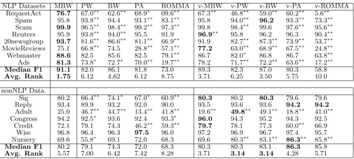
NLP Datasets MBW PW BW PA ROMMA v-MBW v-PW v-BW v-PA v-ROMMA RequestAct 76.7 67.0∗∗ 62.6∗∗ 68.9∗ 09.6∗∗ 67.3∗∗ 46.8∗∗ 59.0∗∗ 60.2∗∗ 5.6∗∗ Spam 95.8 93.8∗∗ 94.4 93.1∗∗ 83.1∗∗ 95.8 94.0∗∗ 96.2 93.3∗∗ 73.3∗∗ Scam 99.9 96.5∗∗ 98.4∗∗ 99.2∗∗ 97.3∗∗ 99.8 98.4∗∗ 99.6 97.6∗∗ 95.6∗∗ Reuters 95.9 93.8∗∗ 94.0∗∗ 95.5 91.9 96.9∗∗ 95.8 96.2 96.3 90.4∗∗ 20newsgroup 93.7 81.6∗∗ 86.6∗∗ 81.1∗∗ 66.9∗∗ 91.9 82.7∗∗ 87.3∗∗ 73.9∗∗ 53.7∗∗ MovieReviews 75.1 66.8∗∗ 74.5 28.8∗∗ 57.1∗∗ 77.2 63.0∗∗ 68.9∗∗ 67.5∗∗ 24.8∗∗ Webmaster 88.6 82.5 85.6 82.5 79.1∗∗ 86.7 82.0∗ 86.8 86.7 63.8∗∗ Ads 81.3 73.8∗ 72.7∗ 70.0∗∗ 19.7∗∗ 78.2 71.7∗∗ 72.2∗∗ 63.6∗∗ 17.2∗∗ Median F1 91.1 82.0 86.1 81.8 73.0 89.3 82.3 87.0 80.3 58.8 Avg. Rank 1.75 6.12 4.62 6.12 8.75 3.71 6.25 3.50 5.75 10.0 nonNLP Data. Sig 80.2 66.4∗∗ 74.1∗ 67.0∗ 60.9∗∗ 80.3 80.2 80.3 79.6 79.6 Reply 93.4 89.9 93.2 92.0 90.0 93.5 93.6 93.6 94.2 94.2 Adult 25.0 46.7∗∗ 44.7∗∗ 13.4∗∗ 41.8∗∗ 19.6∗∗ 49.8∗∗ 49.1∗∗ 18.8∗∗ 41.0∗∗ Congress 94.2 92.5∗ 93.6 92.4 93.3∗ 96.0 94.3 95.2 94.3 92.5 Credit 72.1 79.1 74.3 46.2∗∗ 59.3∗∗ 79.7 78.1 77.3 60.0∗∗ 66.9 Wisc 96.8 96.4 96.3 97.5 96.0 97.2 96.9 96.7 97.4 95.7 Nursery 69.6 55.8∗ 69.1 72.0 68.3 69.6 80.3∗∗ 83.1∗∗ 86.3∗∗ 85.8∗∗ Median F1 80.2 79.1 74.3 72.0 68.3 80.3 80.3 83.1 86.3 85.8 Avg. Rank 5.57 7.00 6.42 7.42 8.28 3.71 3.14 3.14 4.28 5.71
Table 3: General Performance of Single-Pass Online Learners – F1 measures (%). PW=Positive Winnow, BW=Balanced Winnow, PA=Passive-Aggressive. The symbols * and ** indicate paired t-Test statistical significance (relative to MBW) withp≤0.05and p≤0.01levels, respectively.
SVM v-P MBW v-MBW NB RequestAct 68.0 65.4 76.7 67.3 56.85 Spam 96.7 69.0 95.7 95.7 97.4 Scam 99.0 94.2 99.9 99.8 99.62 Reuters 96.7 96.3 95.9 96.8 85.52 20newsgroup 88.8 67.9 93.7 91.9 94.42 MovieReviews 78.5 71.4 75.1 77.1 71.85 Webmaster 88.9 88.5 88.6 86.6 77.38 Ads 80.5 58.0 81.3 78.2 52.5 Median F1 88.8 70.2 91.1 89.3 81.45 Avg. Rank 2.25 4.25 2.12 2.62 3.62 Signature 80.3 80.2 80.2 80.3 73.88 Reply-to 94.8 94.3 93.4 93.5 93.98 Adult 32.3 26.6 25.0 19.6 41.0 Congressional 96.2 95.7 94.2 95.9 91.7 Credit 80.2 59.5 72.1 79.6 66.78 WiscBreast 96.6 97.1 96.8 97.2 98.2 Nursery 87.1 86.8 57.0 69.6 84.4 Median F1 87.1 86.8 80.2 80.3 84.4 Avg. Rank 1.71 3.00 4.00 3.00 3.14
Table 4: General Performance - F1 measure (%). NB=Naive Bayes, v-P= Voted Perceptron.
ter (higher Median F1 and lower Avg. Rank) than non-voted Passive-Aggressive or non-voted ROMMA on both types of datasets. Passive-Aggressive typically presented better re-sults than ROMMA; and Balanced Winnow outperformed Positive Winnow in almost all tests. MBW outperformed all other online learners for NLP datasets, and also all other non-voted learners for non-NLP datasets.
We compare MBW results to the batch learners SVM and Naive Bayes in Table 4. This Table illustrates F1 results along with their standard errors for SVM, Voted Perceptron (or v-P), MBW, v-MBW and Naive Bayes (or NB) learners. Similar to Table 3, the datasets are presented in two groups (NLP and non-NLP) and best results are indicated in bold. From Tables 3 and 4, it is important to observe that the MBW learner indeed reaches impressive performance num-bers in the NLP-like datasets, outperforming all other
learn-ers — including SVM. The MBW performance in the NLP dataset is very encouraging, and a more detailed analysis of the behavior of this learner on NLP datasets will be pre-sented in Section??.
In the non-NLP tasks, however, SVM shows much better results than all other learners and MBW is not competitive at all. In fact, the Voted Perceptron would probably be the best choice for single-pass online learning in this type of data. It is interesting that the Voted Perceptron performs so well in non-NLP tasks and so poorly in NLP-like datasets.
In general, non-voted Winnow variants perform better in NLP-like than in non-NLP datasets. This agrees with the general intuition that multiplicative updates algorithms handle well high dimensional problems with sparse target weight vectors [11].
Table 3 also presents the overall effect of voting over the two types of datasets. It is easy to observe that voting im-proves the performance of all online learners for non-NLP datasets. However, for the NLP-like datasets, the improve-ments due to averaging are not as obvious. For instance, on Balanced Winnow, a small improvement can be observed, particularly when the F1 values are high. On Positive Win-now and Passive-Aggressive, it is not clear if voting is ben-eficial. For ROMMA, voting visibly deteriorates the formance. For MBW, voting seems to causes a small per-formance deterioration. It is not clear to the authors the reasons why averaging does not improve performance for NLP tasks in the single-pass setup.
In summary, voting seems to be a consistent and powerful way to boost the overall performance of very distinct single-pass online classifiers for non-NLP tasks. In NLP tasks, voting does not seem to bring the same benefits. More de-tailed experiments, learning curves and graphical analyses can be found in [6].
5. ONLINE FEATURE SELECTION
batch mode. Examples of common metrics for feature se-lection are Information Gain and Chi-Square [12, 22]. Ex-tending such batch feature selection techniques to the on-line learning setting is not obvious. In the onon-line setting the complete feature set is not known in advance. Also, it would be desirable to refine the model every time new examples are presented to the learner: not only by adding new meaningful features to the model, but also by deleting unimportant features that were previously selected. Adapt-ing the batch techniques to the online settAdapt-ing would be very expensive, since each score of each feature would need to be recalculated after every new example.
As previously seen, the MBW learner reaches very good performance in NLP tasks with a single learning pass through the training data. Here we propose a very simple and very fast online Feature Selection scheme called Ex-tremal Feature Selection (or EFS), based on the weights stored by the MBW learner. The idea is to rank the feature importance according to the difference (in absolute value) between its positive and negative MBW weights. More specifically, at each time t the importance score I of the featurejis given byItj= ˛ ˛uj t−v j t ˛ ˛whereuj t andv j t are the positive and the negative model weights for featurej.
After the scores Ij
t are computed, it would be expected that the largest values correspond to the most meaning-ful features to be selected at each time step. We would also expect that the lowest values ofIj
t correspond to the most unimportant features, prone to be deleted from the fi-nal model. In fact, a detailed afi-nalysis in the 20newsgroup dataset indicated that these low score features are typical stop words: e.g., “as”, “you”, “what”, and “they”.
In preliminary experiments, however, we observed an un-expected effect: performance is improved by selecting not only the highestIj
t-valued features, but also a small num-ber of features with the lowest values. EFS uses not only the extreme topT features, but also a small number from the extreme bottomB. For instance, in order to select 100 features from a dataset, EFS would select 90% of these 100 features from the extreme topT and 10% from the extreme bottomB.
The effectiveness of this idea can be seen in Figure 1. This figure illustrates the MBW test error rate for differ-ent numbers of features selected in the training set. More specifically, we first trained a MBW learner on the training set and then selected the features according toItj-values and P. We then deleted the other features (non-selected) from the MBW model and used this final model as test probe. We used a random split of 20% of the 20newsgroup data as the test set, and the remaining as training examples. The
quotient P = T
T+B represents the fraction of the selected features with high-scoreItj. For example,P= 0.7 indicates that 70% of the features were selected from the top and 30% from the bottom; andP = 1 indicates that no low-score fea-tures were selected at all.
As expected, the performances in Figure 1 improve as P
increases — since selecting more high score features trans-lates to better selection overall. This general behavior was also observed in all other NLP datasets. However, the con-dition P = 0.9 seems to outperform the condition P = 1, specially for non-aggressive feature selection (i.e., when the number of selected features is relatively large). This unex-pected behavior was also observed in other NLP datasets (see also Figure 2). It indicates that there is a small set
0 0.05 0.1 0.15 0.2 0.25 1 10 100 1000 10000 100000
Error Rate (on test set)
Number of Features Selected (from training set)
P=0.3 P=0.5 P=0.7 P=0.9 P=1.0
Figure 1: EFS experiment on the 20newsgroup dataset. P= T
T+B is the fraction of selected features
using highItj scores.
of low score features that are very effective to the proposed online feature selection scheme.
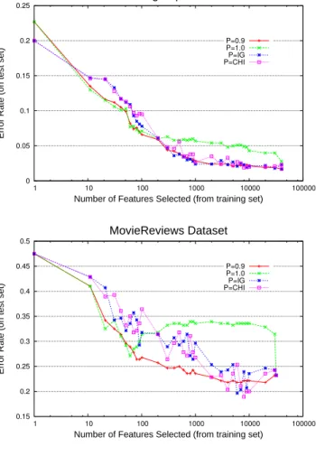
Similar to Figure 1, Figure 2 shows test error rates in other datasets for different numbers of features selected in the training set. Again, 20% of the data was used as the test set and the quotient P = T
K represents the fraction of the
selected features with high-scoreItj. Figure 2 also illustrates MBW performance using two popular batch feature selec-tion schemes: Informaselec-tion Gain (IG) and Chi-Square(CHI). For these two schemes, first a new training set containing only the selected features is created; then a MBW classifier learns a final model using the new training set.
Figure 2 reveals that EFS with P = 0.9 has a perfor-mance comparable to IG and CHI. In one of the experi-ments (MovieReviews) the EFS performance was generally better than IG or CHI in almost all feature selection ranges. Reuters was the only dataset where the traditional methods outperformed EFS, but only for very aggressive feature se-lection — when only a small number of features is selected. Additional experiments can be found in [6].
We speculate that the importance of these low score features is related to a smoothing-like effect in the MBW learner. Recall that MBW uses a normalization prepro-cessing step that is susceptible to the number of non-zero features in the incoming example, and the low-score features are frequently found in most examples. A more detailed investigation of this issue is a topic of future research. Another obvious future research will be applying such technique to other learning algorithms.
EFS results are very encouraging. The ability to perform effective online learning and feature selection in the same framework can largely benefit systems constrained by lim-ited resources.
6. ANALYSIS AND CONCLUSIONS
In this work we investigated the problem of single-pass on-line learning. This setting is particularly relevant when the system cannot afford several passes throughout the train-ing set—for instance, when dealtrain-ing with massive amounts of data, or when memory or processing resources are restricted. To the best of our knowledge, this is the first comprehensive
0 0.05 0.1 0.15 0.2 0.25 1 10 100 1000 10000 100000
Error Rate (on test set)
Number of Features Selected (from training set)
20newsgroup Dataset P=0.9 P=1.0 P=IG P=CHI 0.15 0.2 0.25 0.3 0.35 0.4 0.45 0.5 1 10 100 1000 10000 100000
Error Rate (on test set)
Number of Features Selected (from training set)
MovieReviews Dataset
P=0.9 P=1.0 P=IG P=CHI
Figure 2: EFS experiments: Comparison with In-formation Gain and Chi-Square.
comparison of online learners in the single-pass setting. We proposed a new modification of the Balanced Winnow algorithm (MBW) that performs surprisingly well in NLP tasks for the single-pass setting, with results comparable and sometimes even better than SVM. We evaluated the use of averaging (a.k.a. voting) on several online learners, and showed that it considerably improves performance for non-NLP tasks. Averaging techniques have been evaluated in the past for the Perceptron algorithm, but not for Winnow, Passive-Aggressive, ROMMA or other mistake-driven online learners.
Finally, we proposed a new online feature selection scheme based on the new MBW algorithm. This scheme is sim-ple, efficient, and naturally suited to the online setting. We showed that the method is comparable to traditional batch feature selection techniques such as information gain.
Acknowledgement
This material is based upon work supported by the Defense Advanced Research Projects Agency (DARPA). Any opin-ions, findings and conclusions or recommendations expressed in this material are those of the author(s) and do not nec-essarily reflect the views of the Defense Advanced Research Projects Agency (DARPA), or the Department of
Interior-National Business Center (DOI-NBC).
7. REFERENCES
[1] E. Airoldi, W. W. Cohen, and S. E. Fienberg. Bayesian methods for frequent terms in text: Models of contagion and the delta square statistic. InProceedings of the CSNA & INTERFACE Annual Meetings, 2005.
[2] E. M. Airoldi and B. Malin. Data mining challenges for electronic safety: The case of fraudulent intent detection in e-mails. InProceedings of the Workshop on Privacy and Security Aspects of Data Mining, pages 57–66. IEEE Computer Society, November 2004. Brighton, England. [3] R. Bekkerman, A. McCallum, and G. Huang. Categorization of
email into folders: Benchmark experiments on enron and sri corpora. Technical Report CIIR Technical Report IR-418, CIIR, University of Massachusetts, Amherst, 2004. [4] A. Blum. Empirical support for WINNOW and weighted
majority algorithms: results on a calendar scheduling domain. InICML, Lake Tahoe, California, 1995.
[5] V. R. Carvalho and W. W. Cohen. Learning to extract signature and reply lines from email. InProceedings of the Conference on Email and Anti-Spam, Palo Alto, CA, 2004. [6] V. R. Carvalho and W. W. Cohen. Notes on single-pass online
learning algorithms. Technical Report CMU-LTI-06-002, Carnegie Mellon University, Language Technologies Institute, 2006. Available from http://www.cs.cmu.edu/˜vitor. [7] C.-C. Chang and C.-J. Lin.LIBSVM: a library for support
vector machines, 2001. Software available at http://www.csie.ntu.edu.tw/˜cjlin/libsvm.
[8] W. Cohen, E. Minkov, and A. Tomasic. Learning to understand web site update requests. InIJCAI, Edinburgh, Scotland, 2005. [9] W. W. Cohen, V. R. Carvalho, and T. M. Mitchell. Learning to
classify email into “speech acts”. InEMNLP, pages 309–316, Barcelona, Spain, July 2004.
[10] K. Crammer, O. Dekel, S. Shalev-Shwartz, and Y. Singer. Online passive-aggressive algorithms. InNIPS, 2003. [11] I. Dagan, Y. Karov, and D. Roth. Mistake-driven learning in
text categorization. InEMNLP, pages 55–63, Aug 1997. [12] G. Forman. An extensive empirical study of feature selection
metrics for text classification.Journal of Machine Learning Research, 3:1289–1305, 2003.
[13] Y. Freund, Y. Mansour, and R. E. Schapire. Why averaging classifiers can protect against overfitting. InProceedings of the Eighth International Workshop on Artificial Intelligence and Statistics, 2001.
[14] Y. Freund and R. E. Schapire. Large margin classification using the perceptron algorithm.Machine Learning, 37(3):277–296, 1999.
[15] D. D. Lewis and M. Ringuette. A comparison of two learning algorithms for text categorization. InProceedings of SDAIR-94, 3rd Annual Symposium on Document Analysis and Information Retrieval, pages 81–93, Las Vegas, US, 1994. [16] Y. Li and P. M. Long. The relaxed online maximum margin
algorithm. InMachine Learning, volume 46, pages 361–387, 2002.
[17] N. Littlestone. Learning quickly when irrelevant attributes abound: A new linear-threshold algorithm.Machine Learning, 2(4), 1988.
[18] T. Mitchell.Machine Learning. Mcgraw-Hill, 1997. [19] K. Nigam, A. K. McCallum, S. Thrun, and T. Mitchell. Text
classification from labeled and unlabeled documents using EM. Machine Learning, 39((2/3)):1–32, 2000.
[20] B. Pang, L. Lee, and S. Vaithyanathan. Thumbs up? Sentiment classification using machine learning techniques. InEMNLP, 2002.
[21] F. Rosenblatt. The perceptron: A probabilistic model for information storage and organization in the brain. In Psychological Review, volume 4, pages 386–407, 1958. [22] Y. Yang and J. O. Pedersen. A comparative study on feature