Wayne State University Dissertations
1-1-2013
Essays On The Effects Of Oil Price Shocks On The U.s. Stock
Essays On The Effects Of Oil Price Shocks On The U.s. Stock
Returns
Returns
Zeina Nashaat Alsalman
Wayne State University, az0503@wayne.edu
Follow this and additional works at: https://digitalcommons.wayne.edu/oa_dissertations
Part of the Economics Commons, and the Oil, Gas, and Energy Commons Recommended Citation
Recommended Citation
Alsalman, Zeina Nashaat, "Essays On The Effects Of Oil Price Shocks On The U.s. Stock Returns" (2013). Wayne State University Dissertations. 828.
https://digitalcommons.wayne.edu/oa_dissertations/828
This Open Access Dissertation is brought to you for free and open access by DigitalCommons@WayneState. It has been accepted for inclusion in Wayne State University Dissertations by an authorized administrator of
ESSAYS ON THE EFFECTS OF OIL PRICE SHOCKS ON THE U.S.
STOCK RETURNS
by
ZEINA N. ALSALMAN
DISSERTATION
Submitted to the Graduate School
of Wayne State University,
Detroit, Michigan
in partial fulfillment of the requirements
for the degree of
DOCTOR OF PHILOSOPHY
2013
MAJOR: ECONOMICS
Approved by:
ZEINA N. ALSALMAN
AUGUST 2013
To my lovely family
My sincerest appreciation goes to my advisor, Ana Maria Herrera, for her patience, advice, and guidance throughout my research. She has added a lot to my professional progress. Professor Herrera was a friend when I needed one, always available with cheerful encouragement. I will always be grateful. My deepest thanks go to Professor Allen Goodman for his constant help, concern, and support during my studies. I am also deeply grateful to Dr. Robert J. Rossana, and Dr. Liang Hu for their critical comments and helpful suggestions. Special thanks goes to Dr. Li Way Lee for his encouragement and help.
Dedication...iii+ Acknowlegements ...iii+ List+of+Tables...vii+ List+of+Figures... ix+ Chapter+1:+Introduction ... 1+ Chapter+2:+Oil+Price+Shocks+and+the+U.S.+Stock+Market:+Do+Sign+and+Size+Matter? ... 6+ ++++++2.1+Introduction ... 7+ ++++++2.2+Data+Description... 12+ ++++++2.3+The+Effect+of+Oil+Price+Shocks+on+Stock+Returns... 15+ ++++++2.4+Does+the+Sign+of+the+Shock+Matter?... 17+ ++++++2.5+Does+the+Size+of+the+Shock+Matter?... 21+ ++++++2.6+The+Real+Price+of+Oil+versus+the+Nominal+Price+of+Oil ... 23+ ++++++2.7+Do+Oil+Prices+Help+Forecast+U.S.+Stock+Returns? ... 25+ ++++++2.8+Conclusions... 26+ Chapter+3:+Oil+Price+Uncertainty+and+the+U.S.+Stock+Market:+Analysis+Based+on+a+ +++GARCHWinWMean+VAR+Model... 39+ ++++++3.1.+Introduction ... 39+ JW
++++++3.3.+Methodology ... 47+ ++++++3.4.+Empirical+Results ... 50+ +++++++++++3.4.1+Oil+Uncertainty+Effect+on+the+U.S.+Aggregate+Stock+Returns... 51+ ++++++3.5.+Effect+of+Oil+Uncertainty+Across+Industries ... 54+ ++++++3.6.+Conclusions... 57+ Chapter+4:+Does+Uncertainty+in+Oil+Prices+Affect+U.S.+Stock+Returns?+Analysis+under+ the+Day+of+the+Week+Effect ... 70+ ++++++4.1+Introduction ... 71+ ++++++4.2+Data+Description+and+Model+Specification... 76+ ++++++4.3.+Empirical+Results ... 80+ ++++++++++4.3.1+Effect+of+Uncertainty+in+Oil+Prices+on+Aggregate+Stock+Returns ... 81+ ++++++4.4.+Effect+of+Oil+Uncertainty+Across+Industries ... 83+ ++++++4.5.+Conclusion... 87+ Chapter+5:+Research+Conclusions...100+ References...148+ Abstract...154+ Autobiographical+Statement ...156+ W
Table 2.1. Test of symmetry in the response to positive and negative innovations in the
real oil price for h = 1, 2, …, 12 ... 29+
Table 2.2. Direct and total requirements of crude petroleum and natural gas... 30+
Table 2.3. Test of symmetry in the response to positive and negative innovations in the nominal oil price for h = 1, 2, …, 12... 31+
Table 2.4. P-values for the test of null hypothesis of linearity of 12-month-ahead forecasts of real stock returns ... 32+
Table 3.1 Unit Root Test... 60+
Table 3.2 Summary Statistics ... 61+
Table 3.3 Skewness/Kurtosis Tests for Normality ... 62+
Table 3.4 Breusch-Godfrey LM test for autocorrelation ... 63+
Table 3.4.1 Engle's (1982) LM test for ARCH effects ... 64+
Table 3.5 LM tests for residual serial correlation... 65+
Table 3.6 LM tests for arch effects on the standardized residuals from the GARCH-in Mean ... 66+
Table 3.7 Model Specification Test... 67+
Table 3.8 Parameter Estimates for the Variance Function ... 67+
Table 3.9 Coefficient Estimates on Oil Volatility ... 68+
Table 4.1. Unit root test ... 90+
Table 4.2:Summary Statistics ... 91+
Table 4. 3. Coefficient Estimates on Oil Volatility ... 95+
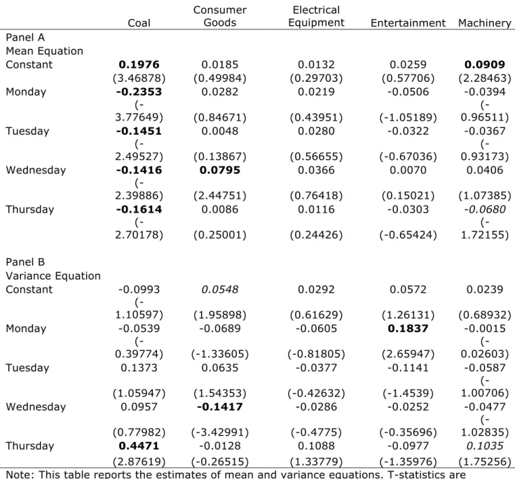
Table 4.4(a). Day of the week effect in the mean and variance equations ... 96+
Table 4.4(b).Day of the week effect in the mean and variance equations... 97+
Table 4.4(c).Day of the week effect in the mean and variance equations ... 98+
Table 2A: Standard Industrial Classification (SIC) Codes for Industries ... 104+
Figure 2.1(a-c): Response to one standard deviation positive and negative
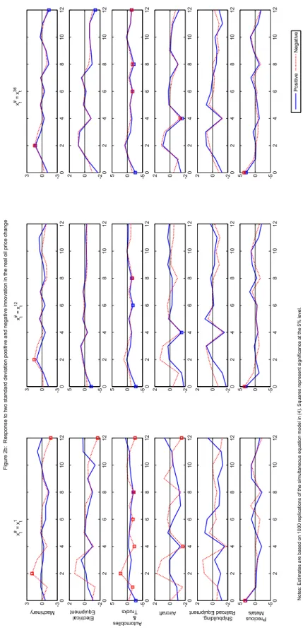
innovation in the real oil price change ………33 Figure 2.2(a-c): Response to two standard deviation positive and negative
innovation in the real oil price change ………36 Figure 3(a-c): Impulse response functions ……..……...………...69 Figure A.1 a-f: Response to one standard deviation positive and negative
innovation in the real oil price change …….……….118 Figure A.2 a-f: Response to two standard deviation positive and negative
innovation in the real oil price change ……….……….124 Figure A.3 a-i: Response to one standard deviation positive and negative
innovation in the nominal oil price change………...………130 Figure A.4 a-i: Response to two standard deviation positive and negative
innovation in the nominal oil price change……...………139
Chapter!1:!Introduction
Are energy price increases perceived to have larger effects than energy price decreases on the U.S. financial markets? Is the effect different between energy-intensive and non-intensive sectors? Does the size of the oil shock matters. This dissertation takes a fresh look at these questions using a conventional model proposed by Kilian and Vigfusson (2009). Since the 1970s, the macroeconomic literature has been testing for the oil price-macroeconomy relationship (see, e.g., Loungani (1986); Mork (1989); Lee, Ni and Ratti (1995); Hooker (1996); Hamilton (2010)), and questioning the symmetric responses of macroeconomic aggregates (see, e.g., by Kilian and Vigfusson (2009); Hamilton (2009); Herrera, Lagalo, and Wada (2010)), mainly after the major unanticipated falls in the price of oil, as appeared in 1986, 1998, and late 2008. On the other hand, the structural stability and functional form of the oil price-financial market relationship have been widely ignored in the literature. Although there are quite a few papers in the literature examining the impact of oil price changes on stock returns (see e.g. Ciner (2001); Basher and Sadorsky (2006); Cong et al. (2008); Park and Ratti (2008); Sadorsky (2008); Ramos and Veiga (2011); and Kilian and Park (2009)), none has directly tested for asymmetries in the transmission of oil price innovations to stock returns.
While stock market analysts and journalists have considered changes in oil prices as one of the main factors that explain instability in the stock market (see among others the Financial Times August 21, 2006, Wall Street Journal, August 8, 2008), there are still mixed evidence among academic researchers regarding the nature of the relationship between changes in crude oil prices and stock returns (see Chen, Roll & Ross (1986),
Jones & Kaul (1996) and Sadorsky (1999). Until recently, Kilian and Park (2009) show that the effect depends on the source of the shock. They show that the response of aggregate stock returns may differ greatly depending on whether the increase in the price of crude oil is driven by demand or supply shocks in the crude oil market. Thus, one explanation for the mixed results in the literature is that the source of the shock matters as shown in Kilian and Park (2009).
An alternative explanation for these contrasting results could stem from the asymmetry and possibly nonlinear nature of the relationship. If true, then the effect of an oil price shock on stock returns will depend on the size and the sign of the shock. In other words, agents respond differently to positive and negative oil price innovations, or firms’ stock returns react differently to the oil price increase that constitutes a correction for a previous decline than to an increase in a previously stable environment (Hamilton 1996, 2003).
Uncertainty and financial stress brought about by the oil price shock could explain why oil price shocks could have an asymmetric, and possibly nonlinear, effect on stock returns. Thus, using a bivariate GARCH-in-mean VAR model, this dissertation directly tests for the uncertainty effect of oil price changes on stock returns and whether the response of stock returns to an increase and a decrease in oil price volatility is symmetric. Moreover, considering seasonality in risk and returns is essential for financial managers and analysts. For instance, detecting a particular pattern in volatility might assist investors in making decisions based on both return and risk (Kiymaz and Berument, 2003). Thus, this dissertation examines the day-of-the-week effect in the crude oil market using GARCH models.
In addition, this dissertation characterizes the relationship between oil price changes and the U.S. stock returns not only at the aggregate level but also across sectors. Since results at the aggregate level might hide important effects of oil price volatility at the sectoral level, we examine the oil uncertainty effects on sectoral stock markets, and investigate whether the relationship between oil prices and sectoral stock returns is symmetric. Investigating the effect of oil price shocks at a sectoral level is important for a number of reasons. First, as we mentioned before, evidence regarding the presence (or absence) of asymmetry differs among sectors and in the aggregate (see Kilian and Vigfusson (2009) and Herrera et al (2010) for the oil price-macroeconomy relationship). Second, Fama and French (1997), among others, show that returns and volatility at the sectoral level offer important information about the return and volatility process at the aggregate level. Similarly, Hong et al. (2007) also recognize the importance of sectoral returns to give information about the movements of aggregate stock returns. Accordingly, it is important to examine the effect of oil price uncertainty on stock returns across industries especially during periods of instabilities in oil prices; so that investors can adjust their portfolios accordingly.
This dissertation is organized as follows, in chapter 2 we first inquire whether aggregate and industry-level stock returns respond to oil price shocks and then use state-of-the-art techniques to directly test for symmetry in the response to positive and negative real oil price innovations. We find no evidence of asymmetry for aggregate stock returns, and only very limited evidence at the sectoral level. We inquire whether the size of the shock matters in that doubling the size of the shock more (or less) than doubles the size of the response. Consistent with our finding that a linear model fits most of the industries,
we conclude that the effect of a 2.s.d innovation is just double the magnitude of the impact of a 1.s.d innovation. Furthermore, we find no support for the conjecture that shocks that exceed a threshold have an asymmetric effect on stock returns. We then explore whether our results are robust to specifying our model in terms of the nominal oil price. Our test results indicate a considerable increase in the number of rejections for the net oil price increase over the previous 12-month maximum, even after controlling for data mining.
Chapter 3 uses a bivariate GARCH–in-mean VAR model to examine the effect of oil price uncertainty on the U.S. real stock returns at the aggregate and sectoral level. Estimation results suggest that there is no statistically significant effect of oil price volatility on the U.S. stock returns. The absence of an uncertainty effect might be explained by the view that companies across sectors, the airline industry for instance, are likely to hedge against fluctuations in oil prices. It could also stem from the ability of most companies to transfer the higher cost of oil to customers. Moreover, the impulse responses indicate that oil price increases and decreases have symmetric effects on the U.S. stock returns, in that energy price increases and decreases are estimated to have equal and opposite effects on the U.S. financial market.
Using high frequency data, chapter 4 addresses the issue of uncertainty in oil prices and its effect on U.S. stock returns, taking into account the day of the week effect. The results suggest that the-day-of-the-week effect is present in both the mean and volatility equations. While the Wednesday dummy has a statistically significant effect on the conditional mean, Thursdays and Wednesdays appear to have the highest and the lowest aggregate returns volatilities, respectively. We also find that the U.S. stock market is
sensitive to oil price variations not only at the aggregate level but also across some industries, such as chemicals, entertainment, and retail, where uncertainty in oil prices proves to have positive and statistically significant effect. On the other hand, many sectors, such as transportation, automobiles, consumer goods, aircraft, and many others, came out to be unaffected by variations in oil prices.
Chapter 5 presents the contribution of this research to the literature of oil prices and stock returns. It also summarizes the major findings of this dissertation and suggests implications for future directions.
Chapter!2:!Oil!Price!Shocks!and!the!U.S.!Stock!Market:!Do!Sign!and!Size!
Matter?
1!
This paper investigates the effects of oil price innovations on the U.S. stock market using a model that nests symmetric and asymmetric responses to positive and negative oil price innovations. We first inquire whether aggregate and industry-level stock returns respond to oil price shocks and then use state-of-the-art techniques to directly test for symmetry in the response to positive and negative real oil price innovations. We find no evidence of asymmetry for aggregate stock returns, and only very limited evidence for the 49 industry-level portfolios studied in this paper. We inquire whether the size of the shock matters in that doubling the size of the shock more (or less) than doubles the size of the response. Consistent with our finding that a linear model fits most of the industries, we conclude that the effect of a 2.s.d innovation is just double the magnitude of the impact of a 1.s.d innovation. Furthermore, we find no support for the conjecture that shocks that exceed a threshold have an asymmetric effect on stock returns. We then explore whether our results are robust to specifying our model in terms of the nominal oil price. Our test results indicate a considerable increase in the number of rejections for the net oil price increase over the previous 12-month maximum, even after controlling for data mining. Do sign and size matter? The answer to this question appears to depend on whether the model is specified in terms of the real or the nominal price of oil.
2.1!Introduction!
Headlines such as "U.S. stocks plunge after oil climbs $6" (New York Times, June 11, 2008) or "U.S. stocks rally after crude drops to 3-month low" (Wall Street Journal, August 8, 2008) highlight the shared belief among journalists and stock market commentators that oil price shocks have a direct effect on U.S. stock markets. Moreover, these headlines put in evidence the belief that the effect might depend on the behavior of crude oil prices in the recent history.
For many years, researchers compiled conflicting evidence regarding the nature of the relationship between changes in crude oil prices and stock returns. On the one hand, Huang, Masulis and Stoll (1996) found no evidence of a negative relationship between prices of oil futures and stock returns. Similarly, Wei (2003) encountered that the oil price shock of 1973-74 had no impact on stock returns. On the other hand, work by Jones and Kaul (1996) pointed towards a negative effect of oil price shocks on stock returns. Yet, in recent years, a consensus appears to have emerged among academics: oil price shocks exert a negative impact on most stock returns, though the nature of the relationship depends on the underlying shock. In particular, Kilian and Park (2009) find that oil price shocks that are driven by innovations to the precautionary demand for crude oil have a negative impact on U.S. stock returns. They show that the response differs significantly depending on the source of the oil price shock (e.g., supply or demand driven). Thus, changes in the composition of oil price shocks over time help explain why, in the past, researchers failed to find evidence in favor of an effect of oil price innovations on U.S. stock returns.
An alternative explanation for these contrasting results could stem from the possibly nonlinear nature of the relationship. For instance, if people's perception of the importance of an oil price shock depends on the past history of oil prices (Hamilton 1996, 2003), or if firms' cash flows respond differently to positive and negative oil price innovations, then the effect of an oil price shock on stock returns will also depend on the size and the sign of the shock.
There are a number of reasons why oil price shocks could have an asymmetric, and possibly nonlinear, effect on stock returns. First, oil prices do not appear to have an asymmetric effect on aggregate real GDP (Kilian and Vigfusson 2011a) and aggregate industrial production (Herrera, Lagalo, and Wada 2011). Yet, they seem to have an asymmetric effect on some (but not all) industries that use energy intensively in their production process such as rubber and plastics, or in consumption such as transportation equipment (Herrera, Lagalo and Wada 2011). Asymmetries in the response of production could thus translate into an asymmetric response of profits and, thus, stock returns.
In addition, the optimal decision for a firm that pays dividends to its shareholders and seeks to maximize the expected present value of its dividends (without closing), could be to pay dividends only when its surplus exceeds a threshold (Wan 2007). Therefore, a negative (or a positive) oil price innovation could push the surplus below the cutoff required to pay dividends for an oil company (or an industry that uses energy intensively). If that is the case, the company could choose not to pay dividends and face a decline in stock prices. The negative impact that such a decision would have on stock returns is likely to be larger than the increase in stock returns that would stem from higher dividend payments due to a larger surplus.
Another possibility is that uncertainty and financial stress brought about by the oil price shock, could lead to asymmetries in the response of interest rates (Ferderer 1996; Balke, Brown and Yücel 2002). Such an effect would also be evident if people believed the monetary authority will respond differently to oil price increases and decreases. For instance, Ferderer (1996) and Bernanke, Gertler and Watson (1997) find that part of the decline in economic activity brought about by a positive oil price innovation can be attributed to a more restrictive monetary policy. Although the importance of this systematic monetary policy response --on average and after the Great Moderation-- is a question of debate (see, for instance, Hamilton and Herrera 2004, Herrera and Pesavento 2009, Kilian and Lewis 2010), one could conjecture that an asymmetric response of interest rates to oil price innovations could have an asymmetric effect on the expected present discounted value of the dividends and, thus, on stock returns.
These arguments merit careful investigations of the presence of possible asymmetries in the response of stock returns to unexpected variation in crude oil prices --both at the aggregate and disaggregate level. The contribution of this paper is threefold. First, we explore the question of asymmetry in the response of U.S. real stock returns. To do so we estimate a simultaneous equation model that nests symmetric and asymmetric responses to positive and negative oil price innovations using monthly data on aggregate US stock returns and 49 industry-level portfolios. We then employ state-of-the art techniques to directly test the null of symmetry in the response of real stock to real oil price innovations (see Kilian and Vigfusson 2011).
Our estimation results suggest the response of aggregate stock returns is well captured by a linear model. This is also the case for most of the 49 industry-level portfolios. Yet,
there are a number of portfolios (food products, candy& soda, beer and liquor, apparel, textiles, construction materials, automobiles and trucks, aircraft, communication, retail, banking, and insurance) where we find evidence of asymmetry. These results imply that financial investors interested in these industries should consider asymmetries in the response of stock returns to oil price innovations when forming their portfolios. Similarly, for financial forecasters, innovations of the same magnitude but opposite sign should not enter their loss function in a symmetric manner.
Second, we investigate whether the response of stock returns depends nonlinearly on the size of the shock. To do that, we evaluate whether the test of symmetry leads to different results when we consider innovations of one and two standard deviations. In addition, we explore whether only shocks that exceed a threshold have an asymmetric effect on stock returns as one could conjecture that agents chose to be inattentive to small oil price changes but re-optimize when changes are large.
Does the size of the shock matter? Consistent with our findings for the symmetry test, we conclude that for aggregate stock returns and for most industry-level portfolios the size of the shock matters only to the extent that it scales up the effect on stock returns. In addition, we show that a transformation of the oil price change that filters out movements that do not exceed one (or two) standard deviation(s) (as in Kilian and Park 2009) does considerably worse in fitting the data.
Third, we explore whether our findings regarding asymmetry (or the lack thereof) in the response of stock returns is robust to specifying our model in terms of the nominal price of oil. Even though theoretical models of the transmission of oil price shocks that imply an asymmetric response of economic activity are specified in terms of the real oil
price, it is conceivable that individuals and financial investors might choose to change their consumption or financial decisions when changes in the nominal oil price occur (Hamilton 2011). To explore this conjecture we specify our simultaneous equations model in terms of the nominal oil price and compute the test of symmetry in the response to positive and negative innovations in the nominal oil price.
We find ample evidence of asymmetry in the response to 1 s.d. innovation in the nominal price of oil, especially when we use the net oil price increase with respect to the previous 12-month maximum. In other words, while a linear model constitutes a good approximation to the relationship between real oil prices and real stock returns, a nonlinear model appears to provide a better description of the relationship between nominal oil prices and real stock returns. Hence, both the size and the sign matter when analyzing the effect of innovations in the nominal oil price.
Finally, we investigate whether oil price changes help forecast stock returns one year ahead. To do so, we compute the impulse response functions using local projection (Jordà 2005). We find evidence that the oil price increase, xt¹, helps forecast aggregate U.S. stock returns as well as industry-level returns one-year ahead. For automobiles and trucks, an industry that is commonly thought to be largely affected by oil price changes, we find that the oil price increase, xt1, and the net oil price increase relative to the
previous 36-month maximum, xt36, have predictive content. Of the four considered
non-linear oil price measures, oil price increases seem to do a better job at forecasting stock returns.
This paper is organized as follows. Section 2 describes the data on stock returns and oil prices. Section 3 explores the response of aggregate and industry-level stock returns to oil
price innovations. The results of the tests of symmetry in the response to a one standard deviation innovation (hereafter 1 s.d.) are reported in section 4. The following section explores whether our findings are robust to considering larger innovations (2 s.d.) or defining the nonlinear transformation in terms of oil price changes that exceed one or two standard deviations. Section 6 investigates the robustness of our results to specifying the model in terms of the nominal oil price. Section7 explores whether oil prices help forecast stock returns. Section 8 concludes.
2.2!Data!Description!
We use aggregate and industry-level U.S. real stock returns spanning the period between January 1973 and December 2009. Although data on stock returns and oil prices was available starting January 1947, we restrict the sample to the period between January 1973 and December 2009. This decision is motivated by the fact that oil prices behaved very differently during the years when the Texas Railroad Commission set production limits in the U.S. In fact, it was not until 1972 when U.S. production had increased significantly that nominal oil prices stopped being fixed for long periods of time2.
All of the data on monthly nominal stock returns were obtained from Kenneth French's database available on his webpage3. As a measure of aggregate stock returns we use the excess return on the market, which is defined as the value-weighted return on all NYSE, AMEX, and NASDAQ stocks from the Center for Research in Security Prices (CRSP) minus the one-month Treasury bill rate. For industry level stock returns we use the
2
Estimation results for the full sample are available from the authors upon request. 3
returns on 49 industry portfolios provided on French's webpage4. In this database each NYSE, AMEX, and NASDAQ stock is assigned to an industry portfolio based on its four-digit SIC code as reported by Compustat or, in absence of a Compustat code, by the four-digit SIC classification provided in CRSP. These portfolios include industries in agriculture, mining, construction, manufacturing, transportation and public utilities, wholesale and retail trade, finance, insurance and real estate, and services. (A complete list of the 4-digit SIC industries included in each portfolio is provided in the Appendix.) We then compute real stock returns by taking the log of the nominal stock returns and subtracting the CPI inflation.
Regarding the nominal oil price, we follow the bulk of the literature (see, for instance Mork 1989, Lee and Ni 2002) and use the composite refiners' acquisition cost (RAC) for crude oil from January 1974 until December 2009. Then, to compute prices for the previous months, we extrapolate using the rate of growth in the producer price index (PPI) for crude petroleum, after making adjustment to account for the price controls of the 1970s. The real price of oil is then computed by deflating the price of oil by the U.S. CPI.
To assess whether oil price innovations have an asymmetric effect on U.S. stock returns, we use three different nonlinear transformations of the real oil price, o_{t}. The first nonlinear transformation is a modified version of Mork's (1989) proposal to split percent changes in oil prices into increases and decreases to allow for an asymmetric response of aggregate production to positive and negative oil price shocks. That is, we use the oil price increase, which is defined as:
4+The data are available at: http://mba.tuck.dartmouth.edu/pages/faculty/ken.french/data_library.html. We use the file
xt¹=max(0,ln ot - ln ot-1). (1)
Alternatively, Hamilton (1996, 2003) suggests that agents might react in a different manner if the oil price increase constitutes a correction for a previous decline and not an increase in a previously stable environment. To account for this behavior, he proposes to use the net oil price increase as a measure of oil price shocks. Thus, as a second nonlinear transformation of oil prices we use the net oil price increase relative to the previous 12-month maximum (Hamilton 1996), which is given by:
xt¹²=max(0, ln ot - max(ln ot-1,..., ln ot-12)). (2)
The last measure is the net oil price increase over the previous 36-month maximum (Hamilton 2003), which is defined in a similar manner:
xt36=max(0, ln ot - max(ln ot-1,..., ln ot-36)). (3)
Although, the last two measures do not have a direct grounding on economic theory, there are behavioral explanations as to why agents might react differently in the face of a positive shock if oil prices have been stable in the near past or if they only represent a correction for a previous decline. In fact, the headlines reported in the news often suggest analysts and stock market commentators consider the behavior of oil prices in the recent past when thinking about the impact of shocks on stock returns.
2.3!The!Effect!of!Oil!Price!Shocks!on!Stock!Returns!
To evaluate the effect of positive and negative oil price innovations on stock returns we use a simultaneous equation model that nests both symmetric and asymmetric responses of stock returns. In addition, the nonlinear nature of this model allows for small and large oil price innovations to have different effects on the stock market. Thus, consider the data generating process for each of the stock return series, yi,t, to be given by
the following simultaneous equation model:
€ xt =a10+ a11,j j=1 12
∑
xt−j + a12,j j=1 12∑
yi,t−j+ε1t (4a) yi,t =a20+ a21,j j=0 12∑
xt−j+ a22,j j=1 12∑
yi,t−j+ g21,j j=0 12∑
xt#−j +ε2t (4b)where xt is the log growth of the crude oil price at time t, yt-j is the return on the the i-th
portfolio at time t, xt# is one of the nonlinear transformations of oil prices described in the
previous section, and ε1t and ε2t are, by construction, orthogonal disturbances. That is, for identification purposes, we assume that changes in oil prices have a contemporaneous effect on stock returns but stock returns do not affect oil prices contemporaneously. As for the number of lags included in the model, we follow Hamilton and Herrera (2004) in selecting twelve monthly lags to capture the effect of oil prices on economic activity.
Note that the inclusion of xt# in equation (4b) invalidates the computation of the
impulse response functions in the usual textbook manner (see Gallant, Rossi and Tauchen 1993 and Koop, Pesaran and Potter 1996). Instead, to compute the response of stock return i to an innovation of size δ in ε1t we use Monte Carlo integration. That is, we first calculate the impulse response functions to a positive innovation, Iy(h,δ,Ωt), and to a
negative innovation, Iy(h,-δ,Ωt) of size δ --conditional on the history Ωt-- for
h=0,1,2,...,12. We perform this computation for 1,000 different histories and then calculate the unconditional impulse response functions, Iy(h,-δ), by averaging over all the
histories5.
The first panel of Figure 1 illustrates the response of aggregate stock returns to positive and negative innovations of one standard deviation in the real oil price. For ease of comparison, we report the response to a positive innovation and the negative of the response to a negative innovation of size δ=1 s.d. Note that, regardless of the oil price measure, the effect of a 1 s.d. innovation in oil prices has a statistically insignificant effect on stock returns in the short-run. Using the oil price increase (the net oil price increase relative to the previous 36 months) the response of aggregate stock returns to both positive and negative innovations becomes significant at the 5% level 8 months (12 months) after the shock. In both cases, an unexpected increase in real oil prices leads to a decline in U.S. aggregate stock returns of less than 1%, whereas an unexpected decrease causes an increase of about the same magnitude. At a first sight, the fact that the IRFs to positive and negative innovations lie almost on top of each other suggests no asymmetry is present in the response of aggregate stock returns.
The remaining panels of Figure 1 plot the response of stock returns for a group of portfolios that are thought to be affected by oil prices (see Kilian and Park 2009). Evidence of a negative relationship between positive oil price innovations and real stock returns at the industry-level, for at least two of the oil price measures, is apparent for food products, candy and soda, beer and liquor, tobacco products, entertainment, printing and
5
See Herrera, Lagalo and Wada (2011) for a detailed description of the computation. +
publishing, consumer goods, apparel, medical equipment, pharmaceutical products, rubber and plastic products, textiles, construction materials, steel works, automobiles and trucks, aircraft, utilities, communication, personal services, computer hardware, electric equipment, measuring and control equipment, shipping containers, transportation, retail, restaurants, hotels, and motels, banking, insurance, real estate, and other. For most of these portfolios, the responses to positive and negative innovations of 1 s.d. lie on top of each other. This suggests that a negative innovation of 1 s.d. would have a positive effect on stock returns of the same magnitude but opposite sign.
These results are in line with Kling (1985) and Jones and Kaul (1996) who find a negative impact of oil price shocks on stock returns. Note that we find a statistically significant effect, even though we do not account for the source of the shock as in Kilian and Park (2009). In light of their result, one would expect the economic and statistical significance of oil price innovations to change over time depending on variations in the composition of the shock.
2.4!Does!the!Sign!of!the!Shock!Matter?!!
Recent research into the question of asymmetry in the response of economic activity to positive and negative oil price innovations suggests that the magnitude of the effect of a positive innovation is not larger (in absolute terms) than the magnitude of the effect of a negative innovation. Is this also the case for the response of U.S. stock returns? We address this question by implementing Kilian and Vigfusson's (2011) impulse response based test. That is, we use the impulse response functions computed in the previous section to construct a Wald test of the null hypothesis:
Iy(h,δ)=-Iy(h,-δ) for h=0,1,2,...,12.
Note that this test jointly evaluates whether the response of stock returns (for a particular portfolio) to a positive shock of size δ equals the negative of the response to a negative shock of the same size, -δ, for horizons h=0,1,2,...,12. Our motivation for focusing on a one-year horizon is twofold. First, the extant literature on the effect of oil price shocks has found that the largest and most significant impact on economic activity takes place around a year after the shock (see, for instance, Hamilton and Herrera 2004). Therefore, one could conjecture a similar lag in the transmission of oil price shocks to dividends, and thus to stock returns. But, even in the case where financial investors rapidly incorporate the information regarding oil price changes in their expected dividends, since the Wald test is a joint test for horizons h=0,1,2,...,12, we take into account the response at shorter horizons.
Second, by focusing on the 12-months horizon we avoid issues of data mining related to repeating the test over a different number of horizons. That is, if we were to repeat the impulse response based test with a 5% size say for 6 different horizons H, then the probability of finding at least one rejection would exceed 5% under the null.
Having addressed the possible issue of data mining across horizons by focusing on H=12, we still have to tackle data mining concerns related to repeating the impulse response based test over 49 different portfolios. To avoid this potential problem, we compute data-mining robust critical values by simulating the distribution of the supremum of the bootstrap test statistic, under the null, across all portfolios for each of
the oil price transformations6. To compute the data mining robust critical values we generate 100 pseudo-series using the estimated coefficient for the 49 portfolios in model (4). We then use 100 histories to get the conditional impulse response functions for each pseudo-series and compute the IRFs by Monte Carlo integration. We repeat this procedure 100 times to obtain the empirical distribution of the test statistic.
The left panel of Table 1 reports the p-values for the test of symmetry in the response to positive and negative innovations of 1 s.d in the real oil price. In addition we denote significance at the 5% and 10% level, after controlling for data mining, by ** and *, respectively. As the ‘eyeball metric’ would have suggested when looking at Figure 1, there is no evidence of asymmetry in the response of aggregate stock returns. Regardless of the oil price transformation (xt# =xt¹,xt¹²,xt³⁶), we are unable to reject the null at a 5%
level. As for the industry-level portfolios, we find some evidence of asymmetry when we use the oil price increase, xt¹, or the net oil price increase relative to the previous 12-month maximum, xt¹². In particular, using xt¹, we reject the null at a 5% significance level for candy & soda, apparel, textiles, construction materials, automobiles and trucks, communication, retail, and insurance. Note that these rejections are roughly consistent with what we would have obtained had we not controlled for data mining. When we use xt¹², we reject the null for food products, candy & soda, beer & liquor, aircraft, banking, and insurance. Interestingly, we fail to reject the null for all industry-level portfolios but insurance, when we use the net oil price increase with respect to the previous 36-month maximum, xt³⁶.
6
See Inoue and Kilian(2004) and Kilian and Vega (2010) for the effect of data mining and solutions to the problem of data mining in the related context of tests of predictability.
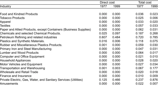
Finding asymmetries in the response of automobiles and trucks, aircraft, or apparel might not be surprising to the reader, as the use of transportation equipment requires considerable amounts of refined products and apparel is somewhat energy intensive in production (see Table 2). Thus, a-priori, one could expect the demand for these goods to contract more in response to positive oil price innovations than it would expand when faced by negative innovations. After all, firms might postpone the purchases of planes and individuals their purchases of cars when hit by an unexpected oil price surge, but they might not increase their demand when faced by an unexpected price drop. As a consequence, one would expect the response of profits, and thus stock returns, to be asymmetric. On the contrary, evidence of asymmetry in the food industries as well as in banking and insurance might be more puzzling as the total (direct and indirect) cost of crude petroleum and natural gas used to produce a dollar of output in these industries is less than 4 cents (see Table 2). A possible explanation for this finding could be that consumers increase precautionary savings when faced with a positive shock (Edelstein and Kilian 2009), reduce the demand for these goods, and this shortfall in demand leads to lower expected dividends and stock returns.
It is interesting to compare our results with those obtained by Herrera, Lagalo and Wada (2011) who study the question of asymmetry in the response of industrial production, as such a comparison could shed some light on the source of the asymmetry in stock returns. Using data mining robust critical values, they fail to reject the null of symmetry for H=12 for the total industrial production index, as well as for all the industry-level indices, when using xt¹ and xt¹². Instead, they find evidence of asymmetry in transit equipment, petroleum and coal, plastics and rubber, and machinery, when using
xt³⁶. In brief, there is no correspondence between our results and those for industrial production, which suggests that asymmetries in the response of industry-level stock returns are not driven by asymmetries in the response of production. Instead, other transmission mechanism influencing expectations of future dividends might be at play. Does the sign of the shock matter? For aggregate stock returns, the answer is only to the extent that the response has the opposite sign but not in the sense that positive and negative innovations have a symmetric effect. For most industry-level portfolio returns we find no evidence that positive innovations have a larger impact than negative innovations up to a year after the shock. Yet, there are a few industries where the sign of the shock matters in that the response of real stock returns is asymmetric.
2.5!Does!the!Size!of!the!Shock!Matter?!
In a linear model, the magnitude of the response to a 2 s.d. deviation shock is simply twice of the response to a 1 s.d. shock. Nevertheless, in a nonlinear model such as that in (4) the magnitude of the response depends on the size of the shock and on the history of oil price changes and stock returns. Thus, we estimate the IRFs to 2 s.d. innovations and test for symmetry in the response to positive and negative innovations of this magnitude, as we did in the previous section. The second panel of Table 1 reports the p-values for the test of symmetry in the response to a 2 s.d. innovation.
At first glance, it would appear that a doubling in the size of the innovation leads us to find more evidence of asymmetry. Note how there are more p-values below 5%, which are marked in bold, for a 2 s.d. innovation than for a 1 s.d. innovation. Yet, when we control for data mining, we find very little evidence of asymmetry. In fact, using xt¹ we
are unable to reject the null for the aggregate and all of the industry-level portfolios. For xt¹² we find evidence of asymmetry for candy & soda, coal, banking and insurance. The difference between the test results before and after controlling for data mining is indicative of the higher degree of uncertainty associated with the estimation of the IRFs to a 2 s.d. innovation. Moreover, since our data mining robust critical values are computed using the supremum of the bootstrap test statistic across all industry-level portfolios, it would suffice for the IRFs to be estimated with a higher degree of uncertainty for one portfolio in order to get larger critical values.
To further evaluate whether the size of the oil price shock matters, we consider a different oil price transformation along the lines of Edelstein and Kilian (2007). Consider a situation in which firms and individuals only respond to shocks that exceed a certain threshold. Such behavior could be observed if there are adjustment costs that prevent agents from optimizing when the change in the price of an input or a consumption good is small, or if dividends are paid only if the surplus exceeds a threshold.
Let us define € xtsd = 0 if |xt |≤δ xt if |xt |>δ $ % & ' ( ) (5)
where xt is the percentage change in the oil price, and δ equals one (4.45%) or two (9.9%)
standard deviations of the oil price change.
The fourth column of the left and right panels of Table 1 report the p-values for the test of symmetry computed using this alternative transformation of the oil price change. Clearly, there is no evidence of asymmetry in the response to 1 s.d. or 2 s.d. innovations when we use xtsd. In fact, our estimates suggest that xtsd does a very bad job at capturing
All in all, the response of aggregate stock returns to innovations in the real oil price, as well as that of most industry-level portfolios, is well captured by a linear model. Hence, the impact of innovations that differ only in size should differ only in the same scale. Yet, for a number of industries such as candy&soda, coal, banking, and insurance, the magnitude of the shock matters, as the response is a nonlinear function of the innovation.
2.6!The!Real!Price!of!Oil!versus!the!Nominal!Price!of!Oil!
Theoretical models that imply an asymmetric response of economic activity to oil price innovations are specified in terms of the real price of crude oil. However, Hamilton (2011) suggests that consumers of crude oil and refined products might respond to the nominal oil price, as it is more visible and readily available. Such a behavioral argument would seem to have more relevance for stock returns where financial investors could choose to buy or sell stocks in response to changes in the nominal crude oil price. To investigate whether our results are robust to the use of nominal oil prices, we specify model (4) in terms of the nominal oil price, estimate the impulse response functions to positive and negative innovations in the nominal oil price and compute the test of symmetry.
Table 3 reports the p-values for the test of symmetry in the response of stock returns to positive and negative nominal oil price innovations. In addition we denote significance at the 5% and 10% level, after controlling for data mining, by ** and *, respectively. As can be seen in first line of the table, the results for aggregate stock returns are unchanged. That is, whether we specify our simultaneous equation model in terms of the real oil price or the nominal oil price, a linear model appears to approximate well the effect of oil price
innovations on returns for the U.S. stock market. As for the industry-level portfolios, using xt¹ we reject the null of symmetry in the response to a 1 s.d. innovation for the same industries as we did using the real oil price. The only difference being that we now reject the null at a 5% level for real estate. Regarding the net oil price increase, evidence of asymmetry is more widespread when we use the nominal oil price, especially for the net oil price increase relative to the previous 12-month maximum. Note that for xt¹² (xt³⁶) we reject the null for 36 (6) of the 49 industry-level portfolios versus 6 (1) when we specified the model in terms of the real oil price. Similarly, for shocks that exceed one standard deviation, xtsd, the p-values are lower when we use the nominal oil price. The decrease is
such, that we are able to reject the null using the robust critical values for consumer goods and defense.
Comparing the right panels of Table 1 and Table 3 reveals only a slight increase in the number of rejections when we consider a 2 s.d. innovation. For instance, using xt¹ we reject the null for automobiles and trucks at a 5% level, whereas we obtained no rejections when we used the real oil price. Similarly for xt¹², we reject the null at a 5% significance level for computer software and at a 10% level for rubber and plastic products, and automobiles and trucks, in addition to the four portfolios where we found evidence of asymmetry to a 2 s.d. real oil price shock (candy&soda, coal, insurance and real estate). Here again, the fact that the number of rejections decreases considerably after controlling for data mining suggests an increase in the uncertainty involved in estimating the response to a 2 s.d. innovation.
All in all, our test suggest that the net oil price increase relative to the previous 12-month maximum, xt¹², does a better job than any of the other oil measures in capturing
possible asymmetries in the response of stock returns to positive and negative innovations. In particular, the fact that we reject the null of symmetry for a large number of industry-level portfolios suggests behavioral models of stock returns where financial investors respond to changes in the nominal oil price, but take into account the history of the price in the recent past are worth considering.
2.7!Do!Oil!Prices!Help!Forecast!U.S.!Stock!Returns?!
A related question is whether lagged oil price changes are helpful in forecasting U.S. stock returns. Hamilton (2011) suggests that a similar question -the predictive content of oil price changes for U.S. GDP growth-- can be addressed by computing the impulse response functions using local projections (Jordà's, 2005). Hence, we investigate whether non-linear measures of oil prices help predict U.S. stock returns h periods ahead. To do so we estimate the equation for forecasting stock returns h periods ahead directly by OLS
€ yi,t+h−1=α+ φj j=0 12
∑
xt−j+ βj 1 12∑
yi,t−j+ γj j=0 12∑
xt−# j +ut (6)and test the null hypothesis that lags of the non-linear measure of oil price, xt# , help
forecast U.S. stock returns: γ₁=γ₂=...=γ₁₂. As in the previous sections, we focus on the
one year horizon, h=12. We correct for serial correlation using Newey-West (1987) using 13 lags.
Table 4 reports the results for this test for each of the non-linear measures. Interestingly, we find evidence that the oil price increase, xt¹, helps forecast aggregate U.S. stock returns as well as industry-level returns one-year ahead. For 30 out of the 49 industry portfolios, as well as for aggregate returns, we can reject the null that the coefficients on current and lagged values of xt¹ are jointly equal to zero. Evidence that
other non-linear measures of oil prices help forecast stock returns is less widespread. First, we cannot reject the null for aggregate stock returns when we use xt¹²; xt³⁶; and xtsd.
Second, the number of industry-level portfolios where we are able to reject is lower: 19, 25 and 24, respectively.
Regardless of the oil price transformation, we reject the null for twelve industry-level portfolios: agriculture, recreation, entertainment, consumer goods, healthcare, medical equipment, pharmaceutical products, construction, electrical equipment, precious metal, mines, and computer software. As for automobiles and trucks, both the oil price increase, xt¹, and the net oil price increase relative to the previous 36-month maximum, xt³⁶, have a predictive content for one year ahead stock returns. Briefly, while only the oil price increase, xt¹, tends to predict aggregate U.S. stock returns one year ahead, the results are still mixed for industry-level returns.
2.8!Conclusions!
We started our study by inquiring whether the size and the sign of oil price shock matter for the response of U.S. real stock returns. To answer these questions we estimated a simultaneous equation model that nests symmetric and asymmetric responses to positive and negative innovations in the price of crude oil. We found that positive oil price innovations depress aggregate stock returns, as well as the returns of about 60% of the industry-level stock returns.
We explored the question of asymmetry in the response of real stock returns by implementing Kilian and Vigfusson's (2011) impulse response based test. To avoid issues of data mining related to the repetition of the test over all the portfolios, we bootstrapped
the distribution of the supremum of the Wald test across all portfolios. Estimation results suggested that a linear model fits the data well for aggregate returns, as well as for most industry-level portfolios. Notable exceptions are candy and soda, automobiles and trucks, and insurance for which we find evidence of asymmetry in the response to a 1 s.d. innovation using the oil price increase, xt¹, and the net oil price increase relative to the 12-month maximum, xt¹². No evidence of asymmetry is found when we use the net oil price increase relative to the 36-month maximum, xt³⁶. Consistent with these findings, we concluded that, for the aggregate and for most portfolios, the sign of the shock mattered only in that it determined the sign of the response. Yet, the absolute magnitude of the responses coincided.
To investigate whether the size of the shock matters we explored the question of symmetry in the response to a 2 s.d. innovation. For this larger shock, evidence of asymmetry was absent for all portfolios but candy and soda, coal, banking, and insurance, when we used xt¹². We then explored the conjecture that only oil price innovations that exceed a threshold (1 s.d. or 2 s.d. of the percentage change in the real oil price) have an asymmetric effect on real stock returns. Our estimation results lead us to strongly reject such a model. We thus concluded that the size of an innovation in real oil prices only matters in that it determines the scale of the effect. That is, consistent with our finding of symmetry, a doubling in the size of the innovation in real oil prices lead to a doubling (no more, no less) in the response of almost all analyzed stock returns.
Subsequently, we evaluated the robustness of our results to specifying the model in terms of the nominal, instead of the real oil price. Such a modeling choice could be grounded on a behavioral motivation along the lines of Hamilton (2011). That is, one
could surmise that financial agents react to changes in prices that are easily visible and thus stock returns respond to innovations in the nominal price of crude oil. Our test results implied a significant increase in the number of rejections, especially after controlling for data mining. In particular, we rejected the null of symmetry in the response to a 1 s.d. innovation for 36 of the 49 portfolios, when we used xt¹².
Finally, we examine whether oil price changes help forecast stock returns. Thus, we follow Hamilton (2011) and compute the impulse response functions using local projection (Jordà 2005). Results show that the oil price increase, xt¹, helps forecast aggregate U.S. stock returns as well as industry-level returns one-year ahead. Regarding an industry that is commonly thought to be most affected by oil price increases, automobiles and trucks, we find that only the oil price increase, xt¹, and the net oil price increase relative to the previous 36-month maximum, xt36, tend to forecast its returns
one-year ahead.
In brief, our results suggest a linear model provides a good approximation to the response of real stock returns to real oil price innovations. However, this is not the case when the model is specified in terms of the nominal price of crude oil. Do sign and size matter? The answer to this question appears to depend on whether the model is specified in terms of the real or the nominal price of oil.
Table 2.1. Test of symmetry in the response to positive and negative innovations in the real oil price for h = 1, 2, …, 12
Sector xt# = xt! xt# = xt12 xt# = xt36 xt# = xtsd xt# = xt! xt# = xt12 xt# = xt36 xt# = xtsd
Aggregate 0.34 0.76 0.73 1.00 0.35 0.51 0.84 1.00
Agriculture 0.48 0.72 0.61 1.00 0.56 0.14 0.93 1.00
Food Products 0.37 0.24** 0.64 0.99 0.57 0.03 0.87 1.00
Candy & Soda 0.04** 0.09** 0.45 1.00 0.01 0.00** 0.86 1.00
Beer & Liquor 0.48 0.20** 0.65 0.86 0.20 0.09 0.95 1.00
Tobacco Products 0.49 0.44 0.78 1.00 0.27 0.21 0.80 1.00
Recreation 0.29 0.57 0.66 1.00 0.28 0.36 0.90 1.00
Entertainment 0.20 0.45 0.55 0.99 0.07 0.17 0.74 1.00
Printing and Publishing 0.25 0.48 0.54 1.00 0.13 0.12 0.85 1.00
Consumer Goods 0.10* 0.31* 0.76 0.91 0.07 0.03 0.92 1.00 Apparel 0.01** 0.53 0.79 1.00 0.00 0.02 0.91 1.00 Healthcare 0.64 0.51 0.48 0.93 0.66 0.04 0.71 1.00 Medical Equipment 0.16 0.41 0.63 1.00 0.04 0.18 0.94 1.00 Pharmaceutical Products 0.36 0.40 0.88 0.99 0.15 0.25 0.96 1.00 Chemicals 0.57 0.63 0.62 1.00 0.56 0.21 0.84 1.00
Rubber and Plastic Products 0.25 0.70 0.92 1.00 0.22 0.06 0.93 1.00
Textiles 0.07** 0.57 0.69 1.00 0.02 0.01 0.77 1.00
Construction Materials 0.05** 0.29* 0.52 1.00 0.04 0.16 0.89 1.00
Construction 0.79 0.77 0.53 1.00 0.79 0.50 0.77 1.00
Steel Works Etc. 0.29 0.79 0.50 1.00 0.16 0.37 0.48 1.00
Fabricated Products 0.63 0.59 0.53 1.00 0.73 0.12 0.73 1.00
Machinery 0.47 0.66 0.59 1.00 0.49 0.19 0.71 1.00
Electrical Equipment 0.56 0.64 0.74 1.00 0.66 0.39 0.86 1.00
Automobiles and Trucks 0.01** 0.27* 0.79 1.00 0.00 0.03 0.71 1.00
Aircraft 0.16 0.18** 0.52 1.00 0.03 0.03 0.67 1.00
Shipbuilding, Railroad Equipment 0.10* 0.61 0.58 1.00 0.15 0.37 0.92 1.00
Defense 0.23 0.46 0.50 0.95 0.04 0.01 0.65 1.00
Precious Metals 0.93 0.50 0.41 0.93 0.97 0.05 0.71 1.00
Mines 0.58 0.92 0.89 1.00 0.43 0.80 0.89 1.00
Coal 0.77 0.57 0.42 1.00 0.75 0.00** 0.47 1.00
Petroleum and Natural Gas 0.94 0.81 0.76 1.00 0.94 0.24 0.74 1.00
Utilities 0.45 0.72 0.64 1.00 0.23 0.09 0.57 1.00 Communication 0.03** 0.80 0.68 1.00 0.01 0.36 0.79 1.00 Personal Services 0.52 0.57 0.46 1.00 0.34 0.19 0.85 1.00 Business Services 0.54 0.70 0.78 0.99 0.57 0.42 0.97 1.00 Computer Hardware 0.14 0.56 0.51 1.00 0.16 0.11 0.62 1.00 Computer Software 0.41 0.73 0.85 1.00 0.11 0.25 0.96 1.00 Electronic Equipment 0.10* 0.68 0.52 1.00 0.16 0.35 0.80 1.00
Measuring and Control Equipment 0.67 0.73 0.64 1.00 0.64 0.27 0.90 0.99
Business Supplies 0.35 0.32* 0.42 1.00 0.39 0.01 0.62 1.00
Shipping Containers 0.70 0.56 0.78 1.00 0.84 0.11 0.92 1.00
Transportation 0.29 0.38 0.35* 0.99 0.28 0.07 0.81 1.00
Wholesale 0.86 0.58 0.75 1.00 0.92 0.20 0.94 1.00
Retail 0.04** 0.84 0.77 1.00 0.00 0.43 0.92 1.00
Restaraunts, Hotels, Motels 0.46 0.59 0.79 1.00 0.24 0.23 0.94 1.00
Banking 0.12 0.08** 0.79 1.00 0.03 0.00** 0.79 1.00 Insurance 0.02** 0.06** 0.20** 1.00 0.00 0.00** 0.57 1.00 Real Estate 0.09* 0.47 0.68 1.00 0.01 0.01 0.87 1.00 Trading 0.36 0.62 0.94 1.00 0.47 0.04 0.92 1.00 Other 0.10* 0.31* 0.77 0.99 0.02 0.01 0.88 1.00 1sd 2sd
Notes: based on 1000 simulations of model (4). p-values are based on the "2
H+1 . Bold and italics denote significance at the 5% and 10% level,
Table 2.2. Direct and total requirements of crude petroleum and natural gas
Industry 1977 1999 1977 1999
Food and Kindred Products 0.000 0.000 0.036 0.023
Tobacco Products 0.000 0.000 0.025 0.006
Apparel 0.000 0.000 0.033 0.020
Textiles 0.000 0.000 0.057 0.033
Paper and Allied Products, except Containers (Business Supplies) 0.000 0.000 0.062 0.031
Chemicals and selected Chemical Products. 0.025 0.097 0.187 0.268
Petroleum Refining and related industries 0.607 0.484 0.720 0.785
Plastics and Synthetic Materials. 0.016 0.006 0.118 0.075
Rubber and Miscellaneous Plastics Products. 0.001 0.000 0.059 0.030
Primary Iron and Steel Manufacturing 0.000 0.000 0.047 0.031
Lumber and Wood Products 0.000 0.000 0.064 0.017
Computer and Office Equipment 0.000 0.000 0.021 0.010
Household Appliances 0.000 0.000 0.028 0.020
Motor Vehicles and Equipment 0.000 0.000 0.027 0.034
Transportation and Warehousing 0.001 0.003 0.067 0.177
Wholesale and Retail Trade 0.000 0.000 0.020 0.018
Finance and Insurance 0.000 0.000 0.010 0.009
Private Electric, Gas, Water, and Sanitary Services (Utilities) 0.125 0.466 0.237 0.876
Amusements 0.000 0.000 0.022 0.007
Direct cost Total cost
This table reports, as a measure of energy-intensity, total and direct costs of crude petroleum and natural gas required to produce a dollar of output of the particular industry in 1977 and 1999. These requirements are computed using the 1977 and 1999 annual Input-Output tables published by the BEA.
Table 2.3. Test of symmetry in the response to positive and negative innovations in the nominal oil price for h = 1, 2, …, 12
Sector xt# = xt! xt# = xt12 xt# = xt36 xt# = xtsd xt# = xt! xt# = xt12 xt# = xt36 xt# = xtsd
Aggregate 0.36 0.43 0.66 0.73 0.38 0.40 0.86 0.98
Agriculture 0.36 0.36 0.84 0.77 0.36 0.07 0.91 1.00
Food Products 0.40 0.08** 0.80 0.65 0.55 0.02 0.75 0.98
Candy & Soda 0.05** 0.00** 0.39 0.49 0.01 0.00** 0.72 1.00
Beer & Liquor 0.50 0.12** 0.65 0.43 0.16 0.12 0.89 1.00
Tobacco Products 0.55 0.12** 0.61 0.44 0.34 0.07 0.58 1.00
Recreation 0.32 0.15** 0.49 0.22 0.28 0.15 0.74 0.96
Entertainment 0.23 0.12** 0.57 0.36 0.08 0.09 0.76 0.87
Printing and Publishing 0.31 0.07** 0.60 0.46 0.14 0.02 0.88 1.00
Consumer Goods 0.14* 0.16** 0.30* 0.04** 0.08 0.05 0.72 0.92 Apparel 0.01** 0.14** 0.87 0.76 0.00 0.00 0.82 0.97 Healthcare 0.63 0.21** 0.24* 0.34 0.63 0.04 0.55 1.00 Medical Equipment 0.17 0.02** 0.59 0.57 0.04 0.04 0.84 0.97 Pharmaceutical Products 0.38 0.08** 0.58 0.57 0.14 0.11 0.87 0.99 Chemicals 0.61 0.21** 0.43 0.87 0.60 0.06 0.71 1.00
Rubber and Plastic Products 0.28 0.27* 0.75 0.31 0.24 0.03 0.77 0.91
Textiles 0.08** 0.18** 0.68 0.97 0.02 0.00* 0.56 0.99
Construction Materials 0.07** 0.07** 0.26* 0.56 0.06 0.04 0.66 1.00
Construction 0.80 0.31 0.79 0.87 0.81 0.35 0.78 0.98
Steel Works Etc. 0.33 0.27* 0.55 0.95 0.19 0.09 0.61 0.99
Fabricated Products 0.64 0.13** 0.60 0.94 0.72 0.03 0.72 0.95
Machinery 0.51 0.11** 0.61 0.57 0.55 0.03 0.82 0.95
Electrical Equipment 0.60 0.20** 0.88 0.85 0.70 0.19 0.86 0.98
Automobiles and Trucks 0.01** 0.06** 0.47 0.62 0.00** 0.00* 0.60 1.00
Aircraft 0.22 0.07** 0.09** 0.80 0.05 0.02 0.67 0.99
Shipbuilding, Railroad Equipment 0.12** 0.18** 0.79 0.81 0.16 0.16 0.72 0.98
Defense 0.27 0.39 0.24* 0.12** 0.05 0.02 0.28 0.72
Precious Metals 0.94 0.35 0.72 0.54 0.97 0.12 0.76 0.96
Mines 0.57 0.44 0.90 0.99 0.34 0.43 0.70 0.99
Coal 0.77 0.03** 0.30* 0.44 0.73 0.00** 0.37 0.91
Petroleum and Natural Gas 0.94 0.48 0.08** 0.97 0.93 0.31 0.51 0.95
Utilities 0.50 0.21** 0.44 0.83 0.26 0.01 0.27 1.00 Communication 0.04** 0.56 0.55 0.47 0.01 0.36 0.60 0.98 Personal Services 0.56 0.23* 0.38* 0.68 0.38 0.11 0.55 0.98 Business Services 0.59 0.13** 0.74 0.63 0.60 0.09 0.86 0.99 Computer Hardware 0.17 0.19** 0.51 0.28 0.20 0.04 0.70 0.94 Computer Software 0.49 0.06** 0.70 0.66 0.13 0.00** 0.87 0.95 Electronic Equipment 0.16* 0.18** 0.54 0.18* 0.24 0.08 0.86 0.81
Measuring and Control Equipment 0.76 0.19** 0.67 0.45 0.72 0.05 0.91 0.84
Business Supplies 0.45 0.10** 0.13** 0.62 0.47 0.01 0.44 1.00
Shipping Containers 0.66 0.23* 0.58 0.73 0.83 0.04 0.71 0.98
Transportation 0.25 0.05** 0.18** 0.65 0.26 0.01 0.71 0.96
Wholesale 0.88 0.13** 0.72 0.64 0.92 0.06 0.81 0.96
Retail 0.06** 0.57 0.91 0.87 0.00 0.32 0.85 0.99
Restaraunts, Hotels, Motels 0.51 0.11** 0.47 0.63 0.24 0.11 0.88 0.99
Banking 0.12** 0.01** 0.80 0.63 0.02 0.00** 0.59 0.99 Insurance 0.02** 0.00** 0.22* 0.79 0.00 0.00** 0.48 1.00 Real Estate 0.11** 0.26* 0.81 0.54 0.01 0.01 0.74 1.00 Trading 0.37 0.17** 0.93 0.57 0.48 0.01 0.90 1.00 Other 0.13* 0.03** 0.70 0.51 0.02 0.01 0.71 0.97 1sd 2sd
Notes: based on 1000 simulations of model (4). p-values are based on the "2
H+1 . Bold and italics denote significance at the 5% and 10% level, respectively.
Table 2.4. P-values for the test of null hypothesis of linearity of 12-month-ahead forecasts of real stock returns
Sector xt# = xt! xt# = xt12 xt# = xt36 xt # = x tsd Aggregate 0.00 0.11 0.26 0.12 Agriculture 0.00 0.00 0.00 0.00 Food Products 0.37 0.46 0.30 0.02
Candy & Soda 0.22 0.26 0.48 0.21
Beer & Liquor 0.38 0.29 0.95 0.03
Tobacco Products 0.00 0.12 0.00 0.02
Recreation 0.00 0.00 0.04 0.02
Entertainment 0.01 0.01 0.00 0.03
Printing and Publishing 0.26 0.07 0.01 0.16
Consumer Goods 0.00 0.04 0.05 0.10 Apparel 0.00 0.09 0.33 0.00 Healthcare 0.00 0.05 0.04 0.51 Medical Equipment 0.00 0.00 0.00 0.39 Pharmaceutical Products 0.00 0.01 0.03 0.02 Chemicals 0.02 0.16 0.09 0.02
Rubber and Plastic Products 0.00 0.60 0.35 0.12
Textiles 0.02 0.21 0.46 0.03
Construction Materials 0.04 0.23 0.53 0.04
Construction 0.00 0.00 0.00 0.06
Steel Works Etc. 0.00 0.41 0.31 0.08
Fabricated Products 0.00 0.07 0.05 0.30
Machinery 0.00 0.03 0.11 0.10
Electrical Equipment 0.03 0.02 0.00 0.01
Automobiles and Trucks 0.02 0.27 0.03 0.06
Aircraft 0.31 0.61 0.38 0.00
Shipbuilding, Railroad Equipment 0.36 0.57 0.65 0.05
Defense 0.33 0.42 0.06 0.05
Precious Metals 0.00 0.01 0.00 0.06
Mines 0.00 0.00 0.00 0.01
Coal 0.00 0.08 0.77 0.48
Petroleum and Natural Gas 0.57 0.21 0.61 0.03
Utilities 0.00 0.49 0.93 0.88 Communication 0.32 0.26 0.00 0.00 Personal Services 0.12 0.01 0.00 0.01 Business Services 0.16 0.53 0.21 0.04 Computer Hardware 0.34 0.01 0.03 0.10 Computer Software 0.00 0.05 0.00 0.60 Electronic Equipment 0.11 0.01 0.02 0.06
Measuring and Control Equipment 0.02 0.07 0.04 0.18
Business Supplies 0.07 0.02 0.21 0.01
Shipping Containers 0.10 0.01 0.07 0.00
Transportation 0.10 0.06 0.02 0.04
Wholesale 0.03 0.06 0.03 0.34
Retail 0.01 0.13 0.01 0.06
Restaraunts, Hotels, Motels 0.00 0.13 0.29 0.00
Banking 0.02 0.34 0.05 0.22
Insurance 0.07 0.02 0.01 0.16
Real Estate 0.33 0.07 0.08 0.06
Trading 0.09 0.49 0.46 0.09
Other 0.00 0.04 0.33 0.10
Figure 2.1(a-c): Response to one standard deviation positive and negative innovation in the real oil price change
! " # $ % &! &" '" ! " ()) *+ ),-+ ! " # $ % &! &" '" ! " ! " # $ % &! &" '" ! " ! " # $ % &! &" '" ! " ./-+ *-, 0/1+ /-! " # $ % &! &" '" ! " ! " # $ % &! &" '" ! " ! " # $ % &! &" '" ! " 23/ 451+ * 8466 6733 ! " # $ % &! &" '" ! " ! " # $ % &! &" '" ! " ! " # $ % &! &" '" ! " 29+ 10:, ;4 ! " # $ % &! &" '" ! " ! " # $ % &! &" '" ! " ! " # $ % &! &" '" ! " <5= =+* 6>6? ;,4 -0: -46666666 85: 6?*3 ! " # $ % &! &" '" ! " ! " # $ % &! &" '" ! " ! " # $ % &! &" '" ! " @-+ +;6A 3*B 4 6.-: C666666 ! " # $ % &! &" '" ! " ! " # $ % &! &" '" ! " 6 6 ?340-0D+ E+),-0D+ F0)5*+6&,G66<+4H3/4+6-363/+64-,/8,*868+D0,-03/6H340-0D+6,/86/+),-0D+60//3D,-03/60/6-9+6*+,;630;6H*0:+6 :9,/)+ E3-+4G6 .4-01,-+46,*+6=,4+863/6&!!!6*+H;0:,-03/463I6-9+64015;-,/+3546+J5,-03/6138+;60/6K#LC6@J5,*+46*+H*+4+/-640)/0I0:,/:+6,-6-9+6MN6;+D+;C O -P6Q6O -& O -P6Q6O -R$ O -P6Q6O -&"
Figure 2.1(a-c): Response to one standard deviation positive and negative innovation in the real oil pr