Chicken or egg: financial development and economic growth in China, 1992-2004

CCSO Centre for Economic Research

University of Groningen

CCSO Working Papers

December, 2005

CCSO Working paper 2005/09

Chicken or egg: Financial development and economic growth in

China, 1992-2004

Xuejun Fan

Finance Department, Business School East China Normal University

Jan Jacobs

CCSO and Faculty of Economics, University of Groningen

Robert Lensink

Faculty of Economics, University of Groningen

CCSO Working Papers http://www.eco.rug.nl/ccso

Chicken or Egg: Financial Development and Economic Growth in

China, 1992-2004

Xuejun Fan

, Jan Jacobs

and Robert Lensink

1

Finance Department Business School East China Normal University 3663 North Zhong-shan Road 200062 Shanghai, P.R.China 2

CCSO and Faculty of Economics University of Groningen PO Box 800, 9700 AV Groningen The Netherlands 3 Faculty of Economics University of Groningen PO Box 800, 9700 AV Groningen The Netherlands [[email protected]]

December 2005

This paper contributes to the empirical finance-growth literature by examining the relationship between financial depth, banking sector development, stock market development and economic growth in China. After an extensive survey on recent financial reforms in China, we apply Granger (non-)causality tests for non-stationary variables to examine long-run and short-run causality between economic growth and financial development. We find positive relationships between financial depth, banking sector development and growth. However, stock market development does not seem to have a positive effect on long-run economic growth.

Keywords Financial development, economic growth, China, Granger (non-)causality tests, non-stationary variables

JEL Classifications O16, C44

Acknowledgements

1. Introduction

Whether financial development influences economic growth is a crucial policy issue. It is therefore no surprise that the importance of financial development for economic growth has been the focus of the theoretical debate for a long time. Already in the 1930s Schumpeter (1939) underlined the important role of financial intermediaries in screening investments and improving the marginal productivity of capital. Some decades later, Gurley and Shaw (1955; 1960) argued that financial intermediation increases the amount of funds available for investment by mobilizing saving and providing credit through financial intermediaries. Also Goldsmith (1969) pointed out that financial intermediation is related to economic growth.

The early models on financial intermediation and economic growth lacked solid modeling of the exact mechanisms of the relationship between the two variables. In the 1990s many new theoretical contributions on how financial intermediation may affect economic growth emerged. Examples are Greenwood and Jovanovic (1990), Bencivenga and Smith (1991, 1993), Obstfeld (1994) and Sain-Paul (1992). The wave of new theoretical models on the relationship between financial development and economic growth has triggered new empirical interest into the relationship between finance and growth. Some well-known examples are Atje and Jovanovic (1993), Berthelemy and Varoudakis (1996), King and Levine (1993abc), Levine and Zervos (1998), Levine et al. (2000) and Beck et al. (2000). See also Levine (1997) for an extensive survey of the literature until the mid 1990s.

In the majority of these papers a similar type of methodology is used. Mostly, a proxy for economic growth is regressed on a huge amount of possible determinants,

including financial indicators. The methodology that is used accords with the so-called Barro (1991) growth regressions. The studies by King and Levine (1993b) and Levine and Zervos (1998) are noteworthy. King and Levine (1993b) find that

financial development, in general and in terms of the development of banks, has a positive and robust impact on economic growth for a group of 80 countries over the 1960-1989 period. Levine and Zervos (1998) provide strong evidence for a positive and robust effect of equity market development on the growth indicators. Levine et al. (2000) and Beck et al. (2000) differ from the other studies in that they more seriously deal with simultaneity and unobserved country-specific effects by using a GMM estimation technique. In addition, they present cross-sectional instrumental variable estimators where legal rights of creditors are used as instruments. These studies are in line with the other studies mentioned above in that they also provide empirical

evidence for the growth-enhancing hypothesis of financial development.

The majority of the panel and cross-country studies on financial development and economic growth find that financial development has a positive effect on economic growth. These studies also provide some empirical evidence for the hypothesis that it is the overall provision of financial services (banks and financial markets taken together) that is important, and not whether a country has a bank-based or a market-based financial system. However, the cross-country type of studies is not without problems, since they do not properly account for the time dimension. Moreover, the cross-country estimates can give a wrong impression of the impact of financial

development on economic growth since they assume that the different countries in the model are homogeneous entities. Since countries may differ greatly with respect to institutions and economic policies used, results may be country specific. It is also

argued that while the cross-country type of studies may give some evidence for a positive correlation between income per capita and the development of the financial sector, the causality between financial sector development and economic growth remains unclear. Most of the multi-country studies do not pay much attention to the direction of causality. They seem to implicitly assume that financial development causes economic growth, in line with the supply-leading view (Patrick, 1966). However, financial development may also be demand-driven (see Saint-Paul, 1996). In addition, there may be a two-way causation where on the one hand growth

stimulates the creation and growth of financial intermediaries, whereas on the other hand these intermediaries contribute to higher growth (for a theoretical model, see Greenwood and Jovanovic, 1990).

Recently, some studies emerged in which it is tried to come around the above-mentioned problems. In these studies, explicit attention is given both to the question whether sample countries can be pooled and to the time series properties of the data. Moreover, Johansen’s (1988, 1991) method based on vector error-correction

mechanisms (ECM) is used to test for long-run cointegration between financial development and economic growth. This methodology allows formal testing of short-run and long-short-run causality between finance and growth. Some well-known examples are Demetriades and Hussein (1996), Arestis and Demitriades (1997), Arestis et al.

(2001) and Arestis et al. (2004). By specifying and estimating models for individual countries these studies show that results are country specific. The studies deny that financial sector development in general is a determining factor for the process of economic development. It appears that in some countries finance affects growth, while in other countries growth determines finance or the causality is twofold. Most

importantly, these studies argue that generalizations based on multi-country results may lead to incorrect advices at the country level. Some studies use a similar methodology for heterogeneous panels. A recent example is Christopoulos and Tsionas (2004). They estimate an error correction model for a panel of 10 countries and find that long run causality runs from financial development to growth, which contradicts the single country studies by e.g. Arestis et al. (1997, 2001).

The short survey presented above clearly shows that the relationship between

financial development and economic growth is still ambiguous, and country specific. Thus, it is by no means universal that financial development can contribute to

economic growth. Moreover, there is still a theoretical debate on the relative

importance of banking sector development versus stock market development. Several authors strongly question the importance of stock market development for long-run economic growth (see e.g. Singh, 1997). In this paper, we contribute to the empirical finance-growth literature by examining the causal relationship between financial development and economic growth for China. In our view, it is highly interesting to focus on China. China is currently one of the most important countries in the world. It has the largest population of any country, about 1.26 billion people in 1999 (Allen et al., 2002). Moreover, China’s GNP in terms of US$ is the seventh in the world, and its average growth rate (8.4% during the 1990-1998 period) is among the highest in the world. Allen et al. (2002) even argue that it will only take 15 years before China will become the largest economy in the world, if Purchasing Power Parity GNPs are used. China’s financial system is still state-controlled and bank-dominated. However, since the market-oriented economic reforms in 1978, China started a process of financial deregulation and liberalization, which led to a steady growth of the financial

sector. Moreover, since the beginning of the 1990s, China opened two stock markets, the Shanghai and ShenZhen Stock Exchanges, in 1990 and 1991, respectively. While the banking sector is still more important, the stock markets are growing very fast. For China it is a crucial policy issue to know to what extent its policy of financial

deregulation and the implied growth of the financial sector have contributed to economic growth. In addition, given the fast growing stock exchanges, more

information on the importance of equity markets vis-à-vis the banking sector for long-run economic growth in China is indispensable.1

The paper has some special features. First, we focus on a single country, China, to come around the problem that results may be country-specific. This may especially be the case for China, since China’s development differs considerably from most other emerging economies. In China the legal and the financial system are still relatively underdeveloped, although it is one of the fastest growing economies in the world (Allen, et al. 2000). Second, we use unit root tests to examine the time series

properties of the data. Third, we use Granger (non-)causality tests for non-stationary variables. Fourth, we explicitly consider short and long-run causality by specifying, estimating and formally identifying a vector error correction model (VECM). Finally, we pay attention to the impact of financial depth, the development of the banking sector and the development of the stock markets. To the best of our knowledge, this is the first study that has used Granger (non-)causality tests for non-stationary variables

1

The role and contribution of the equity markets in China is heavily discussed. Some economists are positive about the role of stock markets in China. See e.g. Xiang (1998) and Li (1994). Others, are more pessimistic about the stock markets contribution in general (Singh, 1997), or for China (Laurenceson, 2002).

to rigorously examine long run relationships and causality between economic growth, financial depth, bank development and the development of stock markets for China.

The remainder of this paper is organized as follows. Section 2 presents a survey of recent financial reforms in China. Section 3 presents our methodology. After the description of our data in Section 4, Section 5 presents the regression results. Section 6 summarizes the paper and outlines some areas of further research.

2. Financial Reforms in China

This section gives an overview of financial reforms in China during the last decades. It serves as background information for the main analysis in this paper, the long-run relationships between financial development and economic growth.

Before the financial reforms started, the government in China heavily controlled the banking sector and a stock market did not exist. Financial policy could be described as a policy of financial repression. The interest rate structure was distorted due to interest rate controls, banks were subject to excess taxation, and credit was allocated bureaucratically to preferred end users, notably state-owned companies. Moreover, the entry of new banks was under strict central government control. The economic reforms in China from 1978 onwards, however, changed financial policy gradually from financial repression to financial liberalization.

Reforms in the banking sector

The development of China’s banking sector has experienced the following phases.2

1979-1993: Establishment of a two-tier banking system

Before the reforms, China had a mono-banking system in which one institution, the People’s Bank of China, acted as China’s central bank and the sole deposit taking and lending institution. This structure began to change in 1979, when the Agriculture Bank of China, the Bank of China and the Construction Bank were established as state-owned specialized banks. More importantly, in 1984 the State Council

designated the People’s Bank of China (PBC) to be the central bank, and established the Industrial and Commercial Bank, the fourth state-owned specialized bank, to take over the deposit taking and lending functions of the People’s Bank of China.

Starting in 1984, selected new banks were permitted to operate alongside the four specialized banks. During the second half of the 1980’s, a flourishing network of nonbank financial institutions (NBFIs) such as trust and investment companies, urban credit cooperatives, and finance companies emerged.

1994-1997: Commercialization and Central Bank Independence

In 1994 three policy banks were established to take up the policy-directed lending activities of specialized banks in order to transfer the specialized state banks into real commercial banks. The new Commercial Bank Law that came into effect in 1995 restricted the banking businesses of commercial banks to deposit taking and loan

2_{This paragraph is based on Li (2001), Mehran and Quintyn (1996), Shirai (2001),}

Bhattasali (2002), Liu (2002), Laurenceson (2002), Green (2003a,b), and Shirai (2002).

extension in order to separate commercial banking from investment banking business, and also contained measures to improve managerial profit incentives and the quality of bank loan portfolios.

Although the PBC was formally entrusted with central banking functions in 1984, its control over the money supply was weak. The new PBC Law of 1995 gave the PBC the legal foundation to perform the central bank functions of monetary policy,

management and supervision of the financial institutions under the leadership of state council, without other government agencies or ministries interfering any more. The law also ended PBC financing of the fiscal deficit.

In January 1996, a new national unified inter-bank market is opened in Shanghai. Access to the market is restricted to the national headquarters of specialized banks and PBC branches in 35 cities. Inter-bank lending is limited to short-term transactions (maximum of four months).Other financial institutions such as the headquarters of national and regional commercial banks as well as Urban Cooperative Banks in principle also have access to the national interbank market. It is noteworthy that by mid-1996, interest rates in the short term and the interbank markets had been fully liberalized. Moreover, in 1994 credit ceilings on financial institutions other than specialized banks were eliminated and replaced by asset and liability regulations.

1998-2001: The management of NPLs and financial sector restructure

Since the currency crisis of the East Asian countries in 1997, Chinese authorities have seriously been alarmed by a large amount of non-performing loans (NPLs) in the banking system. Therefore, in 1998 270 billion RMB was injected into the four state-owned commercial banks in order to re-capitalize. In addition, in November 2001

PBC approved the merger of 1,658 rural credit cooperatives into 81 joint stock city

and rural commercial banks in accordance with the assessment of assets and capital,

write-off of some bad debts, and encouragement of new shareholders. This is part of a pilot reform of the rural financial system. Other reform measures in this period

include the closure and bankruptcy of insolvent financial institutions. The Hainan Development Bank and three trust and investment companies that had become highly insolvent were closed in 1997-1998.

2002-: Opening of financial industryand privatization

After China’s accession to WTO, its banking sector has been gradually opened. In addition, foreign currency business is more and more allowed without geographical and client restrictions. China’s commitments to fully open the sector to foreign competition by December 2006 as part of the WTO agreement increases the urgency of restructuring the major banks. In December 2003 the Chinese government

announced the recapitalization of the Bank of China and China Construction Bank. More importantly, the regulatory authorities have put in place performance targets and guidelines for reforming corporate governance in these two banks to ensure that balance sheets are further strengthened. Efforts now focus on rapidly restructuring these banks and encouraging them to list on the stock exchange,

Reforms of stock markets

The development of China’s stock market is one of the most important elements of China’s reform of the financial system. In December 1990 and July 1991 two stock markets, the Shanghai Stock Exchange (SSE) and the Shenzhen Stock Exchange (SZSE) were established. In China there are two main types of shares: A shares and B

shares. A shares are exclusively sold to Chinese nationals. B shares are traded in foreign currencies by foreign investors. Since February 2001, domestic investors are also allowed to buy B shares. In addition to the A and B shares, Chinese companies can issue H shares on the Hong Kong Stock Exchange, N shares on the New York Stock Exchange and S shares on the Singapore Stock Exchange.

China’s stock market has experienced an amazing growth. Initially, there were only eight companies listed on the Shanghai Stock Exchange and six on the Shenzhen Stock Exchange. In the beginning of the 1990s, the stock markets grew largely because of promotion by local government bodies in Shanghai and Shenzhen. The central government did not pay attention to stock market reforms. However, from 1996 onwards, the central government began to pay considerable attention to the development of stock markets. In 1997, the Government even endorsed a plan to transform more than 10,000 SOEs into publicly listed companies. By the end of 2003, about 1287 companies are listed on the two stock exchanges. These enterprises raised RMB 998.26 billion from the stock markets. On June 25, 2004 China launched a new small-company stock market in Shenzhen.

3. Methodology

Section 2 clearly suggests that China experienced a rapid financial development, in terms of financial depth, banking sector development and stock market growth. An important question is whether this financial development positively affects economic growth in the long run, or whether the relationship runs from growth to finance. In the remainder of this paper we will try to shed some light on this important policy issue

by applying a Granger (non-)causality analysis. Before presenting the analysis, this section explains our methodology in detail.

Granger (non-)causality analysis for non-stationary time series

We will use Granger (non-)causality analysis to provide empirical evidence on the question of causality between finance and growth. The basic principle of Granger (non-) causality analysis is to test whether or not lagged values of one variable help to improve the explanation of another variable from its own past. To analyse Granger (non-)causality between our variables, we set up a Vector AutoRegression (VAR) system for the n-vector zt

t t t A L z e

z = ( ) ₋₁+ , (1)

where A(L) is a matrix polynomial in the lag operator L(Lz_t =z_t−1)of degree p,

p pL A L A L A L A = + 2 +K+ 2 1 )

( , and etis an error term. The null hypothesis of noncausality from the first variable, say, of vector zt to the other variables in vector z can be formulated in terms of restrictions on the matrices A,, in particular the first element in the second row of all Ai matrices need to be equal to zero. Defining z1t as

the first element of z_t and z_2t as the other elements and introducing conformable partitioning of relevant vectors and matrices as

, 2 1       = t t t z z z , 22 , 12 , 21 , 11 ,       = i i i i i A A A A A i₌1,K,p_{, and ,} 2 1       = t t t e e e

the null hypothesis of noncausality from z1t to z2t is

. 0 21 , 21 , 2 21 , 1 = A = = Ap = A K

The conventional Granger (non-)causality test in a VAR system assumes stationarity. If the time series are not stationary, the stability condition for the VAR is not met, implying that Wald test statistics for Granger (non-)causality are invalid. To investigate causal relationships between non-stationary variables the cointegration approach and vector error correction models (VECM) are recommended (Toda and Phillips, 1993, 1994). According to Engle and Granger (1987) two or more non-stationary variables are said to be cointegrated if there exists a linear combination that is stationary. They have also formally proven the correspondence between

cointegration and error-correction mechanism. The Granger Representation Theorem states that if a cointegrated set of variables is found, it must also have an error

correction mechanism, and vice versa.

The VAR system of Equation (1) can be written as

t t t t z L z e z =−Π +Θ ∆ + ∆ ₋₁ ( ) ₋₁ ,

where Π= A₁+A₂ +K+A_p −I ≡ A(1)−I_{, I is the identity matrix, and the degree of}

) (L

Θ is p-1. If the elements of zt are I(1), i.e stationary in first-differenced form, and cointegrated with rank(Π_{)=r, 0<r<n, then Π=−αβ′ where α and β are n x r}

matrices of rank r, giving the VECM representation

t t t t z L z e z =− ′ +Θ ∆ + ∆ αβ ₋₁ ( ) ₋₁ . (2)

The null hypothesis of non-causality of the first element of vector zt to the other elements can be formulated based on the VECM (2) as the first element of the second row of the Θ _{i ,i=1,}K_{,p−1 being equal to zero and the inner product of the second}

row of α and β equal to zero, or

0 21 , 1 21 , 2 21 , 1 =Θ = =Θ = Θ K p₋ and α2β′=0.

The first condition, the one on the Θ_{is, is usually referred to as short-run noncausality,}

whereas the second condition, on α, is labeled long-run causality. Since β differs from the null matrix, testing for long-run noncausality is identical to testing whether

0 2 =

α , which is a so-called weak exogeneity test.

The long-run relationships in β have to be identified. This is easily seen, since if β

α ′ − =

Π , then D=−(αH)H−1β′ is also admissible for any full ranked matrix H.

Conditions to be derived from economic theory have to be imposed to ensure

uniqueness of α and β. Exact identification of β requires r restrictions on each of the r cointegrating vectors (columns of β), typically one is a normalization restriction. Below we apply overidentifying restrictions, which can be tested, and carry out weak exogeneity tests and short-run causality tests both on the normalized and on the

overidentified VECM. Since z_1t does not necessarily enter all overidentified long-run relationships (columns of β), the long-run causality hypothesis for z_1t may not include all elements of α₂. Therefore we present test outcomes for the significance of all

elements of α, i.e. weak exogeneity tests with respect to individual cointegrating

vectors.

Strategy

We start by testing the time series properties of the data by Augmented Dickey Fuller (ADF) tests. Thus, we determine the order of integration of all variables. If it turns out that the time series contain a unit root, we continue by examining whether the non-stationary time series are cointegrated. If they turn out to be non-stationary, we will continue by estimating VARs in levels.

We proceed by determining the lag length of our dynamic system by applying lag length criteria and/or lag exclusion tests to the VAR system of Equation (1). If the variables under consideration are I(1), we apply Johansen’s procedure to determine the number r of cointegrating relations, and to set the format in which deterministic components enter the VECM. We carry out weak exogeneity and short-run noncausality tests in the normalized VECM.

After that, we formally (over)identify the cointegrating vectors, the columns of β, to economically interpretable relationships. Finally, we test for weak exogeneity and short-run noncausality in the over-identified system.

3. Data

Testing the impact of financial development on economic growth requires a measure for economic growth and indicators for the size and the efficiency of financial services. Our measure for economic growth is nominal GDP, in natural logarithms (LGDP).3 Finding indicators that directly measure financial development is not trivial Beck et al. (1999) present a survey of indicators of financial development. They distinguish measures that deal with the structure, the size, and the efficiency of financial markets.

The development of the financial sector has most often been measured by a proxy for the size of the financial sector (Goldsmith, 1969). The most well known indicator for the size of the financial sector, financial depth, is the M2/GDP ratio. In this paper, we follow the conventional approach by measuring financial depth by M2/GDP,

3_{Strictly speaking real GDP per capita is a better measure, but if inflation and}

specifically we use the natural logarithm of 100*M2/GDP (denoted LM2/GDP). We use quarterly data from the first quarter of 1992.I up to and including the third quarter of 2004. Data on nominal GDP is obtained from the Chinese National Statistical Bureau. Data on M2 for 1992.I–2003.III is from The People’s Bank of China’s Quarterly Statistical Bulletin.; the 2004 M2 figures are taken from the website of The People’s Bank of China.

A disadvantage of the M2/GDP measure is that it does not indicate how credit is used or who the lender is. Thus, this proxy is probably only a weak indicator for the growth enhancing services of financial intermediaries. Therefore, we also use an indicator that directly refers to the development of banks: the ratio of domestic bank credit (DBC) to nominal GDP. Also for this indicator, we take the logarithm of

100*DBC/GDP (LDBC/GDP). Data on domestic bank credit for 1993–1999.IV is from The People’s Bank of China Quarterly Statistical Bulletin. The data for 2000.I– 2004.III comes from the website of The People’s Bank of China. For 1992 we use the value of commercial bank credit from the website of IFM

(http://ifs.apdi.net/imf/logon.aspx) since this information is not available in Chinese

publications.

We also include an indicator for the development of the stock market. The most popular indicator for the size of stock market development is market capitalization, measured by the market value of all listed shares over GDP. We use the logarithm of the ratio of market value of tradable stocks (MVTS) to nominal GDP times 100 (denoted LMVTS/GDP). Data on the market value of tradable stocks for the 1995–-1999 period comes from The People’s Bank of China Quarterly Statistical Bulletin

(1997, 1999). The data for 1999.I–2004.III is from the website of China Securities Regularity Committee, the quarterly data for 1994 from the website of IFM

(http://ifs.apdi.net/imf/logon.aspx). Quarterly data for 1992 and 1993 are not

available; we interpolated annual data.

In the remainder of the paper we test for long-run and short run causality between economic growth (LGDP), financial depth (LM2/GDP), domestic credit

(LDBC/GDP) and market capitalization (LMVTS/GDP). All data sources are given in the Appendix.

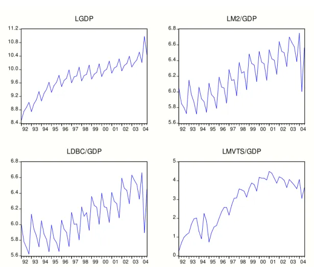
Figure 1 Time series

8.4 8.8 9.2 9.6 10.0 10.4 10.8 11.2 92 93 94 95 96 97 98 99 00 01 02 03 04 LGDP 5.6 5.8 6.0 6.2 6.4 6.6 6.8 92 93 94 95 96 97 98 99 00 01 02 03 04 LM2/GDP 5.6 5.8 6.0 6.2 6.4 6.6 6.8 92 93 94 95 96 97 98 99 00 01 02 03 04 LDBC/GDP 0 1 2 3 4 5 92 93 94 95 96 97 98 99 00 01 02 03 04 LMVTS/GDP

Figure 1 shows that three of the four series show a clear seasonal pattern. There are conflicting views about whether seasonally adjusted or unadjusted data should be used in this type of causality analysis. Here we follow Maddala and Kim (1998, p364) and do not prefilter the data as the initial step of our empirical analysis. Financial depth and domestic credit show a sharp decline in 2003.2. We treat this observation as genuine ones, and do not comment it out.4

The results of the ADF test for the existence of unit roots are reported in Table 1. We find that all our series can be treated as I(1) in the sample 1990.I–2004.III.

Table 1 Augmented Dickey-Fuller unit root test outcomes

trend constant # of lags ADF p-value LGDP level yes yes 5 -1.550 0.797

first differences no yes 3 -3.693 0.007 LM2/GDP level no No 3 2.718 0.998 first differences no yes 3 -17.235 0.000 LDBC/GDP level no yes 4 -0.973 0.755 first differences no No 3 -3.714 0.000 LMVTS/GDP level no yes 2 -1.908 0.326 first differences no No 1 -7.749 0.000

Note: critical values (5% level) of the ADF statistic are approximately equal to 3.51 (trend, constant),

-2.92 (no trend, constant) and -1.95 (no trend, no constant).

4

However, in order to test the sensitivity for this possible outlier, we also did all estimates without this observation, but this didn’t change the main results. For reasons of space, we have not presented these results. Of course, these estimates can be

5. Estimation Results

Given the limited number of observations to estimate our 4-variable VAR system, we set the maximum of lags to three and run lag exclusion tests. Table 2 shows the

results. All three lags enter the VAR system, so we proceed with a VAR of order three which corresponds to a VECM with two lags.

Table 2 Chi-squared statistics for lag exclusion tests (p-values between [])

LGDP LM2/GDP LDBC/GDP LMVTS/GDP Joint Lag 1 10.708 11.491 13.600 12.940 85.955 [ 0.030] [ 0.022] [ 0.009] [ 0.012] [ 1.38e-11] Lag 2 3.876 3.609 2.921 6.111 24.178 [ 0.423] [ 0.462] [ 0.571] [ 0.191] [ 0.086] Lag 3 7.509 5.949 4.240 14.749 41.011 [ 0.111] [ 0.203] [ 0.374] [ 0.005] [ 0.001] Df 4 4 4 4 16

The Johansen procedure tests for the form in which deterministic components enter the system and the number of cointegrating vectors. The constant and trend may enter the LR equations or the short run part of the VECM of Equation (2), leading to five possible outcomes.

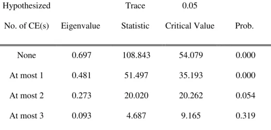
The best specification is to be decided on an information criterion. We apply the Schwarz criterion here, with an intercept in the long run and no trend. Johansen test outcomes for this trend assumption are listed in Table 3. We conclude that our VECM has two cointegrating vectors.

Table 3 Johansen test outcomes (restricted constant, no trend)

Hypothesized Trace 0.05

No. of CE(s) Eigenvalue Statistic Critical Value Prob.

None 0.697 108.843 54.079 0.000 At most 1 0.481 51.497 35.193 0.000 At most 2 0.273 20.020 20.262 0.054 At most 3 0.093 4.687 9.165 0.319

The cointegrating vectors normalized on economic growth and financial depth, respectively, are presented in the second and third columns of Table 4. The last two columns of this table list the two cointegrating vectors for which overidentification restrictions are taken into account. The Likelihood Ratio (LR) test for binding

restrictions indicates that exclusion of financial depth in the first cointegrating vector, exclusion of economic growth and and linear homogeneity between financial depth and banking sector development, and the two normalization restrictions not rejected by the data.

Cointegrating Eq: CointEq1 CointEq2 CointEq1 CointEq2

Normalized Normalized Overidentification Overidentification

LGDP-1 1.000 0.000 1.000 0.000 (LM2/GDP)-1 0.000 1.000 0.000 1.000 (LDBC/GDP)-1 -4.113 -1.135 -3.167 -1.000 (0.905) (0.117) (0.304) [-4.546] [-9.690] [-10.434] (LMVTS/GDP)-1 1.496 0.146 1.105 0.090 (0.263) (0.034) (0.114) (0.016) [ 5.679] [ 4.273] [ 7.662] [ 5.563] C 7.253 -0.155 3.357 -0.712 (4.798) (0.621) (1.733) (0.091) [ 1.512] [-0.249] [ 1.937] [-7.857]

LR test for binding restrictions (rank = 2): Chi-square(1)

Probability

0.403 0.526

Note: standard deviations between brackets, t-values between square brackets.

The long-run relationships for the normalized and the overidentified system show a similar picture. Here we base the interpretation on the overidentifed system. The first vector shows a positive relationship between financial depth and economic growth. It also indicates that stock market capitalization has a negative relationship with

level. The second vector displays a positive long-run relationship between financial depth and banking sector development, whereas stock market development is negatively associated with financial depth. Most importantly, the table suggests a positive long-run relationship between economic growth, financial depth and banking sector development. Surprisingly, there does not seem to be a positive long-run relationship between stock market development and economic growth.

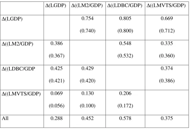
Finally, we consider short run causality and long-run weak exogeneity tests, both for the normalized and overidentified systems. Table 5 shows that there is no evidence of short-run causality in the system, except for a causal effect of stock market

development on economic growth (see first column). The latter, however, is only significant at the 10% significance level. This holds for the normalized and overidentified systems.

Table 5: Short-run Granger causality tests

∆(LGDP) ∆((LM2/GDP) ∆((LDBC/GDP) ∆((LMVTS/GDP) ∆(LGDP) 0.754 (0.740) 0.805 (0.800) 0.669 (0.712) ∆((LM2/GDP) 0.386 (0.367) 0.548 (0.532) 0.335 (0.360) ∆((LDBC/GDP 0.425 (0.421) 0.429 (0.420) 0.374 (0.386) ∆((LMVTS/GDP) 0.069 (0.056) 0.130 (0.100) 0.206 (0.172) All 0.288 0.452 0.578 0.375

(0.237) (0.386) (0.519) (0.382)

Note: the first row presents the dependent variables. The first column presents the excluded variables.

Figures are p-values for the chi-square statistic (low p-values indicate that the variable may not be

excluded). The p-values based on the over-identified system are given between brackets.

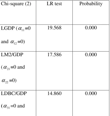
The results of the long-run causality, i.e. weak-exogeneity tests for the normalized system are given in Table 6. This table presents a joint test on both elements of alpha. Table 7 presents the results for the overidentified system. In this table, both elements of alpha are tested separately. Both tables lead to the same conclusions that the stock market variable is weakly exogenous to the system. Thus, the long-run relationships play no role in the equation for stock market development as adjustment does not take place. On the other hand, feedback relations exist between the other variables in the system and the two long cointegrating vectors.

Table 6: Weak exogeneity tests on normalized system. Chi-square (2) LR test Probability

LGDP (α₁₁=0 and α₁₂=0) 19.568 0.000 LM2/GDP (α₂₁=0 and 22 α =0) 17.586 0.000 LDBC/GDP (α₃₁=0 and 14.860 0.000

32 α =0) LMVTS/GDP (α₄₁=0 and 42 α =0) 2.288 0.319

Table 7: Weak-exogeneity tests on identified system

Hypothesis LR test Probability

11 α =0 _{18.391 0.000} 12 α =0 _{7.981 0.018} 21 α =0 _{17.291 0.000} 22 α =0 _{8.811 0.012} 31 α =0 _{14.638 0.001} 32 α =0 _{7.251 0.027} 41 α =0 _{1.131 0.568} 42 α =0 _{0.405 0.817} 6. CONCLUSIONS

This paper examines the relationship between economic growth, financial depth, banking sector development and stock market development for China. By utilizing cointegration techniques and testing for short-run noncausality and long-run weak exogeneity we find evidence for long-run positive relationships between financial depth, banking sector development and economic growth. The most striking result is

the effect of stock market development, which seems not to have contributed to long-run economic growth in China. Thus, our study provides support to authors such as Singh (1997) who questions the positive role of stock market development in the long-run. Singh (1997) argues that stock markets do not perform the monitoring, screening and disciplinary role very well, especially in emerging markets where the regulatory infrastructure is badly developed and stock markets are very thin, leading to excessive volatile share prices. Stock markets may also suffer from short-termism.

References

Allen, Franklin, Jun Qian and Meijun Qian (2002), Law, Finance, and Economic Growth in China, Working Paper Series of the Wharton Financial Institutions Center, 02-44.

Arestis, Philip, and Panicos Demetriades (1997), “Financial Development and Economic Growth: Assessing the Evidence,” Economic Journal, 107, 783-99.

Arestis, Philip, Panicos Demetriades and Kul B. Luintel (2001), “Financial

Development and Economic Growth: The Role of Stock Markets,”Journal of Money, Credit and Banking, 33, 16-41.

Arestis, Philip, Ambika D. Luintel and Kul B. Luintel (2004), Does Financial Structure Matter?, The Levy Economics Institute of Bard College, Working Paper No. 399.

Atje, R. and B. Jovanovic (1993), “Stock Markets and Development,” European Economic Review, 37, 632-40.

Barro, Robert J. (1991), “Economic Growth in a Cross Section of Countries,” Quarterly Journal of Economics, 105, 2, 407-43.

Unpublished.

Beck, T.A., Asli Demirguc-Kunt and Ross Levine (1999), A New Database on Financial Development and Structure, Policy Research Working Paper 2146, Washington: The World Bank.

Beck, T., Ross Levine and N. Loyaza (2000), “Finance and the Sources of Growth,” Journal of Financial Economics, 58, 261-300.

Bencivenga, Valerie R. and Bruce D. Smith (1991), “Financial Intermediation and Endogenous Growth,” Review of Economic Studies, 58, 195-209.

Bencivenga, Valerie R. and Bruce D. Smith (1993), “Some Consequences of Credit Rationing in an Endogenous Growth Model,” Journal of Economic Dynamics and Control, 17, 1-2, 97-122.

Berthelemy, Jean-Claude and Aristomene Varoudakis (1996), Financial Developemnt, Policy and Economic Growth, in Niels Hermes and Robert Lensink (eds), Financial Development and Economic Growth: Theory and Experiences from Developing Countries, London: Routledge, 66-94.

Christopoulos, Dimitris K. and Efthymios G. Tsionas (2004), “Financial Development and Economic Growth : Evidence from Panel Unit Root and Cointegration

Demetriades, P., and K. Hussein (1996), “Does Financial Development Cause Economic Growth? Time Series Evidence from 16 Countries,” Journal of Development Economics, 15, 387-411.

Engle, Robert F. and Clive W.J. Granger (1987, “Co-integration and Error Correction: Representation, Estimation, and Testing,” Econometrica, 55, 251-276.

Goldsmith, Raymond (1969), Financial Structure and Development, New Haven, CT: Yale University Press.

Green, S. (2003a), “China’s Stock Market: Eight Myths and Some Reasons to Be Optimistic,” Asia Programme Working Paper, Royal Institute of International Affairs.

Green, S. (2003b),

“

Greenwood, Jeremy and Boyan Jovanovic (1990), “Financial Development, Growth and the Distribution of Income,” Journal of Political Economy, 98, 5, 1076-107.

Gurley, John G. and Edward S. Shaw (1955), “Financial Aspects of Economic Development,” American Economic Review, 45, 4, 515-38.

Gurley, John G. and Edward S. Shaw (1960), Money in a Theory of Finance, Washington, DC: The Brookings Institution.

Johansen, Sören (1988), “Statistical Analysis of Cointegrating Vectors,” Journal of Economic Dynamics and Control, 12, 231-54.

Johansen, Sören (1991), Estimation and Hypothesis Testing of Cointegrating Vectors in Gaussian Vector Autoregressive Models,” Econometrica, 59, 551-80.

King, Robert G. and Ross Levine (1993a), “Finance, Entrepreneurship, and Growth: Theory and Evidence,” Journal of Monetary Economics, 32, 3, 513-42.

King, Robert G. and Ross Levine (1993b), “Finance and Growth: Schumpeter Might be Right,” Quarterly Journal of Economics, 108, 3, 717-37.

King, Robert G. and Ross Levine (1993c), “Financial Intermediation and Economic Growth,”in Colin Mayer and avier Vives (eds.), Capital Market and Financial Intermediation, Cambridge: Cambridge University Press, 156-89.

Laurenceson, James (2002), “The Impact of Stock Markets on China’s Economic Development: Some Preliminary Assessments,” ISSN 1033-4661.

Levine, Ross (1997), “Financial Development and Economic Growth: Views and Agenda,” Journal of Economic Literature, 35, 688-726.

Levine, Ross and Sarah Zervos (1998), “Stock Markets, Banks, and Economic Growth,”American Economic Review, 88, 537-58.

Levine, Ross, N. Loyaza and T. Beck (2000), “Financial Intermediation and Growth: Causality and Causes,” Journal of Monetary Economics, 46, 31-71.

Li, D.D. (2001), “Beating the Trap of Financial Repression in China,” Cato Journal 21.

Liu, L.G. (2002), “Sequencing Banking Sector Reforms in the People’s

Republic of China after the WTO: Options and Strategies Asian Development Bank”

Asian Development Bank working paper.

Maddala, G.S. and In-Moo Kim (1998), Unit Roots, Cointegration and Structural Change, Cambridge: Cambridge University Press.

Mehran, H. and M. Quintyn (1996), “Financial Sector Reforms in China.” Finance & Development.

Obstfeld, Maurice (1994), Risk-Taking, Global Diversification and Growth, American Economic Review, 84, 10-29.

Patrick, H.T. (1966), “Financial Development and Economic Growth in

Underdeveloped Countries,” Economic Development and Cultural Change, 14, 341-92.

Saint-Paul, Gilles (1992), “Technological Choice, Financial Markets and Economic Development,” European Economic Review, 36, 4, 763-81.

Saint-Paul, Gilles (1996), “Demand-driven Financial Development,”in Niels Hermes and Robert Lensink (eds), Financial Development and Economic Growth: Theory and Experiences from Developing Countries, London: Routledge, 37-52.

Schumpeter, Joseph A. (1939), Business Cycles: A Theoretical, Historical, and Statistical Analysis of the Capitalist Process, New York: McGraw-Hill.

Shirai, S. (2001), “Banking Sector Reforms in The People’s Republic of China-Progress and Constraints”, unpublished.

Shirai, S. (2002), “Is the Equity Market Really Developed in the People’s Republic of China?”ADB Institute Research paper 41.

Singh, A. (1997), “Financial Liberalization, Stock Markets and Economic Development,” The Economic Journal, 107, 771-82.

Toda, H.Y and P.C.B. Phillips (1993), “Vector Autoregressions and Causality,” Econometrica, 61, 1367-1393.

Toda, H.Y and P.C.B. Phillips (1994), “Vector Autoregression and Causality: A Theoretical Overview and Simulation Study,” Econometric Reviews, 13, 259-285.

Xiang, B. (1998), “The Reform of China’s Large State-Owned Enterprises: The Indispensable Role of Stock Markets,” in J. Cheng (ed.), China in the Post-Deng Era, Hong Kong: The Chinese University Press, pp. 311-328.

Data Sources

Annual data: 1. M2 :

1978-2002 are from each year’s Almanac of China’ Finance and Banking, 2003 is from the website of The People’s Bank of China.

2. GDP :

1978-2002 are from each year’s Statistical Yearbook of China. 2003 is from the website of Chinese National Statistical Bureau. 3. Domestic bank credit and Total assets of domestic banks

1993-1999 are from The People’s Bank of China Quarterly Statistical Bulletin. 2000-2003 are from the website of The People’s Bank of China, because there was 4.National bank credit :

1978-1992, are from Almanac of China’ Finance and Banking 4.Listed Companies, Market Capitalization and Total Raised Capital :

1992 -1998 is from Almanac of China’ Finance and Banking ,

1999 –2003 is from the website of China Securities Regularity Committee.

Quartarly data: 1.GDP:

1992.Q1-2000.Q4 are from Chinese National Statistical Bureau.

2001.Q1-2004.Q3 are from the website of Chinese National Statistical Bureau. 2.M2:

1992.Q1-2003.Q4 are from The People’s Bank of China Quarterly Statistical Bulletin, 2004.Q1-2004.Q3 is from the website of The People’s Bank of China.

3. Domestic bank credit :

1993.Q1-1999.Q4 are from The People’s Bank of China Quarterly Statistical Bulletin, 2000.Q1-2004.Q3 are from the website of The People’s Bank of China. Because the 4.Commercial bank credit :

1992.Q1-1992.Q4 are from the website of IFM (http://ifs.apdi.net/imf/logon.aspx). 5.Market value of tradable stock:

1995.Q1-1998.Q4 are from The People’s Bank of China Quarterly Statistical Bulletin (1997, 1999),

1999.Q1-2004Q3 are from the website of China Securities Regularity Committee, the 1994 Q1-1994Q4 are from the website of IFM (http://ifs.apdi.net/imf/logon.aspx), 1992 Q1-1993.Q4 are estimated according to the yearly data. The yearly data is from Almanac of China’ Finance and Banking