3. VERILOG HARDWARE DESCRIPTION LANGUAGE

(1)

3.

VERILOG HARDWARE

DESCRIPTION

LANGUAGE

The previous chapter describes how a designer may manually use ASM charts (to scribe behavior) and block diagrams (to describe structure) in top-down hardware de-sign. The previous chapter also describes how a designer may think hierarchically, where one module’s internal structure is defined in terms of the instantiation of other modules. This chapter explains how a designer can express all of these ideas in a spe-cial hardware description language known as Verilog. It also explains how Verilog can test whether the design meets certain specifications.

3.1

Simulation versus synthesis

Although the techniques given in chapter 2 work wonderfully to design small machines by hand, for larger designs it is desirable to automate much of this process. To automate hardware design requires a Hardware Description Language (HDL), a different nota-tion than what we used in chapter 2 which is suitable for processing on a general-purpose computer. There are two major kinds of HDL processing that can occur: simu-lation and synthesis.

Simulation is the interpretation of the HDL statements for the purpose of producing human readable output, such as a timing diagram, that predicts approximately how the hardware will behave before it is actually fabricated. As such, HDL simulation is quite similar to running a program in a conventional high-level language, such as Java Script, LISP or BASIC, that is interpreted. Simulation is useful to a designer because it allows detection of functional errors in a design without having to fabricate the actual hard-ware. When a designer catches an error with simulation, the error can be corrected with a few keystrokes. If the error is not caught until the hardware is fabricated, correcting the problem is much more costly and complicated.

Synthesis is the compilation of high-level behavioral and structural HDL statements into a flattened gate-level netlist, which then can be used directly either to lay out a printed circuit board, to fabricate a custom integrated circuit or to program a program-mable logic device (such as a ROM, PLA, PLD, FPGA, CPLD, etc.). As such, synthe-sis is quite similar to compiling a program in a conventional high-level language, such as C. The difference is that, instead of producing object code that runs on the same computer, synthesis produces a physical piece of hardware that implements the compu-tation described by the HDL code. For the designer, producing the netlist is a simple

(2)

step (typically done with only a few keystrokes), but turning the netlist into physical hardware is often costly, especially when the goal is to obtain a custom integrated circuit from a commercial silicon foundry. Typically after synthesis, but before the physical fabrication, the designer simulates the synthesized netlist to see if its behavior matches the original HDL description. Such post-synthesis simulation can prevent costly errors.

3.2

Verilog versus VHDL

HDLs are textual, rather than graphic, ways to describe the various stages in the top-down design process. In the same language, HDLs allow the designer to express both the behavioral and structural aspects of each stage in the design. The behavioral fea-tures of HDLs are quite similar to conventional high-level languages. The feafea-tures that make an HDL unique are those structural constructs that allow description of the instantiation and interconnection of modules.

There are many proprietary HDLs in use today, but there are only two standardized and widely used HDLs: Verilog and VHDL. Verilog began as a proprietary HDL promoted by a company called Cadence Data Systems, Inc., but Cadence transferred control of Verilog to a consortium of companies and universities known as Open Verilog Interna-tional (OVI). Many companies now produce tools that work with standard Verilog. Verilog is easy to learn. It has a syntax reminiscent of C (with some Pascal syntax thrown in for flavor). About half of commercial HDL work in the U.S. is done in Verilog. If you want to work as a digital hardware designer, it is important to know Verilog. VHDL is a Department of Defense (DOD) mandated language that is used primarily by defense contractors. Although most of the concepts in VHDL are not different from those in Verilog, VHDL is much harder to learn. It has a rigid and unforgiving syntax strongly influenced by Ada (which is an unpopular conventional programming lan-guage that the DOD mandated defense software contractors to use for many years be-fore VHDL was developed). Although more academic papers are published about VHDL than Verilog, less than one-half of commercial HDL work in the U.S. is done in VHDL. VHDL is more popular in Europe than it is in the U.S.

3.3

Role of test code

The original purpose of Verilog (and VHDL) was to provide designers a unified lan-guage for simulating gate-level netlists. Therefore, Verilog combines a structural nota-tion for describing netlists with a behavioral notanota-tion for saying how to test such netlists during simulation. The behavioral notation in Verilog looks very much like normal executable statements in a procedural programming language, such as Pascal or C. The original reason for using such statements in Verilog code was to provide stimulus to the

(3)

netlist, and to test the subsequent response of the netlist. The pairs of stimulus and response are known as test vectors. The Verilgo that creates the stimulus and observes the response is known as the test code or testbench. Snoopy's "woof" in the comic strip of section 2.2 is analougus to the role of the test codes warning us that the expected response was not observed. For example, one way to use simulation to test whether a small machine works is to do an exhaustive test, where the test code provides each possible combination of inputs to the netlist and then checks the response of the netlist to see if it is appropriate.

For example, consider the division machine of the last chapter. Assume we have devel-oped a flattened netlist that implements the complete machine. It would not be at all obvious whether this netlist is correct. Since the bus width specified in this problem is small (twelve bits), we can write Verilog test code using procedural Verilog (similar to statements in C) that does an exhaustive test. A reasonable approach would be to use two nested loops, one that varies x through all its 4096 possible values, and one that varies y through all its 4095 possible values. At appropriate times inside the inner loop, the test code would check (using an if statement) whether the output of the netlist matches x/y. Verilog provides most of the integer and logical operations found in C, including those, such as division, that are difficult to implement in hardware. The origi-nal intent was not to synthesize such code into hardware but to document how the netlist should automatically be tested during simulation.

Verilog has all of the features you need to write conventional high-level language pro-grams. Except for file Input/Output (I/O), any program that you could write in a con-ventional high- level language can also be written in Verilog. The original reason Verilog provides all this software power in a “hardware” language is because it is impossible to do an exhaustive test of a complex netlist. The 12-bit division machine can be tested exhaustively because there are only 16,773,120 combinations with the 24 bits of input to the netlist. A well-optimized version of Verilog might be able to conduct such a simulation in a few days or weeks. If the bus width were increased, say to 32-bits, the time to simulate all 264_{combinations would be millions of years. Rather than give up} on testing, designers write more clever test code. The test code will appear longer, but will execute in much less time. Of course, if a machine has a flaw that expresses itself for only a few of the 264_{test patterns, the probability that our fast test code will find the} flaw is usually low.

3.4

Behavioral features of Verilog

Verilog is composed of modules (which play an important role in the structural aspects of the language, as will be described in section 3.10). All the definitions and declara-tions in Verilog occur inside a module.

(4)

3.4.1

Variable declaration

At the start of a module, one may declare variables to be integer or to be real. Such variables act just like the software declarations int and float in C. Here is an example of the syntax:

integer x,y; real Rain_fall;

Underbars are permitted in Verilog identifiers. Verilog is case sensitive, and so

Rain_fall and rain_fall are distinct variables. The declarations integer and

real are intended only for use in test code. Verilog provides other data types, such as

reg and wire, used in the actual description of hardware. The difference between these two hardware-oriented declarations primarily has to do with whether the variable is given its value by behavioral (reg) or structural (wire) Verilog code. Both of these declarations are treated like unsigned in C. By default, regs and wires are only one bit wide. To specify a wider reg or wire, the left and right bit positions are defined in square brackets, separated by a colon. For example:

reg [3:0] nibble,four_bits;

declares two variables, each of which can contain numbers between 0 and 15. The most significant bit of nibble is declared to be nibble[3], and the least significant bit is declared to be nibble[0]. This approach is known as little endian notation. Verilog also supports the opposite approach, known as big endian notation:

reg [0:3] big_end_nibble;

where now big_end_nibble[3] is the least significant bit.

If you store a signed value1_{in a}_reg_{, the bits are treated as though they are unsigned.} For example, the following:

four_bits = -5;

is the same as:

four_bits = 11;

1 _{In order to simplify dealing with twos complement values, many implementations allow integers with an} arbitrary width. Such declarations are like regs, except they are signed.

(5)

Verilog supports concatenation of bits to form a wider wire or reg, for example,

{nibble[2], nibble[1]} is a two bit reg composed of the middle two bits of

nibble. Verilog also provides a shorthand for obtaining a contiguous set of bits taken from a single reg or wire. For example, the middle two bits of nibble can also be specified as nibble[2:1]. It is legal to assign values using either of these notations. Verilog also allows arrays to be defined. For example, an array of reals could be defined as:

real monthly_precip[11:0];

Each of the twelve elements of the array (from monthly_precip[0] to

monthly_precip[11]) is a unique real number. Verilog also allows arrays of wires and regs to be defined. For example,

reg [3:0] reg_arr[999:0]; wire[3:0] wir_arr[999:0];

Here, reg_arr[0] is a four-bit variable that can be assigned any number between 0 and 15 by behavioral code, but wir_arr[0] is a four-bit value that cannot be as-signed its value from behavioral code. There are one thousand elements, each four bits wide, in each of these two arrays. Although the [] means bit select for scalar values, such as nibble[3], the [] means element select with arrays. It is illegal to com-bine these two uses of [] into one, as in if(reg_arr[0][3]). To accomplish this operation requires two statements:

nibble = reg_arr[0]; if (nibble[3]) ...

3.4.2

Statements legal in behavioral Verilog

The behavioral statements of Verilog include2_{the following:}

var = expression;

if (condition) statement

2 _{There are other, more advanced statements that are legal. Some of these are described in chapters 6} and 7.

(6)

if (condition) statement else statement while (condition) statement for (var=expression;condition;var=var+expression) statement forever statement case (expression) constant: statement ... default: statement endcase

where the italic statement, var, expression, condition and constant are replaced with appropriate Verilog syntax for those parts of the language. A state-ment is one of the above statements or a series of the above statements terminated by semicolons inside begin and end. A var is a variable declared as integer, real, reg or a concatenation of regs. A var cannot be declared as wire.

3.4.3

Expressions

An expression involves constants and variables (including wires) with arithmetic (+ , - , * , / , %), logical (& , & & , | , | | , ^ , ~ , < < , > >), relational (<,==,===,<=,>=,!=,!==,>) and conditional (?:) operators. A condition

is an expression. A condition might be an expression involving a single bit, (as would be produced by ||, &&, !, <, ==, ===, <=, >=, !=, !== or >) or an expression involving several bits that is checked by Verilog to see if it is equal to 1. Except for === and !==, these symbols have the same meaning as in C. Assuming the result is stored in a 16-bit reg,3_{the following table illustrates the result of these}

operators, for example where the left operand (if present) is ten and the right operand is three:

Continued

(7)

symbol name example 16-bit unsigned result + addition 10+3 13 - subtraction 10-3 7 - negation -10 65526 * multiplication 10*3 30 / division 10/3 3 % remainder 10%3 1 << shift left 10<<3 80 >> shift right 10>>3 1

& bitwise AND 10&3 2

| bitwise OR 10|3 11 ^ bitwise exclusive OR 10^3 9 ~ bitwise NOT ~10 65525 ?: conditional operator 0?10:3 3 1?10:3 10 ! logical NOT !10 0

&& logical AND 10&&3 1

|| logical OR 10||3 1

< less than 10<3 0

== equal to 10==30

<= less than or equal to 10<=3 0 >= greater than or equal 10>=3 1

!= not equal 10!=3 1

> greater than 10>3 1

3.4.4

Blocks

All procedural statements occur in what are called blocks that are defined inside mod-ules, after the type declarations. There are two kinds of procedural blocks: the

initial block and the always block. For the moment, let us consider only the

initial block. An initial block is like conventional software. It starts execution and eventually (assuming there is not an infinite loop inside the initial block) it stops execution. The simplest form for a single Verilog initial block is:

(8)

module top; declarations; initial begin statement; ... statement; end endmodule

The name of the module (t o p in this case) is arbitrary. The syntax of the

declarations is as described above. All variables should be declared. Each state-ment is terminated with a semicolon. Verilog uses the Pascal-like begin and end,

rather than { and }. There is no semicolon after begin or end. The begin and end

may be omitted in the rare case that only one procedural statement occurs in the ini-tial block.

Here is an example that prints out all 16,773,120 combinations of values described in section 3.3: module top; integer x,y; initial begin x = 0; while (x<=4095) begin

for (y=1; y<=4095; y = y+1) begin $display("x=%d y=%d",x,y); end x = x + 1; end end $write("all "); $display("done"); endmodule

The loop involving x could have been written as a for loop also but was shown above as a while for illustration. Note that Verilog does not have the ++ found in C, and so it is necessary to say something like y = y + 1. This assignment statement is just like

(9)

its counterpart in C: it is instantaneous. The variable changes value before the next statement executes (unlike the RTN discussed in the previous chapter). The $dis-play is a system task (which begin with $) that does something similar to what

printf("%d %d \n",x,y) does in C: it formats the textual output according to the string in the quotes. The system task $write does the same thing as $display, except that it does not produce a new line:

x= 0 y= 1 x= 0 y= 2 ... ... x= 4095 y= 4094 x= 4095 y= 4095 all done

The above code would fail if the declaration had been:

reg [11:0] x,y;

because, although twelve bits are adequate for the hardware, the test code requires that

x and y become 4096 in order for the loop to stop.

Since infinite loops are useful in hardware, Verilog provides the syntax forever, which means the same thing as while(1). In addition, the always block mentioned above can be described as an initial block containing only a forever loop. For simulation purposes, the following mean the same:

initial initial begin begin

while(1) forever always begin begin begin ... ... ... end end end end end

For synthesis, one should use the always block form only. The statement forever

is not a block and cannot stand by itself. Like other procedural statements, forever

(10)

3.4.5

Constants

By default, constants in Verilog are assumed to be decimal integers. They may be speci-fied explicitly in binary, octal, decimal, or hexadecimal by prefacing them with the syntax ’b,’o,’d, or ’h, respectively. For example, ’b1101,’o15,’d13, ’hd, and 13 all mean the same thing. If you wish to specify the number of bits in the representation, this proceeds the quote: 4’b1101,4’o15,4’d13,4’hd.

3.4.6

Macros,

include

files and comments

As an aid to readability of the code, Verilog provides a way to define macros. For example, the aluctrl codes described in 2.3.1 can be defined with:

‘define DIFFERENCE 6’b011001 ‘define PASSB 6’b101010

Later in the code, a reference to these macros (preceded by a backquote) is the same as substituting the associated value. The following ifs mean the same:

if (aluctrl == ‘DIFFERENCE) if (aluctrl == 6’b011001) $display("subtracting"); $display("subtracting");

Note the syntax difference between variables (such as aluctrl), macros (such as

‘DIFFERENCE), and constants (such as 6’b011001). Variables are not preceded by anything. Macros are preceded by backquote. Constants may include one forward single quote.

You can determine whether a macro is defined using ‘ifdef and ‘endif. This preprocessing feature should not be confused with if. For example, the following:

‘ifdef DIFFERENCE $display("defined"); ‘endif

prints the message regardless of the value of ‘DIFFERENCE, as long as that macro is defined. The message is not printed only when there is not a ‘ d e f i n e for

‘DIFFERENCE.

Verilog allows you to separate your source code into more than one file (just like #in-clude in C and {$I} in Pascal). To use code contained in another file, you say:

(11)

There are two forms of comments in Verilog, which are the same as the two forms found in C++. A comment that extends only for the rest of the current line can occur after //. A comment that extends for several lines begins with /* and ends with */. For example:

/* a multi line comment

that includes a declaration: reg a;

which is ignored by Verilog */

reg b; // this declaration is not ignored

3.5

Structural features of Verilog

Verilog provides a rich set of built-in logic gates, including and,or,xor,nand, nor,not and buf, that are used to describe a netlist. The syntax for these structural features of Verilog is quite different than for any of the behavioral features of Verilog mentioned earlier. The outputs of such gates are declared to be wire, which by itself describes a one-bit data type. (Regardless of width, an output generated by structural Verilog code must be declared as a wire.) The inputs to such gates may be either declared as wire or reg (depending on whether the inputs are themselves computed by structural or behavioral code). To instantiate such a gate, you say what kind of gate you want (xor for example) and the name of this particular instance (since there may be several instances of xor gates, let’s name this example x1). Following the instance name, inside parentheses are the output and input ports of the gate (for example, say the output is a wire named c, and the inputs are a and b). The output(s) of gates are always on the left inside the parentheses:

module easy_xor; reg a,b; wire c; xor x1(c,a,b); ... endmodule

People familiar with procedural programming languages, like C, mistakenly assume this is “passing c, a and b and then calling on xor.” It is doing no such thing. It simply says that an xor gate named x1 has its output connected to c and its inputs connected to a and b. If you are familiar with graph theory, this notation is simply a way to describe the edges (a,b,c) and vertex (x1) of a graph that represents the structure of a circuit.

(12)

3.5.1

Instantiating multiple gates

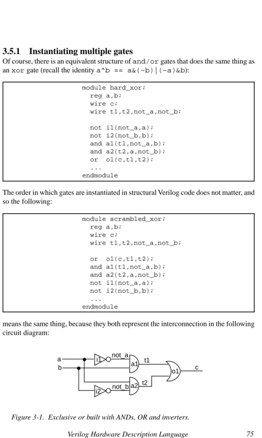
Of course, there is an equivalent structure of and/or gates that does the same thing as an xor gate (recall the identity a^b == a&(~b)|(~a)&b):

module hard_xor; reg a,b; wire c; wire t1,t2,not_a,not_b; not i1(not_a,a); not i2(not_b,b); and a1(t1,not_a,b); and a2(t2,a,not_b); or o1(c,t1,t2); ... endmodule

The order in which gates are instantiated in structural Verilog code does not matter, and so the following: module scrambled_xor; reg a,b; wire c; wire t1,t2,not_a,not_b; or o1(c,t1,t2); and a1(t1,not_a,b); and a2(t2,a,not_b); not i1(not_a,a); not i2(not_b,b); ... endmodule

means the same thing, because they both represent the interconnection in the following circuit diagram:

Figure 3-1. Exclusive or built with ANDs, OR and inverters.

a i1 i2 b not_a not_b t1 t2 c a1 a2 o1

(13)

3.5.2

Comparison with behavioral code

Structural Verilog code does not describe the order in which computations implemented by such a structure are carried out by the Verilog simulator. This is in sharp contrast to behavioral Verilog code, such as the following:

module behavioral_xor; reg a,b; reg c; reg t1,t2,not_a,not_b; always ... begin not_a = ~a; not_b = ~b; t1 = not_a&b; t2 = a&not_b; c = t1|t2; end endmodule

which is a correct behavioral rendition of the same idea. (The ellipses must be replaced by a Verilog feature described later.) Also, c, t1, t2, not_a and not_b must be declared as regs because this behavioral (rather than structural) code assigns val-ues to them.

To rearrange the order of behavioral assignment statements is incorrect:

module bad_xor; reg a,b; reg c; reg t1,t2,not_a,not_b; always ... begin c = t1|t2; t1 = not_a&b; t2 = a&not_b; not_a = ~a; not_b = ~b; end endmodule

(14)

3.5.3

Interconnection errors: four-valued logic

In software, a bit is either a 0 or a 1. In properly functioning hardware, this is usually the case also, but it is possible for gates to be wired together incorrectly in ways that produce electronic signals that are neither 0 nor 1. To more accurately model such physical possibilities,4_{each bit in Verilog can be one of four things:}_{1’b0, 1’b1,} 1’bz or 1’bx.

Obviously, 1’b0 and 1’b1 correspond to the logical 0 and logical 1 that we would normally expect to find in a computer. For most technologies, these two possibilities are represented by a voltage on a wire. For example, active high TTL logic would represent 1’b0 as zero volts and 1’b1 as five volts. Active low TTL logic would represent 1’b0 as five volts and 1’b1 as zero volts. Other kinds of logic families, such as CMOS, use different voltages. ECL logic uses current, rather than voltage, to represent information, but the concept is the same.

3.5.3.1

High impedance

In any technology, it is possible for gates to be miswired. One kind of problem is when a designer forgets to connect a wire or forgets to instantiate a necessary gate. This means that there is a wire in the system which is not connected to anything. We refer to this as high impedance, which in Verilog notation is 1’bz. The TTL logic family will normally view high impedance as being the same as five volts. If the input of a gate to which this wire is connected is active high, 1’bz will be treated as 1’b1, but if it is active low, it will be treated as 1’b0. Other logic families treat 1’bz differently. Fur-thermore, electrical noise may cause 1’bz to be treated spuriously in any logic family. For these reasons, it is important for a Verilog simulator to treat 1’bz as distinct from

1’b0 and 1’b1. For example, if the designer forgets the final or gate in the example from section 3.5.1: module forget_or_that_outputs_c; reg a,b; wire c; wire t1,t2,not_a,not_b; not i1(not_a,a); not i2(not_b,b); and a1(t1,not_a,b); and a2(t2,a,not_b); ... endmodule

4 _{Verilog also allows each bit to have a strength, which is an electronic concept (below gate level) beyond the} scope of this book.

(15)

there is no gate that outputs the wire c, and therefore it remains 1’bz, regardless of what a and b are.

3.5.3.2

Unknown value

Another way in which gates can be miswired is when the output of two gates are wired together. This raises the possibility of fighting outputs, where one of the gates wants to output a 1’b0, but the other wants to output a 1’b1. For example, if we tried to eliminate the or gate by tying the output of both and gates together:

module tie_ands_together; reg a,b; wire c; wire t1,t2,not_a,not_b; not i1(not_a,a); not i2(not_b,b); and a1(c,not_a,b); and a2(c,a,not_b); ... endmodule

the result is correct (1’b0) when a and b are the same because the two and gates both produce 1’b0 and there is no fight. The result is incorrect (1’bx) when a is 1’b0 and

b is 1’b1 or vice versa, because the two and gates fight each other. Fighting gates can cause physical damage to certain families of logic (i.e., smoke comes out of the chip). Obviously, we want to be able to have the simulator catch such problems before we fabricate a chip that is doomed to blow up (literally)!

3.5.3.3

Use in behavioral code

Behavioral code may manipulate bits with the four-valued logic. Uninitialized regs in behavioral code start with a value of ’bx. (As mentioned above for structural code, disconnected wires start with a value of ’bz.) All the Boolean operators, such as &, | and ~ are defined with the four-valued logic so that the usual rules of commutativity, associativity, etc. apply.

The four-valued logic may be used with multi-bit wires and regs. When all the bits are either 1’b1 or 1’b0, such as 3’b110, the usual binary interpretation (powers of two) applies. When any of the bits is either 1’bz or 1’bx, such as 3’b1z0, the numeric value is unknown.

(16)

Arithmetic and relational operators (including == and !=) produce their usual results only when both operands are composed of 1’b0s and 1’b1s. In any other case, the result is ’bx. This relates to the fact the corresponding combinational logic required to implement such operations in hardware would not produce a reliable result under such circumstances. For example:

if ( a == 1’bx)

$display("a is unknown");

will never display the message, even when a is 1’bx, because the result of the ==

operation is always 1’bx. 1’bx is not the same as 1’b1, and so the $display

never executes.

There are two special comparison operators (=== and !==) that overcome this limita-tion. === and !== cannot be implemented in hardware, but they are useful in writing intelligent simulations. For example:

if ( a === 1’bx)

$display("a is unknown");

will display the message if and only if a is 1’bx.

To help understand the last examples, you should realize that the following two if

statements are equivalent:

if(expression) if((expression)===1’b1) statement; statement;

The following table summarizes how the four-valued logic works with common opera-tors:

(17)

This table was generated by the following Verilog code: module xz01; reg a,b,val[3:0]; integer ia,ib; initial begin val[0] = 1’b0; val[1] = 1’b1; val[2] = 1’bx; val[3] = 1’bz; $display

("a b a==b a===b a!=b a!==b a&b a&&b a|b a||b a^b");

for (ia = 0; ia<=3; ia=ia+1) for (ib = 0; ib<=3; ib=ib+1) begin a = val[ia]; b = val[ib]; $display ("%b %b %b %b %b %b %b %b %b %b %b ", a,b,a==b,a===b,a!=b,a!==b,a&b,a&&b,a|b,a||b,a^b); end end endmodule

a b a==b a===b a!=b a!==b a&b a&&b a|b a||b a^b

0 0 1 1 0 0 0 0 0 0 0 0 1 0 0 1 1 0 0 1 1 1 0 x x 0 x 1 0 0 x x x 0 z x 0 x 1 0 0 x x x 1 0 0 0 1 1 0 0 1 1 1 1 1 1 1 0 0 1 1 1 1 0 1 x x 0 x 1 x x 1 1 x 1 z x 0 x 1 x x 1 1 x x 0 x 0 x 1 0 0 x x x x 1 x 0 x 1 x x 1 1 x x x x 1 x 0 x x x x x x z x 0 x 1 x x x x x z 0 x 0 x 1 0 0 x x x z 1 x 0 x 1 x x 1 1 x z x x 0 x 1 x x x x x z z x 1 x 0 x x x x x

(18)

3.6

$time

A Verilog simulator executes as a software program on a conventional general-purpose computer. How long it takes such a computer to run a Verilog simulation, known as real time, depends on several factors, such as how fast the general-purpose computer is, and how efficient the simulator is. The speed with which the designer obtains the simula-tion results has little to do with how fast the eventual hardware will be when it is fabri-cated. Therefore, the real time required for simulation is not important in the following discussion.

Instead, Verilog provides a built-in variable, $time, which represents simulated time, that is, a simulation of the actual time required for a machine to operate when it is fabricated. Although the value of $time in simulation has a direct relationship to the physical time in the fabricated hardware, $time is not measured in seconds. Rather,

$time is a unitless integer. Often designers map one of these units into one nanosec-ond, but this is arbitrary.

3.6.1

Multiple blocks

Verilog allows more than one behavioral block in a module. For example:

module two_blocks; integer x,y; initial begin a=1; $display("a is one"); end initial begin b=2; $display("b is two"); end endmodule

The above simulates a system in which a and b are simultaneously assigned their respective values. This means, from a simulation standpoint, $time is the same when

a is assigned one as when b is assigned two. (Since both assignments occur in ini-tial blocks, $time is 0.) Note that this does not imply the sequence in which these assignments (or the corresponding $display statements) occur.

(19)

3.6.2

Sequence versus

$time

In software, we often confuse the two separate concepts of time and sequence. In Verilog, it is possible for many statements to execute without $time advancing. The sequence in which statements within one block execute is determined by the usual rules found in other high-level languages. The sequence in which statements within different blocks execute is something the designer cannot predict, but that Verilog will do consistently. The advancing of $time is a different issue, discussed in section 3.7.

If you change the wires to be regs, a structural Verilog netlist is equivalent to several

always blocks, where each always block computes the result output by one gate. If the design is correct, the sequence in which such always blocks execute at a particu-lar $time is irrelevant, which helps explain why the order in which you instantiate gates in structural Verilog is also irrelevant. With Verilog, you can simulate the parallel actions of each gate or module that you instantiate, as well as the parallel actions of each behavioral block you code.

3.6.3

Scheduling processes and deadlock

Like a multiprocessing operating system, a Verilog simulator schedules several pro-cesses, one for each structural component or behavioral block. The $time variable does not advance until the simulator has given each process that so desires an opportu-nity to execute at that $time.

If you are familiar with operating systems concepts, such as semaphores, you will recognize that this raises a question about how Verilog operates: what are the atomic units of computation, or in other words, when does a process get interrupted by the Verilog simulator?

The behavioral statements described earlier are uninterruptible. Although it is nearly correct to model an exclusive OR with the following behavioral code:

module deadlock_the_simulator; reg a,b,c; always c = a^b; ... other blocks ... endmodule

the Verilog simulator would never allow the other blocks to execute because the block computing c is not interruptible. Overcoming this problem requires an additional fea-ture of Verilog, discussed in the next section.

(20)

3.7

Time control

Behavioral Verilog may include time control statements, whose purpose is to release control back to the Verilog scheduler so that other processes may execute and also tell the Verilog simulator at what $time the current process would like to be restarted. There are three forms of time control that have different ways of telling the simulator when to restart the current process: #, @ and wait.

3.7.1

# time control

When a statement is preceded by # followed by a number, the scheduler will not ex-ecute the statement until the specified number of $time units have passed. Any other process that desires to execute earlier than the $time specified by the # will execute before the current process resumes. If we modify the first example from section 3.6:

module two_blocks_time_control; integer x,y; initial begin #4 a=1;

$display("a is one at $time=%d",$time); end

initial begin #3 b=2;

$display("b is two at $time=%d",$time); end

endmodule

the above will assign first to b (at $time=3) and then to a one unit of $time later. The order in which these statements execute is unambiguous because the # places them at a certain point in $time.

There can be more than one # in a block. The following nonsense module illustrates how the # works:

(21)

In the above code, a becomes 10 at $time 0, 40 at $time 1, 20 at $time 2, 50 at

$time 4, 30 at $time 7 and 60 at $time 8. The interaction of parallel blocks creates a behavior much more complex than that of each individual block.

3.7.1.1 Using # in test code

One of the most important uses of # is to generate sequences of patterns at specific

$times in test code to act as inputs to a machine. The # releases control from the test code and gives the code that simulates the machine an opportunity to execute. Test code without some kind of time control would be pointless because the machine being tested would never execute.

For example, suppose we would like to test the built-in xor gate by stimulating it with all four combinations on its inputs, and printing the observed truth table:

module confusing; integer a; initial begin a = 10; #2 a = 20; #5 a = 30; end initial begin #1 a = 40; #3 a = 50; #4 a = 60; end endmodule

(22)

The first time through, a and b are initialized to be 0 at $time 0. When #10 executes at $time 0, the initial block relinquishes control, and x1 is given the opportunity to compute a new value (0^0=0) on the wire c. Having completed everything sched-uled at $time 0, the simulator advances $time. The next thing scheduled to execute is the $display statement at $time 10. (The simulator does not waste real time computing anything for $time 2 through 9 since nothing changes during this $time.) The simulator prints out that “a=0 b=0 c=0” at $time 10 and then goes through the inner loop once again. While $time is still 10, b becomes 1. The #10 relinquishes control, x1 computes that c is now 1 and $time advances. The $display prints out that “a=0 b=1 c=1” at $time 20. The last two lines of the truth table are printed out in a similar fashion at $times 30 and 40.

3.7.1.2

Modeling combinational logic with #

Physical combinational logic devices, such as the exclusive OR gate, have propagation delay. This means that a change in the input does not instantaneously get reflected in the output as shown above, but instead it takes some amount of physical time for the change to propagate through the gate. Propagation delay is a low-level detail of hard-ware design that ultimately determines the speed of a system. Normally, we will want to ignore propagation delay, but for a moment, let’s consider how it can be modeled in behavioral Verilog with the #.

module top; integer ia,ib; reg a,b; wire c; xor x1(c,a,b); initial begin

for (ia=0; ia<=1; ia = ia+1) begin

a = ia;

for (ib=0; ib<=1; ib = ib + 1) begin b = ib; #10 $display("a=%d b=%d c=%d",a,b,c); end end end endmodule

(23)

The behavioral exclusive OR example in section 3.6.3 deadlocks the simulator because it does not have any time control. If we put some time control in this always block (say a propagation delay of #1), the simulator will have an opportunity to schedule the test code instead of deadlocking inside the always block:

module top; integer ia,ib; reg a,b; reg c; always #1 c = a^b; initial begin

a = ia;

for (ib=0; ib<=1; ib = ib + 1) begin b = ib; #10 $display("a=%d b=%d c=%d",a,b,c); end end $finish; end endmodule

As in the last example, a and b are initialized to be 0 at $time 0. When #10 executes at $time 0, the initial block relinquishes control, which gives the always loop an opportunity to execute. The first thing that the always block does is to execute #1, which relinquishes control until $time 1. Since no other block wants to execute at

$time 1, execution of the always block resumes at $time 1, and it computes a new value (0^0=0) for the reg c. Because this is an always block, it loops back to the #1. Since no other block wants to execute at $time 2, execution of the always block resumes at $time 2, and it recomputes the same value for the reg c that it just com-puted at $time 1. The always block continues to waste real time by unnecessarily recomputing the same value all the way up to $time 9.

Finally, the $display statement executes at $time 10. The test code prints out “a=0 b=0 c=0” and goes through its inner loop once again. While $time is still 10, b

becomes 1. The #10 relinquishes control, and the always block will have another ten chances to compute that c is now 1. The remaining lines of the truth table are printed out in a similar fashion.

(24)

There is an equivalent structural netlist notation for an always block with # time control. The following behavioral and structural code do similar things in $time:

reg c; wire c;

always #2 xor #2 x2(c,a,b); c = a^b;

Both model an exclusive OR gate with a propagation delay of two units of $time. On many (but not all) implementations of Verilog simulators, the structural version is more efficient from a real-time standpoint. This is discussed in greater detail in chapter 6.

3.7.1.3

Generating the system clock with # for simulation

Registers and controllers are driven by some kind of a clock signal. One way to gener-ate such a signal is to have an initial block give the clock signal an initial value, and an always block that toggles the clock back and forth:

reg sysclk;

initial

sysclk = 0;

always #50

sysclk = ~sysclk;

The above generates a system clock signal, sysclk, with a period of 100 units of

$time.

3.7.1.4

Ordering processes without advancing

$time

It is permissible to use a delay of #0. This causes the current process to relinquish control to other processes that need to execute at the current $time. After the other processes have relinquished control, but before $time advances, the current process will resume. This kind of time control can be used to enforce an order on processes whose execution would otherwise be unpredictable. For example, the following is algorithmically the same as the first example in 3.7.1 (b is assigned first, then a), but both assignments occur at $time 0:

(25)

3.7.2

@ time control

When an @ precedes a statement, the scheduler will not execute the statement that follows until the event described by the @ occurs. There are several different kinds of events that can be specified after the @, as shown below:

@(expression)

@(expression or expression or ...) @(posedge onebit)

@(negedge onebit) @ event

When there is a single expression in parenthesis, the @ waits until one or more bit(s) in the result of the expression change. As long as the result of the expression

stays the same, the block in which the @ occurs will remain suspended. When multiple expressions are separated by or, the @ waits until one or more bit(s) in the result of any of the expressions change. The word or is not the same as the operator |. In the above, onebit is single-bit wire or reg (declared without the square bracket). When posedge occurs in the parenthesis, the @ waits until onebit changes from a 0 to a 1. When negedge occurs in the parenthesis, the @ waits until onebit changes from a 1 to a 0. The following mean the same thing:

reg a,b,c; reg a,b,c;

@(c) a=b; @(posedge c or negedge c) a=b;

An event is a special kind of Verilog variable, which will be discussed later.

module two_blocks_time_control; integer x,y; initial begin #0 a=1;

$display("a is one at $time=%d",$time); end

initial begin b=2;

$display("b is two at $time=%d",$time); end

(26)

3.7.2.1

Efficient behavioral modeling of combinational

logic with @

Although you can model combinational logic behaviorally using just the #, this is not an efficient thing to do from a simulation real-time standpoint. (Using # for combina-tional logic is also inappropriate for synthesis.) As illustrated in section 3.7.1.2, the

always block has to reexecute many times without computing anything new. Although physical hardware gates are continuously recomputing the same result in this fashion, it is wasteful to have a general-purpose computer spend real time simulating this. It would be better to compute the correct result once and wait until the next time the result changes.

How do we know when the output changes? Recall that perfect combinational logic (i.e., with no propagation delay) by definition changes its output whenever any of its input(s) change. So, we need the Verilog notation that allows us to suspend execution until any of the inputs of the logic change:

module top; integer ia,ib; reg a,b; reg c; always @(a or b) c = a^b; initial begin

a = ia;

for (ib=0; ib<=1; ib = ib + 1) begin b = ib; #10 $display("a=%d b=%d c=%d",a,b,c); end end $finish; end endmodule

(27)

At the beginning, both the initial and the always block start execution. Since neither a nor b have changed yet, the always block suspends. The first time through the loops in the initial block, a and b are initialized to be 0 at $time 0. When #10 executes at $time 0, the initial block relinquishes control, and the always block is given an opportunity to do something. Since a and b both changed at $time 0, the @ does not suspend, but instead allows the always block to compute a new value (0^0=0) for the regc. The always block loops back to the @. Since there is no way that a or b can change anymore at $time 0, the simulator advances $time. The next thing scheduled to execute is the $display statement at $time 10. (Like the ex-ample in section 3.7.1.1, but unlike the exex-ample in section 3.7.1.2, the simulator does not waste real time computing anything for $time 1 through 9 since nothing changes during that $time.) The simulator prints out that “a=0 b=0 c=0” at $time 10, and then goes through the inner loop once again. While $time is still 10, b becomes 1. The #10 relinquishes control, and the always block has an opportunity to do some-thing. Since b just changed (though a did not change), the @ does not suspend, and c

is now 1. After $time advances, the $display prints out that “a=0 b=1 c=1” at

$time 20. The last two lines of the truth table are printed out in a similar fashion at

$times 30 and 40.

Since this is a model of combinational logic, it is very important that every input to the logic be listed after the @. We refer to this list of inputs to the physical gate as the sensitivity list.

3.7.2.2

Modeling synchronous registers

Most synchronous registers that we deal with use rising edge clocks. Using @ with

posedge is the easiest way to model such devices. For example, consider an enabled register whose input (of any bus width) is din and whose output (of similar width as

din) is dout. At the rising edge of the clock, when ld is 1, the value presented on

din will be loaded. Otherwise dout remains the same. Assuming din, dout, ld

and sysclk are taken care of properly elsewhere in the module, the behavioral code to model such an enabled register is:

always @(posedge sysclk) if (ld)

dout = din;

Similar Verilog code can be written for a counter register that has clr, ld, and cnt

(28)

always @(posedge sysclk) begin if (clr) dout = 0; else if (ld) dout = din; else begin if (cnt) dout = dout + 1; end end

Note that the nesting of if statements indicates the priority of the commands. If a controller sends this counter a command to clr and cnt at the same time, the counter will ignore the cnt command. At any $time when this always block executes, only one action (clearing, loading, counting or holding) occurs. Of course, improper nesting of if statements could yield code whose behavior would be impossible with physical hardware.

3.7.2.3

Modeling synchronous logic controllers

Most controllers are triggered by the rising edge of the system clock. It is convenient to use posedge to model such devices. For example, assuming that stop, speed and

sysclk have been dealt with properly elsewhere in the module, the second ASM chart in section 2.1.1.2 could be modeled as:

always begin

@(posedge sysclk) //this models state GREEN stop = 0;

speed = 3;

@(posedge sysclk) //this models state YELLOW stop = 1;

speed = 1;

@(posedge sysclk) //this models state RED stop = 1;

speed = 0; end

There are several things to note about the above code. First, the indentation is used only to promote readability. Assuming the code for generating sysclk given in section

(29)

3.7.1.3, the stop = 0 and speed = 3 statements execute at $time 50, 350, 650, ... because there is no time control among them. The indentation simply highlights the fact that these two statements execute atomically, as a unit, without being interrupted by the simulator.

The second thing to note is that the = in Verilog is just a software assignment state-ment. (The variable is modified at the $time the statement executes. The variable will retain the new value until modified again.) This is different than how we use = in ASM chart notation. (The command signal is a function of the present state. The command signal does not retain the new value after the rising edge of the system clock but instead returns to its default value.) Another way of saying this is that there are no default values in standard Verilog variables as there are for ASM chart commands. Despite the distinction between Verilog and ASM chart notation, we can model an ASM chart in Verilog by fully specifying every command output in every state. For those states where a command is not mentioned in an ASM chart, one simply codes a Verilog assignment statement that stores the default value into the Verilog variable corresponding to the missing ASM chart command. The stop=0 and speed=0 statements above were not shown in the original ASM chart but are required for the Verilog code to model what the hardware would actually do.

The third thing is the names of the states are not yet included in the Verilog code. (The comments are of course ignored by Verilog.) Eventually, we will find a way of includ-ing meaninclud-ingful state names in the actual code.

The fourth thing is that this ASM chart does not have any RTN (i.e., it is at the mixed stage). We will need an additional Verilog notation to model ASM charts that use RTN. This notation is discussed in section 3.8.

3.7.2.4

@ for debugging display

@ can also be used for causing the Verilog simulator to print debugging output that shows what happens as actions unfold in the simulation. For example,

always @(a or b or c)

$display("a=%b b=%b c=%b at $time=%d",a,b,c,$time);

The above block would eliminate the need for the designer to worry about putting

$display statements in the test code or in the code for the machine being tested. With clocked systems, it is often convenient to display information shortly after each rising edge of the clock:

(30)

always @(posedge sysclk)

#20 $display("stop=%b speed=%b at $time=%d", stop,speed,$time);

3.7.3

wait

The wait statement is a form of time control that is quite different than # or @. The

wait statement stands by itself. It does not modify the statement which follows in the way that @ and # do (i.e., there must be a semicolon after the wait statement). The

wait statement is used primarily in test code. It is not normally used to model hard-ware devices in the way @ and # are used. The syntax for the wait statement is:

wait(condition);

The wait statement suspends the current process. The current process will resume when the condition becomes true. If the condition is already true, the current process will resume without $time advancing.

For example, suppose we want to exhaustively test one of the slow division machines described in chapter 2. The amount of time the machine takes depends on how big the result is. Furthermore, different ASM charts described in chapter 2 take different amounts of $time. Therefore, the best approach is to use the ready signal produced by the machine: module top; reg pb; integer x,y; wire [11:0] quotient; wire sysclk; ... initial begin pb= 0; x = 0; y = 0; #250; @(posedge sysclk); while (x<=4095) begin

for (y=1; y<=4095; y = y+1) begin

@(posedge sysclk); pb = 1;

(31)

@(posedge sysclk); pb = 0; @(posedge sysclk); wait(ready); @(posedge sysclk); if (x/y === quotient) $display("ok"); else

$display("error x=%d y=%d x/y=%d quotient=%d", x,y,x/y,quotient); end x = x + 1; end $stop; end endmodule

This test code (based on the nested loops given in section 3.4) embodies the assump-tions we made in section 2.2.1. The first two @s in the loop produce the pb pulse that lasts exactly one clock cycle. The third @ makes sure that the machine has enough time to respond (and make ready 0). The wait(ready) keeps the test code synchro-nized to the division machine, so that the test code is not feeding numbers to the divi-sion machine too rapidly. The fourth @ makes sure the machine will spend the required time in state IDLE, before testing the next number.

The ellipsis shows where the code for the actual division machine was omitted in the above. The quotient is produced by this machine which is not shown here. The design of this code will be discussed in the next chapter.

3.8

Assignment with time control

The # and @ time control, discussed in sections 3.7.1 and 3.7.2, precede a statement. These forms of time control delay execution of the following statement until the speci-fied $time. There are two special kinds of assignment statements5_{that have time} control inside the assignment statement. These two forms are known as blocking and non-blocking procedural assignment.

Continued

5 _{Assignment with time control is not accepted by some commercial synthesis tools but is accepted by all} Verilog simulators. Since there are problems with intra-assignment delay (section 3.8.2.1), some authors recommend against its use, but when used as recommended later in this chapter (section 3.8.2.2), it becomes a powerful tool. Chapter 7 explains a preprocessor that allows all synthesis tools to accept the use proposed in this book.

(32)

3.8.1

Blocking procedural assignment

The syntax for blocking procedural assignment has the # or @ notation (whose syntax is described in sections 3.7.1 and 3.7.2) after the = but before the expression. For ex-ample, three common forms of this are:

var = # delay expression;

var = @(posedge onebit) expression; var = @(negedge onebit) expression;

Other variations are also legal. What distinguishes this from a normal instantaneous assignment is that the expression is evaluated at the $time the statement first ex-ecutes, but the variable does not change until after the specified delay. For example, assuming temp is a reg that is not used elsewhere in the code and that temp is declared to be the same width as a and b, the following two fragments of code mean the same thing:

initial initial begin begin ... ... temp = b;

a = @(posedge sysclk) b; @(posedge sysclk) a = temp; ... ...

end end

Blocking procedural assignment is almost what we need to model an ASM chart with RTN. The one problem with it, as its name implies, is that it blocks the current process from continuing to execute additional statements at the same $time. We will not use blocking procedural assignment for this reason.

3.8.2

Non-blocking procedural assignment

The syntax for a non-blocking procedural assignment is identical to a blocking proce-dural assignment, except the assignment statement is indicated with <= instead of =. This should be easy to remember, because it reminds us of the

←

notation in ASM charts. For example, the most common form of the non-blocking assignment used in later chapters is:

(33)

Typically, onebit is the sysclk signal mentioned in section 3.7.1.3. Although other forms are legal, the above @(posedge onebit) form of the non-blocking assign-ment is the one we use in almost every case for

←

in ASM charts.6

The expression is evaluated at the $time the statement first executes and further state-ments execute at that same $time, but the variable does not change until after the specified delay. For example, assuming temp is a reg that is not used elsewhere in the left-hand code and that temp is declared to be the same width as a and b, the following two fragments of code mean nearly the same thing:

always @(posedge sysclk) #0 a = temp;

initial initial begin begin ... ...

a <= @(posedge sysclk) b; temp = b; ... ...

end end

Note that, all by itself, the effect of the non-blocking assignment is like having a paral-lel always block to store into a. An advantage of the <= notation is that you do not have to code a separate always block for each register.

A subtle detail is that the right-hand always block is the last thing to execute (#0) at a given $time. Similarly, the <= causes the reg to change only after every other block (including the one with the <= ) has finished execution. This subtle detail causes a problem, which is discussed in the next section, and which is solved in section 3.8.2.2.

3.8.2.1

Problem with <= for RTN for simulation

An obvious approach to translating RTN from an ASM chart into behavioral Verilog is just to put <= for each

←

in the ASM chart. For example, assuming stop, speed,

count and sysclk are taken care of properly elsewhere, one might think that the ASM chart from section 2.1.1.3 could be translated into Verilog as:

6 _{The exceptions are when the left-hand side of the}

←

_{is a memory being changed every clock cycle, in} which case @(negedge onebit) is appropriate, as explained in section 6.5.2, and for post-synthesis behavorial modeling of logic equations, in which case # is appropriate, as explained in section 11.3.3.

(34)

always begin

@(posedge sysclk) //this models state GREEN stop = 0;

speed = 3;

@(posedge sysclk) //this models state YELLOW stop = 1;

speed = 1;

count <= @(posedge sysclk) count + 1;

@(posedge sysclk) //this models state RED stop = 1;

speed = 0;

count <= @(posedge sysclk) count + 2; end

However, when one runs this code on a Verilog simulator, the following incorrect result is produced (assuming the debugging always block shown in section 3.7.2.4):

stop=0 speed=11 count=000 at $time= 70 stop=1 speed=01 count=000 at $time= 170 stop=1 speed=00 count=001 at $time= 270 stop=0 speed=11 count=010 at $time= 370 stop=1 speed=01 count=010 at $time= 470 stop=1 speed=00 count=011 at $time= 570

Recall from section 2.1.1.3 that at $time 370, count should be three instead of two. The underlying cause of this error is the subtle detail mentioned above: The <= causes the reg to change only after every other block (including the one with the <=) has finished execution.

The above Verilog starts to execute the statements for state YELLOW at $time 150. The last of these statements evaluates count+1 at $time 150 and schedules the stor-age of the result. Since count is still 3’b000 at $time 150, the result scheduled to be stored at the end of $time 250 is 3’b001. The @(posedge sysclk) that starts state RED causes the always block to suspend until $time 250. The problem shown above occurs at $time 250 because the assignment initiated by the <= at $time 150 will be the last thing that occurs at $time 250. Prior to the assignment, the process will resume and execute the three statements, including count <= @(posedge sysclk) count + 2. Since count is still 3’b000, this <= schedules 3’b010 to be assigned at $time 350, which is not what happens in an ASM chart. As soon as the assignment of 3’b010 has been scheduled at $time 250, 3’b001 will be stored into

(35)

3.8.2.2

Proper use of <= for RTN in simulation

To overcome the problem described in the last section, you need to use a non-zero delay after each @(posedge sysclk) that denotes a rectangle of the ASM chart. For example, here is the complete Verilog code to model (in a primitive way) the ASM chart from section 2.1.1.3:

module top; reg stop; reg [1:0] speed; reg sysclk; reg [2:0] count; initial sysclk = 0; always #50 sysclk = ~sysclk; always begin

@(posedge sysclk) #1 //this models state GREEN stop = 0;

speed = 3;

@(posedge sysclk) #1 //this models state YELLOW stop = 1;

speed = 1;

count <= @(posedge sysclk) count + 1;

@(posedge sysclk) #1 //this models state RED stop = 1;

speed = 0;

count <= @(posedge sysclk) count + 2; end

always @(posedge sysclk)

#20 $display("stop=%b speed=%b count=%b at $time=%d", stop,speed,count,$time); initial begin count = 0; #600 $finish; end endmodule

Let’s analyze the reason why each block is required in this module. The first initial

(36)

toggles sysclk so that the clock period is 100. If sysclk were not initialized at

$time 0, it would stay 1’bx forever (~1’bx is 1’bx).

The only new thing in the always block that models the ASM chart is the addition of #1 after each @(posedge sysclk). The always block that follows it displays

stop, speed and count during each state.

The test code in the final initial block simply initializes count to be 3’b000. (In a real machine, this would occur in a state of the ASM, but instead here it is part of the test code for the purposes of illustration only.) The test code schedules a $finish

system task to be called at $time 600. This is required because the always blocks would otherwise tell the simulator to go on forever.

With the #1 after each @, the Verilog simulator produces the following correct output:

stop=0 speed=11 count=000 at $time= 70 stop=1 speed=01 count=000 at $time= 170 stop=1 speed=00 count=001 at $time= 270 stop=0 speed=11 count=011 at $time= 370 stop=1 speed=01 count=011 at $time= 470 stop=1 speed=00 count=100 at $time= 570

3.8.2.3

Translating

goto

-less ASMs to behavioral Verilog

This book concentrates on several design techniques that all begin by expressing an ASM with behavioral Verilog. Since Verilog is a goto-less language, only certain kinds of ASMs can be translated in this fashion. Chapters 5 and 7 explain how arbitrary ASMs can be translated into Verilog, but this section will concentrate only on ASMs that adhere to this highly desirable goto-less style.

3.8.2.3.1

Implicit versus explicit style

The approach of expressing a state machine with high-level statements (like if and

while) is known as implicit style because the next state of the machine is described implicitly through the use of @(posedge sysclk) within the statements of an

always block. Implicit style is the opposite of the explicit style table (illustrated in section 2.4.1) that requires the designer to say what state the machine goes to under all possible circumstances.

Experienced hardware designers who are new to Verilog may find the implicit style approach confusing because it requires thinking about a state machine in a different way. The implicit style is much more like software concepts, such as the distinction between if and while. On the other hand, experienced software designers may also find this approach difficult at first because the timing relationship between <= and

(37)

decisions in Verilog is different than in conventional software languages. The follow-ing sections go through a series of examples that illustrate some typical kinds of ASM constructs and how they translate into implicit style Verilog.

3.8.2.3.2

Identifying the infinite loop

Unlike software, all ASMs have at least one infinite loop. Implicit style behavioral Verilog is defined by an always block. Many times this always block can also serve to implement the infinite loop of the ASM. In the following ASM, the transitions from states FIRST, SECOND, THIRD and FOURTH are implicit. The designer does not have to say anything about their next states. The transition from FIFTH to FIRST oc-curs because of the always:

Figure 3.2 Every ASM has an infinite loop.

Inside the always, there is a one to one mapping of rectangles into @(posedge sysclk) statements. In this example, the ASM has five states, so the always uses five @(posedge sysclk):

module top;

//Following are actual hardware registers of ASM reg [11:0] a,b;

//Following is NOT a hardware register reg sysclk;

//The following always block models actual hardware a 1 b a a b b 4 a 5 FIRST SECOND THIRD FOURTH FIFTH

(38)

always begin

@(posedge sysclk) #1; // state FIRST a <= @(posedge sysclk) 1;

@(posedge sysclk) #1; // state SECOND b <= @(posedge sysclk) a;

@(posedge sysclk) #1; // state THIRD a <= @(posedge sysclk) b;

@(posedge sysclk) #1; // state FOURTH b <= @(posedge sysclk) 4;

@(posedge sysclk) #1; // state FIFTH a <= @(posedge sysclk) 5;

end

//Following initial and always blocks do not correspond to // hardware. Instead they are test code that shows what // happens when the above ASM executes

always #50 sysclk = ~sysclk; always @(posedge sysclk) #20

$display(“%d a=%d b=%d “, $time, a, b);

initial begin sysclk = 0; #1400 $stop; end endmodule

The above is slightly more primitive than what will be used in later chapters, but the emphasis of this example is to show how an ASM translates into Verilog. In the above, there are three always blocks, but only the first one corresponds to hardware. The other two always blocks and the initial block are necessary for simulation (in later chapters these other blocks will be moved to other modules).

3.8.2.3.3

Recognizing

if

else

Most ASMs have decisions. Decisions in implicit Verilog are described either with the

if statement (possibly followed by else) or with the while statement. For hardware designers without extensive software experience, determining whether the if or the

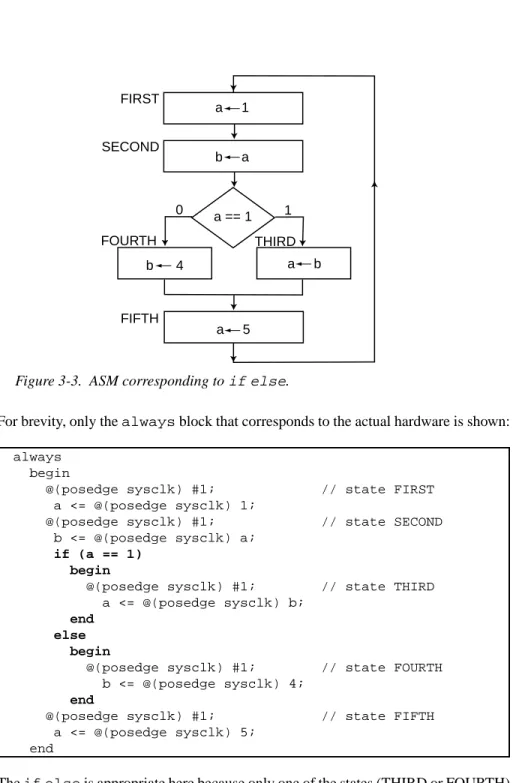
while is appropriate for a particular decision can seem confusing at first. The following ASM is an example where the ifelse construct is appropriate: Continued

(39)

For brevity, only the always block that corresponds to the actual hardware is shown:

always begin

if (a == 1) begin

end else begin

end

end

The ifelse is appropriate here because only one of the states (THIRD or FOURTH) will execute. Because a is one in state SECOND, state THIRD will execute. In the following very similar Verilog, state FOURTH rather than state THIRD will execute:

Figure 3-3. ASM corresponding to ifelse.

1 a == 1 0 a 1 b a a b b 4 a 5 FIRST SECOND THIRD FOURTH FIFTH

(40)

always begin

if (a != 1) begin

end else begin

end

3.8.2.3.4

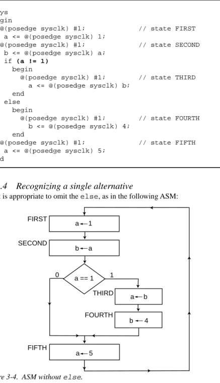
Recognizing a single alternative

Often, it is appropriate to omit the else, as in the following ASM:

Figure 3-4. ASM without else.

1 a == 1 0 a 1 b a a b b 4 a 5 FIRST SECOND THIRD FOURTH FIFTH

(41)

which translates to the following Verilog:

always begin

if (a == 1) begin

@(posedge sysclk) #1; // state THIRD a <= @(posedge sysclk) b;

@(posedge sysclk) #1; // state FOURTH b <= @(posedge sysclk) 4;

end

In the above, both state THIRD and state FOURTH will execute because a is one in state SECOND. The following very similar Verilog skips directly from state SECOND to state FIFTH:

always begin

if (a != 1) begin

end

3.8.2.3.5

Recognizing

while

loops

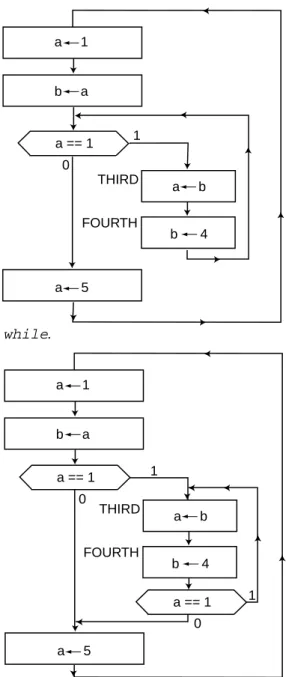
The following two ASMs describe the same hardware. The first of the following two ASMs is very similar to the one in section 3.8.2.3.4, except that state FOURTH does not necessarily go to state FIFTH . Instead, state FOURTH goes to a decision which

(42)

determines whether to go to state THIRD or state FIFTH. The second of the following two ASMs is a much less desirable way to describe the identical hardware. It is undesir-able because the a==1 test is duplicated; however, its meaning is exactly the same as the first of the following two ASMs:

Figure 3-5. ASM with while.

Figure 3-6. Equivalent to figure 3-5.

1 a == 1 0 a 1 b a a b b 4 a 5 FIRST SECOND THIRD FOURTH FIFTH 1 1 a == 1 a == 1 0 0 a 1 b a a b b 4 a 5 FIRST SECOND THIRD FOURTH FIFTH

(43)

The reason the first of the ASMs is preferred is because it is more obvious that it trans-lates into a while loop in Verilog:

always begin

while (a == 1) begin

end

In fact, the only syntactic difference between the above Verilog and the Verilog in sec-tion 3.8.2.3.4 is that the word if has been changed to while. The advantage of look-ing at this particular ASM as a while loop is that the decision a==1 is shared by both state SECOND and state FOURTH. With the while loop, the designer does not have to worry that the decision is actually part of two states. Many practical algorithms that produce useful results (as illustrated in chapter 2) demand a loop of this style. The

while in Verilog makes this easy.

3.8.2.3.6

Recognizing

forever

Sometimes machines need initialization states that execute only once. Since synthesis tools only accept behavioral Verilog defined with always blocks, such ASMs still begin with the keyword always. However, the looping action of the always is not pertinent. (If the designer only wanted to simulate the machine, initial would work just as well as always, but ultimately the synthesis tool will demand always.) In order to describe the infinite loop that exists beyond the initialization states, th