Parallel unmixing of remotely sensed hyperspectral images on commodity graphics processing units

Published online 22 March 2011 in Wiley Online Library (wileyonlinelibrary.com). DOI: 10.1002/cpe.1720

Parallel unmixing of remotely sensed hyperspectral images

on commodity graphics processing units

Sergio Sánchez, Abel Paz, Gabriel Martín and Antonio Plaza

University of Extremadura,Avda. de la Universidad s/n,10071 Cáceres,Spain

SUMMARY

Hyperspectral imaging instruments are capable of collecting hundreds of images, corresponding to different wavelength channels, for the same area on the surface of the Earth. One of the main problems in the analysis of hyperspectral data cubes is the presence of mixed pixels, which arise when the spatial resolution of the sensor is not enough to separate spectrally distinct materials. Hyperspectral unmixing is one of the most popular techniques to analyze hyperspectral data. It comprises two stages: (i) automatic identification of pure spectral signatures (endmembers) and (ii) estimation of the fractionalabundanceof each endmember in each pixel. The spectral unmixing process is quite expensive in computational terms, mainly due to the extremely high dimensionality of hyperspectral data cubes. Although this process maps nicely to high performance systems such as clusters of computers, these systems are generally expensive and difficult to adapt to real-time data processing requirements introduced by several applications, such as wildland fire tracking, biological threat detection, monitoring of oil spills, and other types of chemical contamination. In this paper, we develop an implementation of the full hyperspectral unmixing chain on commodity graphics processing units (GPUs). The proposed methodology has been implemented, using the CUDA (compute device unified architecture), and tested on three different GPU architectures: NVidia Tesla C1060, NVidia GeForce GTX 275, and NVidia GeForce 9800 GX2, achieving near real-time unmixing performance in some configurations tested when analyzing two different hyperspectral images, collected over the World Trade Center complex in New York City and the Cuprite mining district in Nevada. Copyright䉷2011 John Wiley & Sons, Ltd.

Received 17 June 2010; Revised 11 February 2011; Accepted 11 February 2011

KEY WORDS: hyperspectral imaging; endmember extraction; abundance estimation; parallel processing; GPUs

1. INTRODUCTION

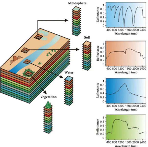
Hyperspectral imaging instruments are capable of collecting hundreds of images, corresponding to different wavelength channels, for the same area on the surface of the Earth [1]. For instance, NASA is continuously gathering imagery data with instruments such as the Jet Propulsion Laboratory’s Airborne Visible-Infrared Imaging Spectrometer (AVIRIS), able to record the visible and near-infrared spectrum (wavelength region from 0.4 to 2.5m) of the reflected light of an area 2–12 km wide and several kilometers long, using 224 spectral bands [2]. The resulting multidimensional data cube typically comprises several GB per flight (see Figure 1). The wealth of spectral information

∗_{Correspondence to: Antonio Plaza, Hyperspectral Computing Laboratory, University of Extremadura, Avda. de la} Universidad s/n, 10071 Cáceres, Spain.

Figure 1. The concept of remotely sensed hyperspectral imaging.

provided by latest generation hyperspectral sensors has opened ground breaking perspectives in many applications [3]. One of the main problems in the analysis of hyperspectral data cubes is the presence of mixed pixels [4], which arise when the spatial resolution of the sensor is not enough to separate spectrally distinct materials [5]. For instance, the pixel vector labeled as ‘vegetation’ in Figure 1 may actually be a mixed pixel comprising a mixture of vegetation and soil, or different types of soil and vegetation canopies. In this case, several spectrally pure signatures (endmembers) are combined into the same (mixed) pixel. Hyperspectral unmixing [6] is one of the most popular techniques to analyze hyperspectral data. It comprises two stages: (i) identification of endmembers and (ii) estimation of the abundance of each endmember in each pixel. The unmixing process is computationally quite expensive, due to the extremely high dimensionality of hyperspectral data cubes [7].

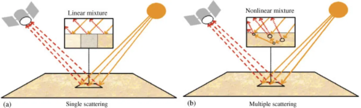
Spectral unmixing involves the separation of a pixel spectrum into its pure component endmember spectra, and the estimation of the abundance value for each endmember [4]. The linear mixture model assumes that the endmember substances are sitting side-by-side within the field of view of the imaging instrument (see Figure 2(a)). On the other hand, the nonlinear mixture model assumes nonlinear interactions between endmember substances (see Figure 2(b)). In practice, the linear model is more flexible and can be easily adapted to different analysis scenarios [6]. It can

Figure 2. Linear (a) versus nonlinear (b) mixture models in remotely sensed hyperspectral imaging.

be simply defined as follows:

r=Ea+n=

p

i=1

eiai+n, (1)

wherer is a pixel vector given by a collection of values at different wavelengths,E={ei}_i=p ₁ is a matrix containing pendmembers , a=[a1,a2,. . .,ap] is a p-dimensional vector containing the abundance fractions for each of the p endmembers in r, and n is a noise term. Two physical constraints are generally imposed into the model described in (1), these are the abundance non-negativity constraint, i.e. ai≥0, and the abundance sum-to-one constraint, i.e. _i=p ₁ai=1 [8]. Solving the linear mixture model involves: (i) identifying a collection of{ei}_ip₌₁ endmembers in the image and (ii) estimating their abundance in each pixel. Several techniques have been proposed for such purposes [4], but all of them are very expensive in computational terms. Although these techniques map nicely to high performance computing systems such as commodity clusters [9], these systems are difficult to adapt to on-board processing requirements introduced by applications, such as wildland fire tracking, biological threat detection, monitoring of oil spills, and other types of chemical contamination. In those cases, low-weight integrated components are essential to reduce mission payload. In this regard, the emergence of graphics processing units (GPUs) now offers a tremendous potential to bridge the gap towards real-time analysis of remotely sensed hyperspectral data [10–15].

In this work, we develop a new GPU implementation of a full hyperspectral unmixing chain. The proposed methodology has been implemented using NVidia’s compute device unified architecture (CUDA), and tested on three different GPU architectures and two different hyperspectral images collected by AVIRIS. The remainder of the paper is organized as follows. Section 2 describes the different modules that conform to the considered unmixing chain. Section 3 describes the GPU implementation of these modules. Section 4 presents an experimental evaluation of the proposed implementations in terms of both unmixing accuracy and parallel performance. Section 5 concludes the paper with some remarks and hints at plausible future research lines.

2. METHODS

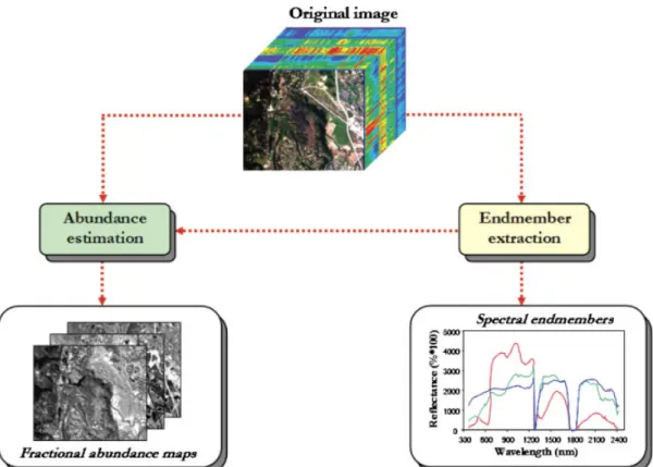
The hyperspectral unmixing chain [16] that we have implemented in this work is graphically illustrated by a flowchart in Figure 3. It should be noted that another traditional approach to implement the hyperspectral unmixing chain is based on including a dimensionality reduction step prior to the analysis. However, this step is mainly intended to reduce processing time but often discards relevant information in the spectral domain. As a result, in our implementation we do not include the dimensionality reduction step in order to work with the full spectral information available in the hyperspectral data cube. Therefore, our implementation consists of two main parts: (i) selection of pure spectral signatures or endmembers and (ii) estimation of the abundance of each endmember in each pixel of the scene.

Figure 3. Implemented hyperspectral unmixing chain.

The algorithm used in this work for endmember extraction purposes is based on the concept of orthogonal subspace projections (OSP) [17–19]. First, it calculates the pixel vector with maximum length in the hyperspectral image and labels it as an initial endmember e1 using the following expression: e1=arg max i s×l i=1 ei·eTi , (2)

wheres andl, respectively, denote the number of samples and the number of lines in the hyper-spectral image (meaning that s×l is the total number of pixels) and the superscript ‘T’ denotes the vector transpose operation. The operation ei·eTi is the dot product between a pixel vector

ei and its transposed version. The output of the dot product is a scalar value. This operation is computed for all pixels in the hyperspectral image, and the pixel vector with the maximum associated scalar value as the first endmember e1. Once an initial endmember has been identi-fied, the algorithm assigns U1=[e1] and applies an orthogonal projector [18] to all image pixel vectors, thus calculating the next endmember e2 as the pixel with maximum projection value as follows: e2=arg max i [(P ⊥ U1ei) T_(P⊥ U1ei)] with P_U⊥ 1=I−U1(U T 1U1)−1UT1, (3) where I is the identity matrix. The algorithm then assigns U2=[e1e2] and obtains the next endmembere3as follows: e3=arg max i [(P ⊥ U2ei) T_(P⊥ U2ei)] with P_U⊥ 2=I−U2(U T 2U2)−1UT2. (4)

The procedure is repeated iteratively so that a new endmember is obtained at each iteration as follows: e_j+1=arg max i [(P ⊥ Ujei) T_(P⊥ Ujei)] with P_U⊥ j=I−Uj(U T jUj)−1UTj. (5) The iterative procedure is terminated once a pre-defined number of p endmembers has been identified. The final set of endmembers,E={ei}_i=p 1, can be used to unmix a certain pixel vector ri by estimating the vectorai containing the fractional abundances of each of the pendmembers in the pixel using the technique described in [8].

3. GPU IMPLEMENTATION OF A HYPERSPECTRAL UNMIXING CHAIN

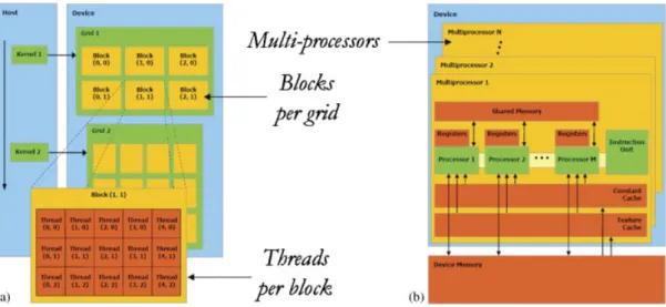
GPUs can be abstracted in terms of astream model, under which all data sets are represented as streams (i.e. ordered data sets). Algorithms are constructed by chaining so-called kernels, which operate on entire streams, taking one or more streams as inputs and producing one or more streams as outputs. Thereby, data-level parallelism is exposed to hardware, and kernels can be concurrently applied without any sort of synchronization. The kernels can perform a kind of batch processing arranged in the form of a grid of blocks, as displayed in Figure 4(a), where each block is composed of a group of threads which share data efficiently through the shared local memory and synchronize their execution for coordinating accesses to memory. There is a maximum number of threads that a block can contain but the number of threads that can be concurrently executed is much larger (several blocks executed by the same kernel can be managed concurrently, at the expense of reducing the cooperation between threads since the threads in different blocks of the same grid cannot synchronize with the other threads). Figure 4(a) displays how each kernel is executed as a grid of blocks of threads. On the other hand, Figure 4(b) shows the execution model in the GPU, which can be seen as a set of multiprocessors. Each multiprocessor is characterized by a single instruction multiple data (SIMD) architecture, i.e. in each clock cycle each processor of the multiprocessor executes the same instruction but operating on multiple data streams. Each processor has access to a local shared memory and also to local cache memories in the multiprocessor, while the multiprocessors have access to the global GPU (device) memory.

In order to implement the full unmixing procedure in a GPU, the first issue that needs to be addressed is how to map a hyperspectral image onto the memory of the GPU. Since the size of hyperspectral images may exceed the capacity of such memory, in that case we split the image

Figure 4. Schematic overview of a GPU architecture: (a) threads, blocks, and grids and (b) execution model in the GPU.

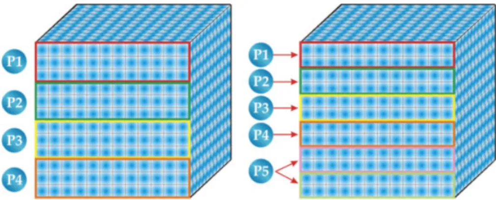
Figure 5. Spatial-domain decomposition of a hyperspectral image into four and five partitions.

into multiple spatial-domain partitions [20] made up of entire pixel vectors (see Figure 5, which shows two examples of spatial-domain partitioning of a hyperspectral image in four and five partitions, respectively). With the above ideas in mind, our GPU implementation of the hyperspectral unmixing chain comprises two stages (see Figure 3): (i) endmember extraction and (ii) abundance estimation.

3.1. GPU implementation of endmember extraction

Our GPU implementation of the OSP algorithm (called GPU-OSP hereinafter), used for endmember extraction purposes in this work, can be summarized by the following steps:

1. Once the hyperspectral image is mapped onto the GPU memory, a structure (d_image_

vector) in which the number of blocks equals the number of lines (num_lines)

in the hyperspectral image and the number of threads equals the number of samples

(num_samples) is created, thus ensuring that as many pixels as possible are processed in

parallel (see Appendix). The amount of pixels processed in parallel depends on the memory and register resources available in the GPU.

2. Using the aforementioned structure, calculate the brightest pixele1in the original hyperspec-tral scene by means of aCUDAkernel (CalculateBright), which computes (in parallel) the dot product between each pixel vectorri in the original hyperspectral image and its own transposed versionrT_i. Then, the kernelMaxBrightcalculatese1from the output provided

byCalculateBright.

3. Once the brightest pixel in the original hyperspectral image has been identified as the first endmember, the pixel (vector of bands) is allocated as the first column in theU1matrix by U1=[e1]. A kernel (called UtxU) withi blocks andithreads is now applied to calculate UT₁U1, whereiis the iteration number (between 1 and the desired number of endmembers,

p). Now the algorithm calculates the inverse of the previous product using the Gauss– Jordan elimination method [21], thus obtaining (UT₁U1)−1. A new kernel (Uxinv) with i blocks and num_bands threads is now applied to multiply U1 and the inverse of the previous step, thus obtaining U1(UT₁U1)−1. Another kernel (AnsxUt) with num_bands blocks and num_bands threads is then applied to multiply the previous result by UT₁ , thus obtainingU1(UT₁U1)−1UT₁. The subtraction of the identity matrix Iis calculated by a kernel (SustractIdentity) with num_bands blocks and num_bands threads, thus obtaining the orthogonal subspace projectorP_U⊥

1=I−U1(U

T

1U1)−1UT1. Finally, a new kernel

(PixelProjection) in which the number of blocks equals the number of lines (l) in the

hyperspectral image and the number of threads equals the number of samples (s) is applied to project the orthogonal subspace projector to each pixelri in the image (see Appendix). Finally, the maximum of all projected pixels is calculated using the kernelMaxProjection, which obtains the second endmember as follows:e2=arg{maxi[(P_U⊥₁ei)T(P_U⊥₁ei)]}.

4. The GPU-OSP now extends the reference matrixU2=[e1e2] and repeats from step 3 until the desired number of endmembers (specified by the input parameter p) has been extracted. The output of the algorithm is a set of endmembersE={ei}ip=1.

3.2. GPU implementation of abundance estimation

Our GPU version of the unconstrained abundance estimation algorithm (GPU-LSU hereinafter) uses the endmember set produced by the GPU-OSP algorithm to produce a set of endmember abundance maps as follows:

1. The first step in the GPU-LSU is to calculate a so-called compute matrix (ETE)−1ET, where

E={ei}_i=p ₁is formed by thependmembers extracted by the GPU-OSP. This compute matrix will be multiplied by all pixel vectorsri in the original image. In our implementation, the compute matrix is calculated in the CPU mainly due to two reasons: (i) its computation is relatively fast and (ii) once calculated, the compute matrix remains the same throughout the whole execution of the code.

2. The compute matrix calculated in the previous step is now multiplied by each pixelri in the hyperspectral image, thus obtaining a set of abundance vectorsai, each containing the fractional abundances of the pendmembers in each pixel. This is accomplished in the GPU by means of a kernel calledUnmixing(see Appendix).

In addition to the GPU-LSU, which does not incorporate the abundance non-negativity and sum-to-one unmixing constraints, we have also implemented partially and fully constrained abun-dance estimation algorithms. Specifically, our GPU version of the non-negative constrained linear spectral unmixing algorithm (called GPU-NCLSU) is obtained by resorting to the image space reconstruction algorithm (ISRA) [11], which imposes the abundance non-negativity constraint in abundance estimation. The algorithm guarantees convergence in a finite number of itera-tions and positive values in the abundance estimation results for any input set of endmembers. The ISRA kernel is shown in the Appendix. We have also implemented a fully constrained linear spectral unmixing algorithm (called GPU-FCLSU) by simply normalizing the abundances provided by GPU-NCLSU to provide the non-negativity and sum-to-one constraints at the same time. The CUDA kernel FCLSU that performs this operation is also displayed in the Appendix.

4. EXPERIMENTAL RESULTS 4.1. Hyperspectral image data

The first hyperspectral image scene used for experiments in this work was collected by the AVIRIS instrument, which was flown by NASA’s Jet Propulsion Laboratory over the World Trade Center area in New York City on 16 September 2001, just five days after the terrorist attacks that collapsed the two main towers and other buildings in the WTC complex. The full data set selected for experiments consists of 614×512 pixels, 224 spectral bands, and a total size of (approximately) 140 MB. The spatial resolution is 1.7 m per pixel. The leftmost part of Figure 6 shows the hyperspectral data set selected for experiments, in which vegetated areas, burned areas and smoke coming from the WTC area (in the rectangle) and going down to south Manhattan can be appreciated. Extensive reference information, collected by U.S. Geological Survey (USGS), is available for the WTC scene‡_{. In this work, we use a USGS thermal map}§ _{which shows the target}

locations of the thermal hot spots at the WTC area, displayed at the rightmost part of Figure 6. The map is centered at the region where the towers collapsed, and the temperatures of the targets range from 700 to 1020 K. Further information available from USGS about the targets (including

‡_{http://speclab.cr.usgs.gov/wtc.}

Figure 6. False color composition of an AVIRIS hyperspectral image collected by NASA’s Jet Propulsion Laboratory over lower Manhattan on 16 September 2001 (left). Location of thermal hot spots in the fires

observed in World Trade Center area (right).

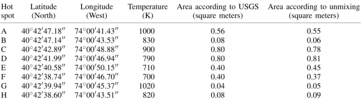
Table I. Properties of the thermal hot spots reported in the rightmost part of Figure 6.

Hot Latitude Longitude Temperature Area according to USGS Area according to unmixing

spot (North) (West) (K) (square meters) (square meters)

A 40◦4247.18 74◦0041.43 1000 0.56 0.55 B 40◦4247.14 74◦0043.53 830 0.08 0.06 C 40◦4242.89 74◦0048.88 900 0.80 0.78 D 40◦4241.99 74◦0046.94 790 0.80 0.81 E 40◦4240.58 74◦0050.15 710 0.40 0.45 F 40◦4238.74 74◦0046.70 700 0.40 0.37 G 40◦4239.94 74◦0045.37 1020 0.04 0.05 H 40◦4238.60 74◦0043.51 820 0.08 0.09

location and estimated size) is reported in Table I. As shown by Table I, all the targets are sub-pixel in size since the spatial resolution of a single pixel is 1.7 m2. The information in Table I will be used as the ground truth to validate the accuracy of the proposed parallel hyperspectral unmixing algorithms.

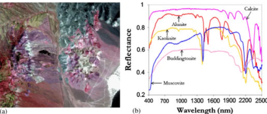
A second hyperspectral image scene has been considered for experiments. It is the well-known AVIRIS Cuprite scene (see Figure 7(a)), collected in the summer of 1997 and available online in reflectance units after atmospheric correction¶. The portion used in experiments corresponds to a 350×350-pixel subset of the sector labeled as f970619t01p02_r02_sc03.a.rfl in the online data, which comprises 188 spectral bands in the range from 400 to 2500 nm and a total size of around 50 MB. Water absorption and low SNR bands were removed prior to the analysis. The site is well understood mineralogically, and has several exposed minerals of interest, includingalunite, buddingtonite,calcite,kaolinite, andmuscovite. Reference ground signatures of the above minerals (see Figure 7(b)), available in the form of a USGS library will be used to assess endmember signature purity in this work.

4.2. Analysis of algorithm precision

Table II shows the spectral angles [18] (in degrees) between the most similar endmember pixels detected by GPU-OSP and the pixel vectors at the known target positions in the AVIRIS World ¶_{http://aviris.jpl.nasa.gov.}

Figure 7. (a) False color composition of the AVIRIS hyperspectral over the Cuprite mining district in Nevada and (b) U.S. Geological Survey mineral spectral signatures used for validation purposes.

Table II. Spectral angle values (in degrees) between the pixels extracted by GPU-OSP from the AVIRIS World Trade Center scene and the known ground-truth pixels

associated to the thermal hot spots in Figure 6.

A B C D E F G H

9.17◦ 13.75◦ 0.00◦ 0.00◦ 20.05◦ 28.07◦ 21.20◦ 21.77◦

Trade Center scene, labeled from ‘A’ to ‘H’ in the rightmost part of Figure 6. The lower the spectral angle, the more similar the spectral signatures. The range of values for the spectral angle is [0◦,90◦]. In all cases, the number of endmembers to be detected was set to p=29 after calculating the virtual dimensionality (VD) of the hyperspectral data [7]. As shown by Table II, the GPU-OSP extracted endmembers which were very similar, spectrally, to the known ground-truth pixels in Figure 6 (this method was able to perfectly detect the pixels labeled as ‘C’ and ‘D’, and had more difficulties in detecting very small targets). Finally, an evaluation of the precision of the GPU-LSU in estimating the abundance of the extracted endmembers is contained in Table I, in which the accuracy of the estimation of the sub-pixel abundance of fires in Figure 6 can be assessed by taking advantage of the information about the area covered by each thermal hot spot available from the USGS. Since each pixel in the AVIRIS scene has a size of 1.7 m2, it is inferred that the thermal hot spots are sub-pixel in nature, and thus require spectral unmixing in order to be fully characterized. In this regard, the area estimations reported in the last column of Table I demonstrate that the considered hyperspectral unmixing chain (implemented using unconstrained abundance estimation) can provide accurate estimations of the area covered by thermal hot spots. In particular, the estimations for the thermal hot spots with higher temperature (labeled as ‘A’, ‘C’, and ‘G’ in the table) are almost perfect. We have also experimentally tested that the area estimations obtained using the considered partially constrained and fully constrained abundance estimation methods are almost identical to those reported in Table I.

For illustrative purposes, Figure 8 shows the first three endmembers extracted from the AVIRIS World Trade Center scene after applying the proposed GPU-OSP implementation. If we relate the endmember plots with the three channels visible by the human eye (red, green, and blue), we can see from Figure 8 that the smoke endmember exhibits high spectral reflectance in the blue (470 nm) channel, while vegetation exhibits a peak of reflectance in the green (530 nm) channel, hence motivating that the human eye associates green color to vegetation, although the spectral signature of vegetation exhibits many other peaks and valleys. Finally, the fire endmember has high reflectance in the red (700 nm) channel, but it also shows even higher reflectance values in the short-wave infra-red (SWIR) region, located between 2000 and 2500 nm. This indicates the much higher temperature of the fires when compared to other representative endmembers in the scene.

Figure 8. Spectral endmembers of vegetation, smoke and fire extracted from the original scene by GPU-OSP.

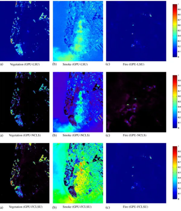
On the other hand, Figure 9 shows the abundance maps extracted for the endmembers in Figure 8 (the fire abundance maps have been rescaled to match the dimensions of the subscene displayed in the rightmost part of Figure 6, while the vegetation and smoke maps correspond to the scene displayed in the leftmost part of Figure 6). We recall that endmember abundance maps are the outcome of the unmixing process, where each map reflects the sub-pixel composition of a certain endmember in each pixel of the scene. Specifically, the maps displayed in Figure 9 correspond to vegetation, smoke, and fire. As shown in Figure 9 there are some scaling differences between the maps estimated by different unmixing methods, although the best compromise results are provided by GPU-NCLS (vegetation and fire maps with a clear separation between no abundance at all (0.0 estimated value) and high concentration of the estimated endmember) and GPU-FCLSU (good compromise result for the vegetation endmember). In turn, the GPU-LSU provides maps with fewer 0.0 estimated abundance values.

Finally, we also provide an experimental assessment of endmember extraction accuracy with the AVIRIS Cuprite scene. Table III shows the spectral angles (in degrees) between the most similar endmember pixels detected by GPU-OSP and the USGS library signatures in Figure 7(b). In this experiment, the number of endmembers to be detected was set to p=19 after calculating the VD of the AVIRIS Cuprite data. As shown by Table III, the GPU-OSP extracted endmembers which were very similar, spectrally, to the USGS library signatures, despite the potential variations (due to possible interferers still remaining after the atmospheric correction process) between the ground signatures and the airborne data. In this case, the three considered unmixing methods provide similar results. Since these results have been discussed in the previous work (see for instance [22]), we do not display them here.

4.3. GPU architectures used in our experiments

The proposed GPU implementation of the full hyperspectral unmixing chain has been tested on three different platforms:

• NVidia Tesla C1060 GPU, which features 240 processor cores operating at 1.296 GHz, with single precision floating point performance of 933 Gflops, double precision floating point performance of 78 Gflops, total dedicated memory of 4 GB, 800 MHz memory (with 512-bit GDDR3 interface) and memory bandwidth of 102 GB/s∗∗. The GPU is connected to an ∗∗_{http://www.nvidia.com/object/product_tesla_c1060_us.html.}

Figure 9. Abundance maps extracted by different GPU implementations for the vegetation (a), smoke (b), and fire (c) endmembers.

Intel core i7 920 CPU at 2.67 GHz with 8 cores, which uses a motherboard Asus P6T7 WS SuperComputer.

• NVidia GeForce GTX 275 GPU, which features 240 processor cores operating at 1.550 GHz, 80 texture processing units, a 448-bit memory interface, and a 1792 MB GDDR3 framebuffer at a 2520 MHz. It is based on the GT200 architecture††_{. The GPU is connected to a CPU Intel}

Q9450 with 4 cores, which uses a motherboard ASUS Striker II NSE (with NVidiaTM 790i chipset) and 4 GB of RAM memory at 1333 MHz.

possible algorithms: LSU, NCLSU, or FCLSU).

AVIRIS World Trade Center AVIRIS Cuprite

OSP LSU NCLSU FCLSU OSP LSU NCLSU FCLSU

Tesla C1060 Time serial (s) 757.67 33.28 3336.12 3337.32 175.31 4.79 456.71 457.03 Time GPU (s) 58.57 0.34 126.62 126.68 16.32 0.10 24.37 24.38 Speedup 12.93 97.88 26.34 26.35 10.74 47.90 18.74 18.74 GeForce GTX 275 Time serial (s) 2590.52 28.92 3402.45 3403.55 599.37 5.05 485.98 486.21 Time GPU (s) 45.51 0.77 77.16 77.18 13.53 0.26 12.49 12.49 Speedup 56.92 37.55 44.09 44.09 44.29 19.42 38.90 38.92 GeForce 9800 GX2 Time serial (s) 2590.52 28.92 3402.45 3403.55 599.37 5.05 485.98 486.21 Time GPU (s) 366.38 0.85 275.24 275.32 102.40 0.29 47.45 47.61 Speedup 7.07 34.02 12.36 12.36 5.85 17.41 10.24 10.21

• NVidia GeForce 9800 GX2 GPU, which features two G92 graphics processors, each with 128 individual scalar processor (SP) cores and 512 MB of fast DDR3 memory‡‡_{. The SPs}

are clocked at 1.5 GHz, and each can perform a fused multiply–add every clock cycle, which gives the card a theoretical peak performance of 768 Gflop/s. The GPU is also connected to a CPU Intel Q9450 with 4 cores and 4 GB of RAM memory at 1333 MHz.

4.4. Analysis of parallel performance

Before describing our parallel performance results, it is first important to emphasize that our GPU versions of OSP, LSU, NCLSU, and FCLSU provide exactly the same results as the serial versions of the same algorithms, implemented using the Intel C/C++ compiler and optimized using several compilation flags to exploit data locality and avoid redundant computations. Hence, the only difference between the serial and parallel algorithms is the time they need to complete their calculations. The serial algorithms were executed in one of the available cores, and the parallel times in each GPU platform were measured five times and the mean values are reported (these times were always very similar, with differences—if any—on the order of a few milliseconds only). The parallel times in the NVidia GeForce 9800 GX2 were measured using only one of the two G92 graphics processors available in this GPU architecture.

Table IV summarizes the obtained results in terms of parallel performance (the GPU and serial processing times are reported in each case). In all cases, the C functionclock()was used for

Figure 10. Summary plot describing the percentage of the total GPU time consumed by the different kernels used in the implementation of the GPU-OSP in the NVidia Tesla

C1060 GPU (AVIRIS World Trade Center scene).

timing the CPU implementations, and the CUDA timer was used for the GPU implementations. The time measurement was started right after the hyperspectral image file was read to the CPU memory and stopped right after the results provided by the considered algorithm are stored in the CPU memory. It should be noted that the GPU implementations have been carefully optimized taking into account the specific parameters of each considered architecture, including the global memory available, the local shared memory in each multiprocessor, and also the local cache memories. Whenever possible, we have accommodated blocks of pixels in small local memories in the GPU in order to guarantee very fast accesses, thus performing block-by-block processing to speed up the computations as much as possible. In the following, we analyze the performance of each implemented algorithm individually.

4.4.1. Parallel performance of endmember extraction. Table IV reveals that the GPU-OSP algo-rithm, used in this work for endmember extraction purposes, achieved the best speedup with regard to the serial version in the NVidia GTX 275 architecture. The lower speedup achieved in the GeForce 9800 GX2 architecture may be due to the fact that our implementation only used one of the two G92 graphics processors available in this architecture, and also because this GPU provides less processing cores than GeForce GTX 275. In this case, our results indicate that the iterative nature of the OSP algorithm requires a large number of processing cores to achieve significant speedups. Our results also indicate that the GPU-OSP can benefit from the higher processing speed of the cores in the GeForce GTX 275 compared to those available in the Tesla C1060 architecture. Also, the slightly lower speedups achieved for the AVIRIS Cuprite image (50 MB in size) compared to those obtained for the AVIRIS World Trade Center image (140 MB in size) indicate that the GPU-OSP provides more significant acceleration factors as the amount of data to be processed is larger.

For illustrative purposes, Figure 10 shows the percentage of the total GPU execution time consumed by each of the CUDA kernels (obtained after profiling the GPU-OSP implementation) along with the number of times that each kernel was invoked (in the parentheses) for the extraction ofp=29 endmembers from the AVIRIS World Trade Center scene in the NVidia Tesla C1060 archi-tecture (very similar results were also obtained in the other GPU archiarchi-tectures tested). In the figure, the percentage of time for data movements from host (CPU) to device (GPU), from device to host, and from device to device are also addressed. As shown in Figure 10, thePixelProjection

kernel consumes about 92% of the total GPU time, while MaxProjectionis the second most relevant kernel. The remaining kernels and the data movement operations are not significant (all below 1% of the total GPU time), which indicates that most of the GPU processing time is invested in the most time-consuming operation, i.e. the calculation of pixel projections and maxima scores leading to endmember identification.

4.4.2. Parallel performance of unconstrained abundance estimation. Table IV reveals that the GPU-LSU algorithm, used in this work for unconstrained linear unmixing purposes, provided

this case, the configuration of theUnmixingkernel (which receives the endmembers calculated by GPU-OSP as input) was based on allocating as many threads as pixels in the image. The idea is that each thread computes only one multiplication with the compute matrix to calculate the endmember abundances in the pixel. Before executing the Unmixing kernel, we need to load in the GPU global memory the hyperspectral image and the compute matrix. For each pixel, we perform the multiplication with the compute matrix by moving such matrix (line by line) to the shared memory in the GPU and performing the needed operations. With this scheme, we obtain a significant speedup in all cases. It is also worth noting that, as it was already the case with the GPU-OSP, the GPU-LSU provided slightly better speedups for the AVIRIS World Trade Center scene than for the AVIRIS Cuprite scene. However, in both cases the GPU-LSU provided a very fast response (in less than 1 s) for all considered GPU architectures.

For illustrative purposes, Figure 11 shows the percentage of the total GPU execution time employed by each of the CUDA kernels (obtained after profiling the GPU-LSU implementation) when unmixing the AVIRIS World Trade Center scene in the NVidia Tesla C1060 architecture. The first bar represents the percentage of time employed by the Unmixing kernel, while the second and third bars, respectively, denote the percentage of time for data movements from host (CPU) to device (GPU) and from device to host. As shown in Figure 11, theUnmixing kernel consumes about 80% of the total GPU time, while the time for data movements is not significant when compared with the time invested in performing the spectral unmixing operation.

4.4.3. Parallel performance of partially and fully constrained abundance estimation. Table IV reveals that the GPU-NCLSU and GPU-FCLSU implementations, respectively, used in this work for partially and fully constrained unmixing (and both based on the ISRA algorithm), are much more time-consuming than GPU-LSU, for all considered scenes and GPU architectures. In both algorithms, the performance increase in the GPU implementation with regard to the respective serial versions is significant, but the processing times are much larger than those reported for the GPU-LSU. This is due to the iterative nature of the ISRA algorithm (see Appendix), which imposes the non-negativity and sum-to-one constraints when solving the unmixing problem at the expense of increasing the computation time significantly. From the results in Figure 9 we can see that both NCLSU and FCLSU unmixing algorithms provide slightly more consistent results than LSU (especially for abundance values close to zero) but the increase in computational performance of these algorithms with regard to LSU makes the latter algorithm a tool of choice in many applications due to its simplicity. In any event, it is clear from Table IV that both NCLSU and FCLSU can be significantly accelerated by means of GPU implementation in any considered architecture.

For illustrative purposes, Figure 12 shows the percentage of the total GPU execution time employed by each of theCUDAkernels obtained after profiling the GPU-FCLSU implementation when unmixing the AVIRIS World Trade Center scene in the NVidia Tesla C1060 architecture. It should be noted that the GPU-NCLSU implementation is a subset of the GPU-FCLSU one, with the addition of a normalization kernel (calledFCLSU and displayed in the Appendix). The first bar represents the percentage of time employed by theISRA kernel, while the second and third bars, respectively, denote the percentage of time for data movements from host (CPU) to device (GPU) and from device to host. The reason why there are four data movements from host to

Figure 12. Summary plot describing the percentage of the total GPU time consumed by the different kernels used in the implementation of GPU-NCLSU and GPU-FCLSU in the NVidia Tesla C1060 GPU

(AVIRIS World Trade Center scene).

device is because not only the hyperspectral image but also the endmember matrix, the transposed endmember matrix, and the structure where the abundances are stored need to be forwarded to the GPU, which returns the structure with the estimated abundances after the calculation is completed. The fourth bar in Figure 12 represents the percentage of time employed by the FCLSU kernel, which is very small compared with the ISRAkernel that dominates the computations. As shown in Figure 12, theISRAkernel consumes more than 99% of the GPU time.

4.5. Real-time considerations

Before concluding the paper, it is important to emphasize that the processing times reported in the previous section are not strictly in real-time since the cross-track line scan time in AVIRIS, a push-broom instrument, is quite fast (8.3 ms to collect 512 full pixel vectors). For instance, this introduces the need to process the considered AVIRIS scene over the World Trade Center (614×512 pixels) in approximately 5.096 s to fully achieve real-time performance. It should be noted that the number of endmembers to be extracted from this scene was set to a rela-tively high number (p=29) in our experiments. However, the most relevant endmembers are always extracted by OSP in the first iterations (e.g. the fire, vegetation, and smoke endmembers in Figure 8 were the first three endmembers detected by the algorithm). As a result, reducing the value of p to extract only the most relevant endmembers can result in real-time perfor-mance of our GPU implementation of the hyperspectral unmixing chain. For illustrative purposes, Table V shows the processing times (endmember extraction plus unconstrained abundance esti-mation) measured for the AVIRIS World Trade Center scene using different values of p on the NVidia GeForce GTX 275. As shown by Table V, real-time performance is achieved for values of p≤3. A strategy that we have in mind to further speedup the performance of the unmixing chain in the task of endmember extraction is to apply a fast spectral pre-screening oper-ation to remove those pixels, which are not sufficiently pure prior to the endmember searching process implemented by OSP. In this regard, we are currently experimenting with different GPU architectures in order to fully achieve the goal of real-time endmember extraction from hyper-spectral imagery, which may allow incorporation of processing hardware onboard hyperhyper-spectral imaging instruments for real-time data exploitation at the same time as the data is collected by the sensor.

5. CONCLUSIONS AND FUTURE RESEARCH LINES

The ever increasing spatial and spectral resolutions that will be available in the new gener-ation of hyperspectral instruments for remote observgener-ation of the Earth anticipates significant improvements in the capacity of these instruments to uncover spectral signals in complex real-world analysis scenarios. Such a capacity demands parallel processing techniques which can cope with the requirements of time-critical applications and properly scale with image size, dimensionality, and complexity. In order to address such needs, in this paper we have devel-oped new GPU implementations for endmember extraction and spectral unmixing algorithms (which comprise a full hyperspectral unmixing chain). The performance of the proposed parallel algorithms has been evaluated (in terms of the quality of the solutions they provide and their

8 12 248.098 9 13 874.533 10 15 486.669 11 17 119.659 12 18 732.180 13 20 352.209 14 21 971.695 15 23 587.203 16 25 213.494 17 26 834.799 18 28 457.176 19 30 078.781 20 31 702.641 21 33 331.697 22 34 959.563 23 36 584.867 24 38 198.699 25 39 811.379 26 41 423.340 27 43 036.207 28 44 658.691 29 46 281.070

parallel performance) in the context of two real applications, using three different GPU architec-tures. The experimental results reported in this paper indicate that remotely sensed hyperspec-tral imaging can greatly benefit from the development of efficient implementations of unmixing algorithms in specialized hardware devices for better exploitation of high dimensional data sets. In this case, significant speedups are obtained using only one GPU device, with few on-board restrictions in terms of cost and size, which are important when defining mission payload in remote sensing missions (defined as the maximum load allowed in the airborne or satellite platform that carries the imaging instrument). Although the proposed implementations are not strictly in real-time for processing chains with a high number of endmembers, we expect future developments to perform in real-time mode. In order to fully substantiate the aforementioned remarks, further experimentation with additional hyperspectral scenes and GPU architectures is desirable.

APPENDIX A

In this appendix we display the code of some illustrativeCUDAkernels used in our GPU imple-mentations:

• Figure A1 shows the code for the kernelPixelProjectionused in GPU-OSP to apply an orthogonal subspace projector to each pixel in the image in order to find pendmembers.

Figure A1.CUDA kernelPixelProjectionthat applies an orthogonal subspace projector to each pixel in the image.

Figure A2. CUDAkernel Unmixing that computes endmember abun-dances in each pixel of the hyperspectral image.

Figure A3.CUDAkernelISRAthat computes endmember abundances in each pixel of the hyperspectral image imposing the abundance non-negativity constraint.

• Figure A2 shows the code for theUnmixingkernel used in the GPU-LSU implementation. This kernel calculates the pendmember abundance maps in an unconstrained fashion. • Figure A3 shows theISRAkernel used to implement the GPU-NCLSU (partially constrained

unmixing), which iteratively calculates the abundances of a set of p pre-calculated endmembers.

• Figure A4 shows theFCLSU kernel used to implement the GPU-FCLSU (fully constrained unmixing) algorithm.

Figure A4.CUDAkernelFCLSUthat computes endmember abundances in each pixel of the hyperspectral image imposing the abundance non-negativity and sum-to-one constraints.

REFERENCES

1. Goetz AFH, Vane G, Solomon JE, Rock BN. Imaging spectrometry for Earth remote sensing. Science 1985; 228:1147–1153.

2. Green RO, Eastwood ML, Sarture CM, Chrien TG, Aronsson M, Chippendale BJ, Faust JA, Pavri BE, Chovit CJ, Solis M, Monsch KA, Olah MR, Williams O. Imaging spectroscopy and the airborne visible/infrared imaging spectrometer (AVIRIS).Remote Sensing of Environment1998;65:227–248.

3. Plaza A, Benediktsson JA, Boardman J, Brazile J, Bruzzone L, Camps-Valls G, Chanussot J, Fauvel M, Gamba P, Gualtieri JA, Marconcini M, Tilton JC, Trianni G. Recent advances in techniques for hyperspectral image processing.Remote Sensing of Environment2009;113:110–122.

4. Plaza J, Plaza A, Perez R, Martinez P. On the use of small training sets for neural network-based characterization of mixed pixels in remotely sensed hyperspectral images.Pattern Recognition2009;42:3032–3045.

5. Chang C-I.Hyperspectral Imaging:Techniques for Spectral Detection and Classification. Springer: New York, 2007.

6. Plaza A, Martinez P, Perez R, Plaza J. A quantitative and comparative analysis of endmember extraction algorithms from hyperspectral data.IEEE Transactions on Geoscience and Remote Sensing2004;42:650–663.

7. Plaza A, Chang C-I.High Performance Computing in Remote Sensing(Computer and Information Science Series). Chapman & Hall/CRC Press, Taylor & Francis: Boca Raton, FL, 2007.

8. Heinz D, Chang C-I. Fully constrained least squares linear mixture analysis for material quantification in hyperspectral imagery.IEEE Transactions on Geoscience and Remote Sensing2001;39:529–545.

9. Plaza A, Chang C-I. Special issue on high performance computing for hyperspectral Imaging. International Journal of High Performance Computing Applications2008;22:363–365.

10. Paz A, Plaza A. Clusters versus GPUs for parallel automatic target detection in remotely sensed hyperspectral images.EURASIP Journal on Advances in Signal Processing2010;2010:18. Article ID: 915639.

11. De Pierro AR. On the relation between ISRA and the EM algorithm for positron emission tomography.IEEE Transactions on Medical Imaging1993;12:328–333.

12. Plaza A, Plaza J, Vegas H. Improving the performance of hyperspectral image and signal processing algorithms using parallel, distributed and specialized hardware-based systems. Journal of Signal Processing Systems2010; 50:293–315.

13. Tarabalka Y, Haavardsholm TV, Kåsen I, Skauli T. Real-time anomaly detection in hyperspectral images using multivariate normal mixture models and GPU processing.Journal of Real-Time Image Processing2009;4:287–300. 14. Setoain J, Prieto M, Tenllado C, Tirado F. GPU for parallel on-board hyperspectral image processing.International

Journal of High Performance Computing Applications2008;22:424–437.

15. Setoain J, Prieto M, Tenllado C, Plaza A, Tirado F. Parallel morphological endmember extraction using commodity graphics hardware.IEEE Geoscience and Remote Sensing Letters2007;43:441–445.

16. Plaza A, Plaza J, Paz A. Parallel heterogeneous CBIR system for efficient hyperspectral image retrieval using spectral mixture analysis.Concurrency and Computation:Practice and Experience2010;22:1138–1159.