NBER WORKING PAPER SERIES
FIXED-TERM EMPLOYMENT CONTRACTS IN AN EQUILIBRIUM SEARCH MODEL
Fernando Alvarez Marcelo Veracierto Working Paper 12791
http://www.nber.org/papers/w12791
NATIONAL BUREAU OF ECONOMIC RESEARCH 1050 Massachusetts Avenue
Cambridge, MA 02138 December 2006
We thank A. Atkeson, S. Bentolila, R. Lucas, R. Rogerson, R. Shimer, N. Stokey, J. Villaverde for their comments. The views expressed here do not necessarily reflect the position of the Federal Reserve Bank of Chicago, the Federal Reserve System, or the National Bureau of Economic Research. © 2006 by Fernando Alvarez and Marcelo Veracierto. All rights reserved. Short sections of text, not to exceed two paragraphs, may be quoted without explicit permission provided that full credit, including © notice, is given to the source.
Fixed-Term Employment Contracts in an Equilibrium Search Model Fernando Alvarez and Marcelo Veracierto
NBER Working Paper No. 12791 December 2006, Revised October 2008
JEL No. E24,J08,J3,J31,J63,J64,J65
ABSTRACT
This paper analyzes the effects of fixed-term contracts using a version of the Lucas and Prescott island model with undirected search. A fixed-term contract of length J is modeled as a tax on separations of workers with tenure higher than J . While in principle these policies require a very large state space to analyze the firms and households’ problems, we show that equilibrium allocations solve a simple dynamic programming problem. Analyzing this problem we show that equilibrium employment dynamics are characterized by two dimensional inaction sets. Finally, to understand the effect of these contracts, we compare them with two extreme cases: for J = 1 the fixed-term contracts are equivalent to the case of firing taxes, and for large J they are equivalent to the laissez-faire case. In a calibrated version of the model, we find that temporary contracts with J equivalent to three years length close about half of the gap between those two extremes.
Fernando Alvarez University of Chicago Department of Economics 1126 East 59th Street Chicago, IL 60637 and NBER f-alvarez1@uchicago.edu Marcelo Veracierto
Federal Reserve Bank of Chicago Research Department
230 South LaSalle Street Chicago, Illinois 60604 mveracie@frbchi.org
1
Introduction
This paper analyzes an undirected search version of the Lucas-Prescott (1974) model of equilibrium unemployment. This is an important extension because it combines features of the Mc Call (1970) search model (which focuses on the decision problem of an unemployed worker) with features of the Hopenhayn (1992) industry equilibrium model (which focuses on the employment dynamics of firms). The model turns out to be very tractable: In spite of the search frictions and the large amount of heterogeneity across islands we show that the optimal allocations are characterized by a simple dynamic programming problem, which we refer to as the “island planning problem”. The equivalence between these optimal allocations and two alternative equilibrium decentralizations is also demonstrated. The framework allows us to analyze an important class of policies that includesfiring taxes (as in Hopenhayn and Rogerson, 1993) and temporary employment contracts (as in Cabrales and Hopenhayn, 1997) as special cases.1 In principle, this class of policies requires
keeping track of the distribution of workers across tenure levels in each island. However, we show that the undirected search assumption leads to a state space representation that is simple enough to provide a sharp characterization of equilibrium allocations and wages.
The structure of the economy is as follows. Production takes place in a large number of locations (or islands). All islands operate the same decreasing returns to scale technology but are subject to island-specific productivity shocks. Changes in the island-specific productivity shock give raise to changes in labor demand across locations. Moving a worker across locations is costly: It requires one period during which the agent neither works nor enjoys leisure. In addition, agents that search arrive randomly to one of the islands in the economy (i.e., search is undirected). Workers that separate from their islands have to choose between two alternative activities: to work at home (i.e., to leave the labor force) or to search (i.e., to become unemployed).
The employment protection system that we consider is characterized by two parameters: the
firing taxτ and the length of thefixed-term contractsJ. Firms must pay afiring taxτ when they
1Both types of policies are common in Europe and Latin America. While firing costs have been introduced to
provide workers with employment protection, temporary contracts have been introduced as a way of giving firms
some type of flexibility in the hiring and firing process. Temporary contracts stipulate a period of time during
which workers can be dismissed at zero (or very low) cost. If workers are retained beyond this period standard separation costs apply.
reduce their employment of permanent workers (those that have a tenure level equal to or greater than J) but are exempt from payingfiring taxes on temporary workers (those with a tenure level less than J). When J = 1 this employment protection system reduces to the firing tax regime analyzed by Hopenhayn and Rogerson (1993).
We consider two alternative (yet equivalent) concepts of competitive equilibrium: one with spot labor markets and one with multiperiod employment relations. In the spot labor markets equilibrium, workers and firms solve problems that are natural extensions of the McCall (1970) search model and the Hopenhayn and Rogerson (1993) firing costs model, respectively. This equilibrium concept has two advantages: It can be easily related to the previous literature and it is simple to analyze. However, it has a considerable drawback: It assumes that the separation cost τ is triggered by the tenure level J of a worker in an island, not in an individual firm. The equilibrium with multiperiod employment relations is more complex but captures the nature of
fixed-term employment contracts in a much more realistic way. In particular, it assumes that the separation cost τ is triggered by the tenure levelJ of a worker in an individual firm.
In the spot labor market equilibrium, workers are differentiated by their tenure levels, partici-pate in different labor markets, and receive different wages. Given the presence of tenure-dependent
firing costs, firms solve a modified (S,s) optimization problem. In turn, workers at each tenure level face a standard search problem: They decide whether to stay on the island where they are currently located or become non-employed. Both firms and workers take as given the island-level law of motion for wages across tenure levels. At equilibrium, this island-level process must be such that the island labor markets clear at each island-wide state. An economy-wide equilibrium is completed by an invariant distribution across island states. This economy-wide distribution is needed to describe the benefits of search and the aggregate demand for labor.
To describe the structure of efficient allocations and their relationship with equilibrium allo-cations it is useful to consider two cases: 1) when the separation costs are a technological feature of the environment, and 2) when the separation costs are taxes rebated lump-sum to households (the interesting case to consider for policy analysis). In the first case, we show that thefirst and second welfare theorems hold. In the second case, the welfare theorems do not apply but we can still use a slightly modified version of the planning problem to characterize a competitive equilib-rium. In particular, we can break the economy-wide planning problem into a series of island-wide planning problems, one for each island. Each of these island-wide social planners solves a similar
problem: to maximize the expected discounted value of output by deciding how many workers to keep and how many workers to take out from the island. In this problem, the island-wide planner takes the constant flow U of new arrivals to the island as given (this flow is independent of the characteristics of the island because of the assumption of undirected search). The island’s planner also takes as given the shadow value of returning a worker to non-employment. This shadow value is tenure dependent, taking into account that the separation cost τ applies only to permanent workers. While the state of this problem is the distribution of workers across tenure levels, which is aJ dimensional object, we show that it can be reduced to a two-dimensional object: the number of temporary workers and the number of permanent workers. We also show that the solution to this control problem is characterized by two-dimensional sets of inaction, one set for each value of the idiosyncratic productivity shock. Given the solution to the island-wide planning problem, the economy-wide equilibrium is obtained by finding two unknowns: the equilibrium shadow value of non-employment and the equilibrium number of agents that search U.
We use our model to explore to what extent fixed-term contracts of different lengths add
flexibility to the labor market. Notice that introducingfixed-term contracts of sufficiently largeJ
is equivalent to eliminating all the separation costs (since workers never gain permanent status). Thus, we address the question of the addedflexibility by computing how much of the gap between the firing-tax case (J = 1) and the laissez-faire case (J =∞) is closed whenfixed-term contracts of empirically reasonable length are introduced. To this end we consider the case of Spain in the mid-eighties, which introduced long temporary contracts in a labor market characterized by large
firing costs. Calibrating the model to a stylized version of that economy, we find that temporary contracts of three years duration (roughly the length of the contracts introduced in Spain) close about half of the welfare gap between the firing-tax and the laissez-faire cases.
The paper is organized as follows. Section 2 relates the paper to the previous literature. Section 3 describes the economy. Section 4 defines efficient allocations. Section 5 characterizes efficient stationary allocations. Section 6 considers the two alternative notions of competitive equilibrium. Finally, Section 7 performs the computational experiments. Seven appendices contain some of the more technical analysis.
2
Related literature
This is not the first paper to introduce undirected search in the Lucas-Prescott (1974) islands model. The paper by Jovanovic (1987) is an early precursor. More recently, Alvarez and Veracierto (1999) used a similar type of structure to evaluate a number of simple policies, Veracierto (2008) considered a version with aggregate productivity shocks to analyze business cycle fluctuations, and Kambourov and Manovskii (2007) used a version with island-specific human capital to study occupational mobility. This paper differs from the previous literature in that it analyzes a different class of policies and in that it provides a systematic characterization of equilibrium and efficient allocations.
Our paper is also closely related to the literature analyzing separation taxes and temporary contracts. Within the class of papers studying separation taxes (e.g. Bentolila and Bertola, 1990, Millard and Mortensen, 1997, etc.) the general equilibrium model of Hopenhayn and Roger-son (1993) is probably the most closely related. However, our analysis extends Hopenhayn and Rogerson’s by incorporating search frictions and by evaluating the effects of separation taxes on unemployment. Within the extensive literature studying the effects of temporary contracts (e.g. Blanchard and Landier, 2002, Nagypal, 2002, etc.) the papers that are more similar in spirit to ours are Bentolila and Saint Paul (1992), Cabrales and Hopenhayn (1997), Aguiregabiria and Alonso-Borrego (2004), Veracierto (2007) and Alonso-Borrego et al. (2005), since they all study labor demand models with dynamic adjustment costs. An important difference with Bentolila and Saint Paul (1992), Cabrales and Hopenhayn (1997), and Aguiregabiria and Alonso-Borrego (2004) is that these papers consider partial equilibrium models and do not introduce unemployment. Veracierto (2007) introduces unemployment but in a partial equilibrium model with exogenous wages. In principle, Alonso-Borrego et al. (2005) is the most closely related paper since it per-forms a general equilibrium analysis with search frictions.2 However, its model is very different.
In particular, it assumes that: 1) agents face exogenous borrowing constraints, 2) employment
2Blanchard and Landier (200s2) also perform a general equilibrium analysis with search fricitions but they do
so in a framework closely related to Mortensen and Pissarides (1994), in which wages are determined through Nash
bargaining and the matching process is subject to externalities. In such a context, Blanchard and Landierfind that
introducing labor market flexibility through fixed-term contracts may lead to lower welfare levels. As we explain
contracts specify a constant wage rate as long as the employment relation lasts, 3) fixed-term contracts last only one model period, and 4) the matching process is subject to congestion ex-ternalities. While some of these assumptions are meant to provide realism, they complicate the interpretation of the results quite significantly. For instance, it is unclear to what extent the main result in the paper (which is that higher firing costs reduce unemployment and improve welfare) depends on the ad-hoc wage contracts assumed.3
In this paper we evaluate the effects of firing taxes and temporary contracts in a model with complete markets. In such a setup, government interventions cannot improve the set of mutually beneficial trades between private parties as may happen in models in which the bilateral contractual arrangements are restricted in arbitrary ways (e.g. Alvarez and Veracierto, 2001, and Alonso-Borrego, 2005). Moreover, due to convexity and lack of externalities, the laissez-faire equilibrium in our model is Pareto optimum and hence thefiring taxes and temporary contracts can only reduce welfare. In performing policy analysis in this type of setting we follow the common practice in the public finance and international trade literature of measuring Harberger triangles, i.e. of measuring the efficiency costs of the policy considered. In fact, this is also the approach that Hopenhayn and Rogerson (1993) and others have previously followed in evaluating the effects of
firing taxes.
3
Description of the Economy
Production takes place in a continuum (measure one) of different locations, or “islands.” On each island consumption goods are produced according to F (E, z), a neoclassical production function, where E is employment and z is a productivity shock that takes values in the setZ. The process for z is Markov with transition functionQ(zt+1|zt), and realizations are i.i.d. across islands. We
letf(E, z)≡∂F(E, z)/∂E and assume thatf is continuous and strictly decreasing inE, strictly increasing in z, and thatlimE→0f(E, z) =∞, where z ≡min{z :z ∈Z}.
There is a continuum of agents with mass equal toN. Agents participate in one of the following three activities: work on an island, perform home production (or, equivalently, enjoy leisure), or
3In Alvarez and Veracierto (2001), on which Alonso-Borrego (2005) is based, higher firing taxes also reduce
unemployment and improve welfare. In that setting, we show that the rigid wage contracts assumed play a crucial role in generating the results while the borrowing constraints play no important role.
search. Non-employed agents, whom we sometimes refer to as “agents being at a central location,” either work at home (enjoy leisure) or search for a job. If they work at home during the current period, they start the following period as non-employed. If a non-employed agent searches in the current period, she does not produce during the current period but arrives randomly to one of the islands at the beginning of the next period. We assume that search is undirected, so the probability of arriving to an island of any given type is given by the fraction of islands of that type in the economy. An agent located on an island at the beginning of the period can decide whether to stay on the island or become non-employed. If she stays, she works and starts the following period in the same location.
We letLt be the number of agents engaged in home production at time t, andUt the fraction
engaged in search at time t. The period utility function for the household consumingct units of
consumption goods and Lt units of leisure is the following:
u(ct, Lt) =
c1t−γ−1
1−γ +ωLt.
As it is well known, the linearity of leisure in household preferences can represent an economy with indivisible labor and employment lotteries, as in Rogerson (1988). To simplify the description of the planner’s problem, we will focus in the case where consumption and leisure are perfect substitutes, which is obtained by setting γ = 0. In this case we consider home production as an alternative activity that producesω consumption goods per period, and we let the household’s utility function simply be given by E0
P∞
t=0β
t
ct . As we explain in Section 4, this assumption is without loss of
generality, in the sense that there is a simple mapping between stationary allocations with different values of γ.
Up to this point the environment is a modification of the equilibrium search model of Lucas and Prescott (1974) that introduces household production and undirected search, as in Alvarez and Veracierto (1999). We now introduce a tenure-dependent separation cost. In this section we introduce this separation cost as being a technological feature of the environment. In Section 5 we show how to use the efficient allocation of this economy to construct an equilibrium where the separation cost is a tax levied on firms and rebated to households in a lump-sum way.
The tenure-dependent separation cost works as follows: If an agent has worked for J or more periods in a location, τ consumption goods are lost from the island’s production at the time that that worker returns to the central location. If the worker returns to the central location after less
than J periods, no separation cost is incurred. In Section 5 we present an equilibrium concept that shows that this tenure-dependent separation cost at the island level captures salient features of the temporary employment contracts used in the real world.
4
E
ffi
cient Allocations: A Formal De
fi
nition
Since the separation cost depends on tenure levels, a description of an allocation must include the distribution of workers by tenure on each island. We refer to workers with tenurej = 1, ..., J−1in a location as temporary workers and to those with tenure j ≥J as permanent workers. Thus the state of a location is given by its productivity shockz and a J dimensional vectorT indicating the number of workers with different tenure levels. In the sequential notation, locations are indexed by their state at timet = 0,denoted by X =T0. We usezt= (z
0, ..., zt−1, zt) for the history of shocks
of length t and index each location at time t by(zt, X), its history of shocks and its initial state.
The initial state of the economy is described by a distribution of locations across pairs(z0, X)and by U−1, the number of agents that searched during t = −1. We let η(X|z0) be the fraction of locations with state X conditional onz0, and q0(z) the initial distribution of z0. We assume that
q0 equals the unique invariant distribution associated with the transition function Q. We denote by qt(zt) the fraction of islands with history zt, which by the Law of Large Numbers satisfies
qt+1 ¡ zt, zt+1 ¢ =Q(zt+1|zt)qt ¡ zt¢.
We indicate the employment of agents with tenure j at a location (zt, X) by Ejt(zt, X), for
j = 0, ..., J, zt
∈Ztandt
≥0.Likewise, we denote bySjt(zt, X)the separations, i.e., the number
of agents with tenure j that return to the central location.
Formally, we say that{Ejt, Sjt, Ut, Ht}, givenηandU−1, is a feasible allocation if the following
conditions hold:
i) the island’s law of motion
Ej,t ¡ zt, X¢ = Ej−1,t−1 ¡ zt−1, X¢−Sj,t ¡ zt, X¢, j = 1,2, ..., J−1, EJ,t ¡ zt, X¢ = EJ−1,t−1 ¡ zt−1, X¢+EJ,t−1 ¡ zt−1, X¢−SJ,t ¡ zt, X¢, E0,t ¡ zt¢ = Ut−1−S0,t ¡ zt, X¢, Sj,t(zt, X)≥0fort ≥0, zt∈Zt, X ∈supp(η);
ii) the feasibility constraint for the labor market Ut+ X zt X X J X j=0 Ej,t ¡ zt, X¢qt ¡ zt¢η(X|z0) +Lt=N Ut, Lt ≥0for all t= 0,1, ...;
and iii) the initial conditions
Ej−1,−1 = Xj for j = 1,2, ..., J−1,
EJ−1,−1+EJ,−1 = XJ,
where E0,−1 =U−1.
Thefirst constraint states that the number of employed workers of tenurej ≤J−1is given by the number of workers of tenurej−1that were employed on the island during the previous period minus the number of these workers taken out of the island during the current period. The second constraint is analogous to the first constraint for workers of tenureJ or higher. It differs from the
first one because we don’t keep track of workers of tenure j ≥ J separately (they are all lumped together into tenure J). The third constraint says that the employment of tenure zero workers is given by those just arrived to the island, minus the number of them taken out of the island. The fourth constraint states that the sum of total unemployment, total employment, and agents out of the labor force equals the population N.The fifth and sixth equations defineEj,−1 in terms of the initial conditions Xj, for j = 1, ..., J.
Henceforth we defineTj,t(zt, X)as the number of workers of tenurej available at the beginning
of the period t on an island of type (zt, X), so that
Tj,t ¡ zt, X¢ = Ej−1,t−1 ¡ zt−1, X¢, j = 1,2, ..., J −1, (1) TJ,t ¡ zt, X¢ = EJ−1,t−1 ¡ zt−1, X¢+EJ,t−1 ¡ zt−1, X¢, (2) T0,t ¡ zt¢ = Ut−1 (3)
Hence condition i) in the definition of feasibility is equivalent to
Ej,t ¡
zt, X¢≤Tj,t ¡
zt, X¢ for all j.
With these objects at hand we can define a planning problem whose solutions characterize the set of efficient allocations. We say that {Ejt, Sjt, Tj,t, Ut, Lt} is an efficient allocation if it
maximizes X t βtX zt X X " F Ã J X j=0 Ej,t ¡ zt, X¢, zt ! −τ SJ,t ¡ zt, X¢ # qt ¡ zt¢η(X|z0) + X t βtωLt
over all feasible allocations, given the initial conditions η and U−1.
Given initial conditions η, U−1, a feasible allocation {Ejt, Sjt, Tj,t, Ut, Lt} is stationary if
Ut, Lt and the cross sectional distributionηt are constant over time, where ηt is given by
ηt+1(K|z0) = X zt∈Zt X X IK ¡ zt, X¢η0(X|z0)qt ¡ zt¢Q(z0|zt),
and IK is an indicator defined as
IK ¡ zt, X¢= ⎧ ⎨ ⎩ 1, if [T1,t(zt, X), ..., TJ,t(zt, X)]∈K 0, otherwise ⎫ ⎬ ⎭ for all zt ∈ Zt, X
∈ supp(η), and Borel measurable K ⊂ RJ
+. Finally, we say that {L, U, η} is a stationary efficient allocation if there is some efficient allocation nEˆjt,Sˆjt,Tˆj,t,Uˆt,Lˆt
o
with initial condition Uˆ−1, ˆη which is stationary and for which
ˆ
U−1 = ˆUt=U, Lˆt=L, and ˆηt=η for allt≥0 .
5
Characterization of E
ffi
cient Stationary Allocations
An efficient allocation is interior if agents are engaged in all three activities: search, home pro-duction, and work. Our characterization of interior efficient stationary allocations consists on the solution to two equations in two unknowns:(U, θ),whereU is unemployment and θ is the shadow value of being non-employed. One equation states that the shadow value of search equals the expected value of randomly arriving to an island next period, according to the invariant distrib-ution. The second equation ensures that agents are indifferent between doing search and home production. Thefirst equation is quite complex- it involves solving a dynamic programing problem and using the invariant distribution generated by its optimal policies. We refer to this dynamic programing problem as the island planning problem.
The state of this problem is given by (T, z), where T is a vector describing the number of workers across tenure levels j = 1,2, ..., J at the beginning of the period and z is the current
productivity shock. The island planner receives U workers with tenure j = 0 every period. The planner decides how many workers to employ at each tenure level and returns workers to the central location at a shadow value given byθ.The planner incurs a cost τ per worker with tenure
J that is returned to the central location. Formally,
V (T, z;U, θ) = max {Ej} ( F Ã J X j=0 Ej, z ! +θ Ã [U −E0] + J X j=1 [Tj−Ej] ! −τ[TJ−EJ] +βX z0 V (E0, E1, ..., EJ−2, EJ−1+EJ, z0;U, θ)Q(z0|z) )
subject to 0 ≤ Ej ≤ Tj for j = 1, .., J and 0 ≤ E0 ≤ U. We let G(T, z;U, θ) be the optimal employment decision and T0 =A(T, z) the implied transition function with T0
j+1 = Gj(T, z) for
j = 0, ..., J −2andTJ0 =GJ(T, z) +GJ−1(T, z).
It is intuitive to see that if U is the economy-wide efficient unemployment level and θ is the economy-wide shadow value of non-employment, the employment decisions of the island planners’ problem recover the economy-wide efficient employment decisions. To see why, notice that each island faces the same value forU,since search is undirected, and the same value ofθ, since workers are identical once they leave the island and arrive to the central location.
As stated above, the shadow value of non-employment is equal to the discounted expected value of randomly arriving (with zero tenure) to an island under the invariant distribution. To
find the shadow value of workers with tenure zero at each island, we define the problem of an island’s planner that faces aflow of unemployed workers equal toUˆ for one period but that reverts to the constant flowU thereafter:
ˆ V ³T, z; ˆU , θ´ = max Ej ( F Ã J X j=0 Ej, z ! +θ Ãh ˆ U −E0 i + J X j=1 [Tj −Ej] ! −τ[TJ −EJ] (4) + βX z0 V (E0, E1, ..., EJ−2, EJ−1+EJ, z0;U, θ)Q(z0|z) )
subject to 0 ≤Ej ≤ Tj for j = 1, .., J and E0 ≤ U .ˆ Using this problem we define the value of an extra zero-tenure worker in a location with state (T, z) as:
λ(T, z;U, θ) =
∂Vˆ ³T, z; ˆU , θ´
∂Uˆ |Uˆ=U (5)
where ∂V /∂ˆ Uˆ is a subgradient of Vˆ (in the case it is not differentiable). The next theorem gives a characterization of the stationary efficient allocations.
Theorem 1 . Let (U, θ) be an arbitrary pair. Let V (·;U, θ) be the solution of the island planning problem, and let G(·;U, θ), λ(·;U, θ) be the the associated optimal policies and shadow value for zero-tenure workers, respectively. Suppose that:
i) μ(·;U, θ) is a stationary distribution for the process (T, z) with transition functions given by
Q(z0|z) for z0 and A(T, z) for T0; ii) the value of search σ is given by
σ =β
Z
λ(T, z ;U, θ)μ(dT×dz ;U, θ) ;
iii) the number of agents engaged in home production L satisfies
L=N−U − Z "XJ j=0 Gj(T, z ;U, θ) # μ(dT ×dz ;U, θ)≥0;
iv) the labor force participation decisions are optimal, in the sense that
θ= max{σ, ω+βθ}, and 0 =L [θ−ω−βθ].
Finally, define η(T, z) = μ(T|z) as the distribution of T conditional on z. Then {L, U, η} is an efficient stationary allocation.
Conditions (i) and (ii) have been explained above. Condition (iii) defines the number of agents doing home production as total population minus the sum of unemployment and employment, and states that home production must be nonnegative. The first equation in condition (iv) states that the value of non-employment must be the best of two alternatives: the value of search, which is σ, and the value of doing home production during the current period and being non-employed the following period, which is ω+βθ. The second equation in condition (iv) is a complementary slackness condition for home production.
Theorem 1 implies that characterizing efficient stationary allocations is reduced to solving two equations in two unknowns and checking that an inequality is satisfied. Given an arbitrary pair (U, θ), the functions V(·, U, θ), G(·, U, θ), λ(·, U, θ), and the distribution μ(·, U, θ) can be found using standard recursive techniques. Defining σ(U, θ) andL(U, θ) as the left-hand sides of conditions (ii) and (iii), respectively, the two equations that U and θ must satisfy are:
and the inequality that must be satisfied is that L(U, θ) ≥ 0. A consequence of this simple characterization is that Theorem 1 can be used for constructing a computational algorithm and establishing the existence and uniqueness of a stationary efficient allocation.
The households’ optimality condition whenγ >0 and the allocation is interior (i.e., one with a strictly positive amount of time dedicated to leisure and a strictly positive amount of search) is to equate the marginal rate of substitution with the flow value of search:
ω
u0(c) = (1−β)σ, (6)
where cis aggregate consumption. In such interior equilibrium the value of search is equal to the value of non-employment (i.e., σ=θ).
5.1
Island Planning Problem
We now turn to the analysis of the island planning problem, which is at the center of our char-acterization. We start by analyzing the derivatives of V, which can be shown to be differentiable. The standard proof by Benveniste and Scheikman does not apply because the optimal choice of
E is not interior. In Appendix A we construct an alternative proof and find expressions for the derivatives of V. Intuitively, the marginal value of an additional worker of tenure j is given by the sum of two terms. The first term is the expected discounted sum of the marginal product of labor over periods in which no worker of the same cohort has ever been sent back to the central location. The second term is the expected discounted shadow value (net of any separation costs) the first time that a worker of the same cohort is sent back to the central location. Formally, for
Tj > 0, ∂V (T, z)/∂Tj = Vj∗(T, z), where Vj∗ is defined as follows. Denote the current date by
0 and define the stopping timenj as the first datesat which the number of workers with current
tenure j is reduced. We let E∗
i,s be the optimal employment level s periods from now of workers
with tenure level i, andTi,sbe the beginning-of-period number of workers speriods from now with
tenure level i, so that
nj = first dates at whichEmin∗ {J, j+s},s < Tmin{J, j+s},s.
Now we are ready to defineV∗
j (T, z)as: Vj∗(T, z) = ∞ X s=0 βsE0 " f à J X i=0 Ei,s∗ , zs ! |nj > s # + E0[βnj θ]−E0[βnj τ |nj ≥J] (7)
This implies that if some workers of tenure j are sent back, i.e., if Ej =Gj(T, z)< Tj, then the
marginal value of all workers of this tenure level is V∗
j (T, z) = θ for j ≤ J −1 and is equal to
θ−τ for j =J.
It can be shown that the solution to the island planning problem has the following three properties (see Appendix A for more details).
First, if Tj > 0, then ∂V (T, z)/∂Tj ≥ θ for j ≤ J and ≥ θ −τ for j = J. This must be
the case, since the planner always has the option of sending workers back to the central location (Propositions 10 and 13).
Second, if some permanent workers arefired, i.e., ifEJ =GJ(T, z)< TJ, then all the temporary
workers must have been fired, i.e., Ej = Gj(T, z) = 0 for all j = 0, ..., J −1. A policy with
this property saves on the separation cost τ, which is incurred only by the permanent workers (Proposition 11).
Third, thefirst workers to be fired are the temporary workers with the longest tenure (Propo-sition 5 and its Corollary). The intuition for this property is that, while all workers are perfect substitutes in production, these workers are the closest to becoming subject to the separation cost
τ. Thus this policy saves on potential separation costs. In an economy where all island planners have followed this policy in the past and a constant flow U of tenure j = 0 workers has arrived to each island every period, the states T in the ergodic set take a particular form. Formally, the ergodic set is a subset of E, which is given by
E =nT ∈[0, U]J−1×R+:T = (U, ..., U, Tj,0, ...,0, TJ), for some j : 1≤j ≤J−1 o
(8)
This property is extremely important: It allows us to reduce the dimensionality of the endogenous state of the island planning problem fromJ to2. The next section analyzes the resultingsimplified island planning problem.
5.2
Simpli
fi
ed Island Planning Problem
States for the island planning problemT that belong toE can be described by two numbers: t,the total number of temporary workers (workers with tenure less or equal to J), and p, the number of permanent workers (workers with tenure greater than J ). We use this feature to consider the island planning problem with a simplified state(t, p, z). In this simplified problem, the choices are
employment of temporary workersetand employment of permanent workersep.The law of motion
for the endogenous state is:
t0 =U +et−max{et−(J−1)U, 0} andp0 =ep+ max{et−(J−1)U, 0}. (9)
The number of temporary workers next period t0 is equal to the number of temporary workers
employed during the current period et plus the arrival of new workers U, minus the temporary
workers that will become permanent next period,max{et−(J −1)U, 0}. Likewise, the number of
permanent workers next period p0 is equal to the number of permanent workers employed during the current period ep plus the temporary workers that will become permanent next period. The
island planner’s value functionv: [U, J·U]×R+×Z →R satisfies the following Bellman equation:
v(t, p, z) = max et,ep,t0,p0 ½ F(et+ep, z) +θ[t−et] + (θ−τ) [p−ep] +β Z v(t0, p0, z0)Q(z, dz0) ¾ subject to 0≤et≤t, 0≤ep ≤p,
and the law of motion (9).
Formally,v is related to V for statesT ∈ E as follows:
v(T1 +T2+...+TJ−1, TJ, z) =V (T1, T2, ..., TJ−1, TJ, z).
Since v and V are closely related and V is concave, then v is concave in (t, p), even though the graph of the feasible set for this problem is not convex. From the definition ofvand the properties of V, we have thatv is differentiable with respect tot for all t >0 that are not integer multiples of U, and differentiable with respect to p for all p >0. Thus, for all(t, p, z) with p >0
∂v(t, p, z)
∂p =
∂V (T, z) ∂TJ
and for all t that can be written as t= (j−1)U+Tj with Tj ∈(0, U),
∂v(t, p, z)
∂t =
∂V (T, z) ∂Tj
.
At the points t given byt=j×U for some j = 1, ..., J −2, the right derivative of vwith respect to t is ∂V /∂Tj, and its left derivative is∂V /∂Tj+1.
The main result of this section is a characterization of the optimal policy. The optimal policy is defined by a two-dimensional set of inaction I(z). For each z, the optimal policy
(et(t, p, z), ep(t, p, z)) is to stay in the set of inaction I(z) or otherwise move to its boundary,
as explained below. The boundary of the set of inaction is described by two continuous functions,
ˆ
p and ˆt defined in pˆ : Z → R+ and tˆ: R+ ×Z → [0, J·U]. The function ˆt is decreasing in
p and hits zero at a value of p ≤ pˆ(z). The function ˆt is the boundary of the set of inaction for the values t that are strictly positive. Formally, these functions define the set of inaction I(z) as follows:
Definition 2 For each z ∈Z,
I(z) =©(t, p)∈[0, J·U]×R+ :p≤pˆ(z), and t≤ˆt(p, z)
ª
(10)
The optimal policy is as follows: if p ≤ pˆ(z) and the state is outside the set of inaction
I(z), temporary workers are fired until the boundary of I(z)is hit, with no change in permanent workers. If p > pˆ(z), all temporary workers are fired, and permanent workers are fired to hit
ˆ
p(z). Formally,
et(t, p, z) = min ©
t, tˆ(p, z)ª, and ep(t, p, z) = min{p, pˆ(z)} . (11)
The thresholdpˆ(z)solves
θ−τ =f(ˆp(z), z) +β
Z ∂v
∂p(U,pˆ(z))Q(z, dz
0)
That is,pˆis the lowest number of permanent workers for which the marginal value of a permanent worker is equal to θ−τ and, thus, any additional permanent worker would be returned to the central location.
Given (p, z), the function ˆt(p, z) is defined as the lowest number of temporary workers t for which the marginal value of a temporary worker is equal toθ and, thus, any additional temporary worker would be returned to the central location. The function ˆt(p, z)solves
θ=f¡ˆt(p, z) +p, z¢+β Z ∂v ∂t ¡ˆ t(p, z) +U, p¢Q(z, dz0) for ˆt(p, z)≤(J−1)U and θ =f¡ˆt(p, z) +p, z¢+β Z ∂v ∂p ¡ JU, p+ ˆt(p, z)−(J−1)U ¢Q(z, dz0)
for ˆt(p, z)∈((J−1)U, JU]. To simplify the exposition we have written these expressions assum-ing thatvis differentiable. Ifvis evaluated at integers multiples ofU (wherevis not differentiable), the expressions would have to be rewritten in terms of the subgradients of v.
The intuition for why the frontier of the set of inaction, given by ˆt, is decreasing in p is that temporary and permanent workers are perfect substitutes in production. Indeed, it can be shown that ˆt is strictly decreasing for values ofpsuch thattˆ(p, z) is not an integer multiple ofU.At the points on whichtˆis an integer multiple ofU, this function can beflat: At these points the function
v may not be differentiable, as explained above. While all these properties are quite intuitive, the proofs are involved because of the non-differentiability of v (Appendix B provides more details).
The optimal decision rule for the island planning problem generates considerable churning of temporary workers. To see that this is the case, consider an island in a state (t, p, z) satisfying that p ≤ pˆ(z) andt ≥tˆ(p, z). From equation (11) we know that such an island employs ˆt(p, z)
temporary workers and p permanent workers. Since the island receives U new workers every period it follows that, as long as its productivity level remains at z, its state will be given by
¡ˆ
t(p, z) +U, p, z¢ and it will employ ˆt(p, z) temporary workers and p permanent workers. From Section 5.1 we know that the first temporary workers to be sent back to the central location are those with the longest tenure. Thus, as long as the productivity level remains at z, the
island’s planner keeps replacingU temporary workers with the longest tenure with the new arrivals. Observe that the undirected search assumption is crucial for obtaining this result: If search was directed all new arrivals would be at islands that expand their employment levels and, therefore, no churning of temporary workers would take place.
6
Competitive Equilibrium
The representative household has a continuum of members that share their employment risks. Given the perfect consumption pooling at the household level, each household member seeks to maximize her own expected discounted earnings regardless of risk.4
In what follows it will be useful to think of each island as a separate economy and define an “island-level equilibrium,” taking as given the flow of new workers to the island, U, and the value to a worker of leaving the island, θ. The resulting equilibrium decision rules at the island level define an invariant distribution across island states, which together with U and θ must satisfy certain conditions to constitute an “economy-wide equilibrium.” These conditions are that the consumption market clears, the labor market clears, and the marginal rate of substitution between consumption and leisure equals the flow value of search.
In this section we describe two notions of island-level equilibrium: one with spot labor markets (SLM) and one with multiperiod employment relations (MER). The SLM specification has two advantages: 1) It makes a straightforward connection with the island planning problem, and 2) it is closely related to the standard McCall search model (on the workers’ side) and to the Hopenhayn and Rogerson’s firing costs model (on thefirms’ side). The advantage of the MER specification is that it captures the nature of fixed-term employment contracts in a much more realistic way.
Appendix C gives a formal definition of a SLM equilibrium, relates it to the island planning problem of Section 4 and characterizes the behavior of equilibrium wages. Appendix D provides a similar analysis for a MER equilibrium.
In this section and most of appendices C and D we assume that γ = 0 (so that consumption and leisure are perfect substitutes) and that the separation cost τ is a feature of the technology
4An equivalent specification would be to identify each household with one individual and introduce complete
markets and employment/search lotteries, as in Prescott and Rios-Rull (1992). However, this alternative would require introducing additional notation.
(as opposed to a tax rebated lump-sum to households). The first assumption is used to simplify the description of an equilibrium. The second is used to show that the first and second welfare theorems hold.
Whenγ ≥ 0and τ is a tax, the equilibrium allocation satisfies the same conditions described in Theorem 1, except thatL ∈(0, N),ω is replaced byω˜ =ω / u0(c), and aggregate consumption
c is given by the integral of output under the invariant distribution μ (without subtracting the separation taxesτ). It turns out that for Cobb-DouglasF and CRRAu, an equilibrium allocation can always be obtained by re-scaling the efficient allocation (that satisfies conditions (i)-(iv) in Theorem 1) by some appropriate factor.
6.1
Spot Labor Markets
In an SLM equilibrium, firms and workers participate in competitive labor markets on each island. Wages are indexed by j, the workers’ tenure on the island and by (T, z), the island-wide state. As in the previous sections, a permanent worker is defined as having tenure j ≥J on the island. Whenever a firm decreases its employment of permanent workers, it must pay a separation cost
τ per unit reduction. Notice that it is the tenure at the island level, as opposed to the tenure at the firm level, that determines if a worker separation is subject to the separation cost τ. This unrealistic assumption affords tractability by allowing a decentralization with spot labor markets. The reason is that, since the separation costs are at the island level, workers are not tied to the
firms that hire them.
In an SLM equilibrium, a worker located on an island at the beginning of the period solves a very simple problem: whether to stay on the island, receive the wage rate corresponding to her tenure level and start the following period with a higher tenure level, or to leave, in which case she can either search or engage in home production. This problem also applies to workers who have just arrived at an island (i.e., with zero-tenure level). Moreover, in equilibrium searchers contact an island in proportion to its frequency in the invariant distribution. Hence, the problem for searchers is the same as in the classical McCall search model, except that wages depend on tenure levels and the wage distribution is endogenous.
The problem for a firm in an SLM is similar to the one studied by Hopenhayn and Rogerson (1993): Firms take the stochastic process for wages as given, behave as if they could hire and fire
any number of workers at these wages, and are subject to a cost τ per reduction of employment. One difference is that in our formulation the separation costτ applies only to workers with tenure
j ≥ J on the island, as opposed to all workers. Another difference is that the process for wages at the island level is endogenously determined: The process for the island-level equilibrium wages must be such that the demand for labor equals its supply at each tenure level and island-wide state.
Since workers and firms take competitive wages as given, the equilibrium pattern of wages across tenure levels must inducefirms and workers to follow the employment adjustments described in Figure 2. Proposition 36 in Appendix C shows that there are three equilibrium levels of wages in a given location: one level for temporary workers with tenuresj = 0, ..., J−2,a second level for workers that are about to become permanent, i.e., those with tenure J−1, and a third level for permanent workers, i.e., those with tenure J or higher. Temporary workers with tenures j = 0 to
j =J−2are paid their marginal productivity. Wages of workers with tenureJ−1, i.e., those that would become permanent if they were to work during the current period, are (weakly) smaller than their marginal productivity. Wages of permanent workers are (weakly) higher than those with tenure J−1.
6.2
Multiperiod Employment Relations
In the previous sections the separation cost τ applied to workers with tenure j ≥J at the island level, which allowed for a simple competitive structure with spot labor markets. In this section we introduce an alternative and more realistic definition of a competitive equilibrium, where separation costs are determined by the tenure of workers at the firm level. This specification ties workers with firms and, hence, requires long-term contracts to achieve efficiency. In fact, we will argue that the competitive equilibrium with long-term contracts and tenure at the firm level supports the same equilibrium allocation as the spot labor market concept of the previous section. This is an important result: There is no loss of realism in specifying that the relevant tenure for temporary contracts is at the island level rather than at the firm level.
To obtain this equivalence result certain restrictions on the type of temporary contracts allowed for are needed. However, this is not a weakness of the model: These restrictions resemble those observed in actual countries. Indeed, since temporary contracts are often introduced with the
purpose of increasingflows out of unemployment, their implementation typically includes eligibility clauses. An example is the Spanish reform of 1984, which significantly broadened the scope of
fixed-term contracts but specified that workers had to be registered as unemployed to be eligible for temporary employment contracts (see the Appendix in Cabrales and Hopenhayn, 1997). In Portugal temporary contracts could only be used by new firms, or by firms hiring long-term unemployed or first-time job seekers (see Table 1 in Dolado et al., 2001). Another example is the recently approved and later withdrawn CPE (“first employment contract”) legislation in France. This type of contract would have allowed an employer to dismiss a worker younger than 25 during the first two years of the contract, provided that he had never been employed at the time of his hiring
To incorporate this type of eligibility restriction we assume that only workers that searched during the previous period (i.e., that were unemployed) can be hired under temporary contracts. If a firm hires a worker that was employed somewhere else on the island during the previous period, the worker immediately becomes subject to regular firing taxes. In this scenario, the market structure would have to be changed to accommodate the fact that workers would try to exploit the bargaining power that they would gain by staying in the same firm. To avoid this, we assume that firms and workers participate in island-wide competitive markets for binding, long-term, state-contingent, wage contracts at the time of the hiring. Below we offer an informal description of the equilibrium using long-term contracts. Appendix D provides a formal treatment. In this decentralization,firms and workers trade state contingent contracts in competitive labor markets, specifying the periods of time that the worker will supply labor to the firm as a function of the sequence of productivity shocks zt. Since employment must be continuous over time, each
contingent contract is effectively reduced to a stopping time specifying the time of separation. When the realized sequence of productivity shocks triggers a separation, the worker can choose to offer a new stopping time to the market or to leave the island and receive the outside value θ. Each stopping time has its own price, which is taken as given by firms and workers.
There are two types of workers on the island: “incumbent” workers and “newly arrived” workers. An “incumbent” is a worker that has been previously employed by some firm on the island. A “newly arrived” worker is a worker that has just arrived at the island for the first time. The stopping times sold by different types of workers differ in terms of the separation costs involved. In particular, the stopping times sold by “newly arrived” workers are subject to the separation
cost τ only if the separation occurs after J periods (the length of the trial periods in the fi xed-term contracts). On the contrary, the stopping times sold by “incumbents” are always subject to the separation cost τ. Since the stopping times sold by the different types of workers are different commodities, they have, in general, different prices. Intuitively, a stopping time sold by an “incumbent” worker will have a lower price than the same stopping time sold by a “newly arrived” worker to compensate firms for the potentially higher separation costs.
Taking prices as given, firms decide how many stopping times of each type to purchase from the different types of workers. Their objective is to maximize the expected present value of their profits, net of separation costs.
Despite the unusual commodities traded and the indivisibility in the supply of contracts, the competitive equilibrium considered is standard and, hence, the welfare theorems hold. The equi-librium allocation can then be characterized as the solution to a social planner’s problem. In this problem, the planner chooses stopping times for “incumbents” and “newly arrived” workers taking into account that the separation cost τ applies to “incumbent” workers in every separation, but that it applies to “newly arrived” workers only in separations that take place after J periods of employment.
A brief analysis of the planner’s problem will help us to understand the equivalence between this type of equilibrium and the SLM equilibrium of the previous section. To start with, note that the social planner will never want to separate a “newly arrived” worker and rehire him as an “incumbent” before the trial period for the fixed-term contracts is over. The reason is that being rehired as an “incumbent” makes the worker liable to separation costs, while maintaining his “newly arrived” status saves on separation costs during the trial period. Also, the social planner will never want to separate a “newly arrived” worker after the trial period is over and rehire him under an “incumbent” contract because this entails incurring the separation cost τ without any benefit. As a consequence, the planner will choose the stopping times for “newly arrived” workers in such a way that they separate only to leave the island (and receive the value θ). This means that the social planner will never use “incumbent” workers. Being left with only “newly arrived” workers, the planner’s problem is formally identical to the island planning problem described in Section 4. This has an important implication: The allocation obtained in the MER equilibrium (with tenure at thefirm level) is identical to the one obtained in the SLM equilibrium (with tenure at the island level). Moreover, the price of a stopping time sold by a “newly arrived” worker in
the MER equilibrium must be equal to the expected discounted value of the spot wages obtained by a “newly arrived” worker in the SLM equilibrium.
7
Computational Experiments
In this section we evaluate to what extent the introduction of temporary contracts adds flexibility to the labor market. To this end we consider as a benchmark the case where J = 1 and τ > 0
and calibrate it to an economy with high separation taxes and no temporary contracts.5 Once the benchmark economy (hereafter referred to as the “firing-tax” case) is parameterized, we com-pute competitive equilibria under temporary employment contracts of different lengths (i.e., with different values for J) and evaluate their effects.
For comparison purposes we also compute the equilibrium allocation under zero separation taxes, which we refer to as the “laissez-faire” case. This is an interesting case to consider because the equilibrium allocation with temporary employment contracts of long duration coincides with the equilibrium allocation under laissez-faire. The reason is quite simple: With a large enoughJ,
firms can perfectly replicate their laissez-faire employment levels by using only temporary workers. Given this property, we address the question of how much flexibility the temporary contracts generate by computing what fraction of the gap between the firing-tax and laissez-faire cases is closed when temporary contracts of different length J are introduced.
We note that in the laissez-faire case, which is obtained by setting τ = 0, the value of J and the tenure levels of different workers are immaterial because temporary and permanent workers become perfect substitutes. This implies that, while total employment is uniquely determined, the hiring andfiring rates across the different tenure levels are undetermined. Despite this, we choose to focus on the employment adjustments obtained as the limit when τ →0(or equivalently, when
τ is arbitrarily small). This is useful because it helps emphasize the types of adjustments that temporary contracts lead to even in the case in which they are totally unimportant.
The section is divided into three parts: The first part motivates the computational exercise with empirical observations, the second part calibrates the model, and the third part reports the
5When J = 1, the dismissal of anyone that has worked, even for one period, triggers the separation tax
results.
Some empirical background
Since the introduction of fixed-term contracts during the 1980s, the fraction of workers hired under this modality has expanded steadily in Europe, reaching more than 13 percent in 2000. However, there are large cross-country differences in the scope and duration offixed-term contracts. For instance, some countries restrict these contracts to certain occupations and type of workers, while others give them broad applicability. In what follows we focus on the case of Spain, because in 1984 Spain substantially liberalized the applicability of temporary contracts at a time when the country had one of the highest employment protection levels in Europe (see Cabrales and Hopenhayn, 1997, and Heckman and Pages-Serra, 2000). From 1984 to 1991, the fraction of workers with fixed-term contracts in Spain went from 11 percent to more than 30 percent, and almost all the hiring in the economy was done under this form of contract (see Hopenhayn and Garcia-Fontes, 1996).6
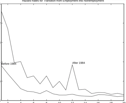
Figure 2, which is taken from Cabrales and Hopenhayn (1997), displays estimates for the one-quarter transition probabilities from employment to unemployment during the six years before and after the 1984 reform, as a function of the length of the employment spells. It shows that thefiring rates increased significantly after the reform and that a spike formed at an employment duration of three years, which (not surprisingly) corresponds to the maximum fixed-term contract length allowed by the reform. Thus, the introduction of fixed-term contracts appears to have significant effects on worker reallocation. In fact, there is considerable agreement in the empirical literature that the main effects of introducing fixed-term contracts are a substantial increase in the flows from unemployment to employment (i.e., a decrease in the average duration of unemployment), and a significant increase in theflows from employment to unemployment (i.e., an increase in the
firing rate) as can be seen, for example, in the literature survey by Dolado et al. (2001). The net effect of these two opposing forces on the unemployment rate is not clear, but the evidence seems to indicate a small increase.
6These reforms were partially undone during the 1990s, when the maximum length of thefixed-term contracts
was reduced from three years to one year, and the severance payments for ordinary indefinite-length contracts were
substantially reduced. However, even after this partial reversal, the fraction of workers underfixed-term contracts
2 4 6 8 10 12 14 16 18 20 0 0.05 0.1 0.15 0.2 0.25
FIGURE 2: Firing Rates in Spain
Hazard Rates for Transition from Employment into Nonemployment
Quarters of tenure
Percentage fired over employment, by tenure in the firm
After 1984 Before 1984
From Table 9, Cabrales and Hopenhayn 1997
Calibration
We calibrate our model to the Spanish economy prior to the 1984 reform, which (as was mentioned above) was characterized by high separation costs and no temporary contracts (i.e., high τ and J = 1). The value for τ is selected to reproduce the expected discounted dismissal cost when a worker is hired for the first time, a measure proposed by Heckman and Pages-Serra (2000). It turns out that a value of τ equal to one year of average wages is needed to reproduce this measure under the pre-1984 Spanish regime (see Appendix E for details).
We useα = 0.64for the curvature parameter in the production functionF(E, z) =zEα, which roughly corresponds to the labor share. This choice implicitly assumes that all other factors, such as capital, are fixed across locations. Since we use a quarterly time period, we chooseβ = 0.96to generate an annual interest rate of 4 percent.
For the idiosyncratic shocksz, we use a discrete Markov chain approximation to the following AR(1) process: logz0 =ρlogz+σε, whereε is a standard normal. We choose the values of ρand
σ so that the unemployment rate is just above 6.75 percent and the duration of unemployment is just above one year. The exact values that we use areρ= 0.955 andσ2 = 0.075, which correspond to a discrete approximation that uses six truncated values for z, so that the absolute value of
(total separations divided by employment) in the benchmark case is 1.77 percent. By contrast, Garcia-Fontes and Hopenhayn (1996) estimate a firing rate of 1.84 percent per quarter for the years 1978-1984. Observe that our choices are meant to capture the situation in Spain before the 1984 reform. The reason why we choose a lower unemployment rate and a lower duration of unemployment than those observed in Spain is that we are abstracting from its unemployment insurance system.7
We consider different values of γ. In each case we pick the value of ω so that labor force participation equals 65 percent in the benchmark case.8 The rest of the parameters are the same
for each pair (γ, ω).
Experiments
We compute equilibria under different values ofJ, the length of the temporary contracts, and compare them with the benchmark and laissez-faire cases. Since these two cases correspond to
J = 1andJ =∞, respectively, these comparisons allow us to determine what fraction of the total potential gains in labor market flexibility is realized by different temporary contracts lengths.
As we vary the value of J we set τ to the same proportion of economy-wide wages. For reasons outlined at the beginning of Section 5, if F is Cobb-Douglass and τ is proportional to economy-wide wages, a number of statistics become independent of the intertemporal substitution parameter 1/γ. In particular, the unemployment rate, the average duration of unemployment, and the firing rates are the same in all cases. For this reason, we start by describing the effects of temporary contracts on this set of statistics. Without loss of generality we set γ = 0. This is the simplest case to interpret because consumption and leisure become perfect substitutes and, as a consequence, the equilibrium value of θ must be equal to ω/(1−β), a parameter independent of policy.
7In Alvarez and Veracierto (1999) we analyzed the effects of introducing unemployment insurance benefits into
the model withfiring taxes. Introducing UI benefits of the magnitude of those in Spain increases the unemployment
rate by more than 10% and more than doubles its average duration (see section “UI benefits,firing subsidies,firing taxes and severance payments” and Table 5 of Alvarez and Veracierto, 1999).
8The different combinations of (γ, ω) are: (0, 1.3047), (1/2, 1.0739), (1, 0.883) and (8, 0.058). With γ =
0, there are no income effects, since preferences are linear. With γ = 1, income and substitution effects of a
permanent increase in wages cancel. With γ = 8, the income effect is much higher, so that the uncompensated
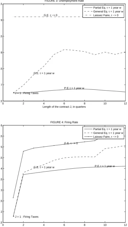
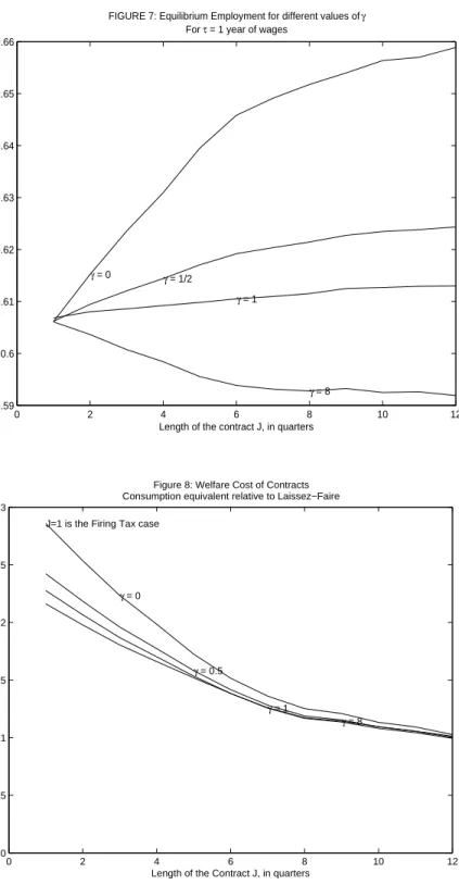
In Figures 3-5, equilibrium values are reported as a function of the length of the temporary contracts J and depicted under the “general equilibrium” label. Observe that the “general equi-librium” values for J = 1 correspond to the benchmark case with firing taxes and no temporary contracts. Laissez-faire values are reported under the “laissez-faire” label. In addition, to illus-trate the role of general equilibrium effects in generating differences between the benchmarkJ = 1
and the laissez-faire cases, a third set of values is reported under the “partial equilibrium” label. For each J >1, these are the values associated with the solution to the island planner’s problem when theU andθ that the planner takes as given are the ones from the benchmark case. Observe that any differences between the “partial” and “general” equilibrium schedules must be due to equilibrium effects on U, since θ is fixed when γ = 0. Also observe that U will always be higher in the “general equilibrium” case than in the “partial equilibrium” case. The reason for this is that with J > 1 there are fewer restrictions to labor mobility. This increases the shadow value of an additional worker at every island and induces a larger fraction of the population to search.9 For similar reasons, the equilibrium value of U will always be increasing with J. A consequence of this is that for 1< J < ∞, the equilibrium value of U will always lie between the benchmark and laissez-faire cases.
Figure 3 shows the effects on the unemployment rate ur = U/(U +E). We see that the unemployment rate increases with the length of the temporary contracts J and is almost 2.5 percent higher in the laissez-faire case than in the benchmark J = 1 case. With temporary contracts of three years duration (J = 12), the unemployment rate is 1.3 percent points higher than in the benchmark case. Temporary contracts of this length, which are similar to those introduced by the 1984 Spanish reform, are thus able to close about half of the gap with the laissez-faire case.10 Figure 3 also shows that the equilibrium effects onU are crucial for generating
the higher unemployment rates: The effects on the unemployment rate are non-monotonic and small in the partial equilibrium case.11
9Because of the decreasing returns to scale at the island level, the higher value forU reduces the shadow value
of an additional worker at every island and restores the general equilibrium.
10In the data the relationship between unemployment and temporary contracts is not as clear. However, Dolado
et al. (2001) survey the literature and conclude that the introduction of temporary contracts in Spain had a
“neutral or slightly positive effect on unemployment.”
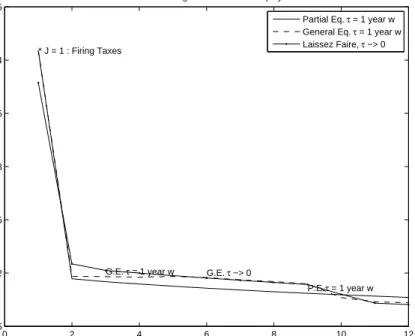
To better understand the effects on the unemployment rate (Figure 3) it is helpful to decompose them into firing rate effects (Figure 4) and average duration of unemployment effects (Figure 5). Figure 4 shows the effects on the firing rate f r, defined as total firing over total employment. Recall that for the laissez-faire and the partial equilibrium cases, the values of U and θ are the same across allJ.As it should be expected, thefiring rates for laissez-faire are higher than the ones for the partial equilibrium case for all values of J. Notice that the firing rates in these two cases are increasing in J,with a large jump atJ = 2.To understand this pattern we concentrate on the laissez-faire case where the employment on each island stays constant. Recall that we compute employment by tenure in the laissez-faire case as the limit for an equilibrium with τ → 0. The increase in the firing rate helps to avoid the (arbitrarily small) separation tax. The firing rate jumps betweenJ = 1and J = 2 because, with J = 2, the temporary workers with longest tenure arefired and replaced by newly arrived workers. This reshuffling cannot be done with J = 1.The smooth increase in thefiring rate withJ is due to the fact that with higherJ,firms can accumulate a larger proportion of their work force as temporary workers. With this larger proportion, if they need to decrease total employment they can do so at the same time that they hire newly arrived workers. Notice that the pattern of firing rates as a function of J for the partial equilibrium case where the separation costs are substantial (one year of average wages) is the same as in the laissez-faire case, with essentially zero firing taxes.
problem is similar to the standard problem of a firm facing firing costs (except that its hiring is bounded above
by the arrival of new workersU) and we know at least since Bentolila and Bertola (1990) that the effects offiring
0 2 4 6 8 10 12 6.5 7 7.5 8 8.5 9 9.5
FIGURE 3: Unemployment Rate
Length of the contract J, in quarters
Unemployment Rate, in %
* J = 1 : Firing Taxes
G.E. τ = 1 year w G.E. τ −> 0
P.E. τ = 1 year w
Partial Eq. τ = 1 year w General Eq. τ = 1 year w Laissez Faire, τ −> 0 0 2 4 6 8 10 12 1.5 2 2.5 3 3.5 4 4.5 5 5.5 6
FIGURE 4: Firing Rate
Length of the contract J, in quarters
Firing as % of employment
* J = 1 : Firing Taxes
G.E. τ = 1 year w
G.E. τ −> 0
P.E. τ = 1 year w Partial Eq. τ = 1 year w General Eq. τ = 1 year w Laissez Faire, τ −> 0
The value for the firing rate in the general equilibrium case lies in between the value for the partial equilibrium case and the one for the laissez-faire case, and it gets closer to the one for the laissez-faire case as J increases. Since in general equilibrium firms receive a higher flow of newly arrived workers (i.e., a higher U), they can engage more in the replacement of temporary workers with high tenure for newly arrived workers to save on separation costs.
5.1 percent forJ = 12,roughly similar to the values for Spain before and after 1984: Garcia-Fontes and Hopenhayn (1996) estimate quarterly firing rates of 1.84 percent during the six years prior to the extension of temporary contracts and 4.8 percent for the six years after. The model slightly overestimate these effects, since comparing the effect in the model for J = 1 withJ = 12does not correspond exactly to Spain before and after 1984 – before 1984 some temporary contracts were allowed, as we explain below.
Figure 5 shows the average duration of unemploymentd, defined as(1/f r) ur /(1−ur). The three cases display similar values. There is a large drop in the average duration between the benchmark case andJ = 2.This is the result of the increase in hiring of newly arrived workers, as explained in the case of Figure 4. Sincedis similar for the three cases, the effects on unemployment are accounted by the behavior of firing rates discussed above. Notice that, as opposed to the jumps at J = 2 for the firing rate and average duration of unemployment, the increase in the unemployment rate for the general equilibrium is smooth (compare Figure 3 with Figures 4 and 5). This is because for J = 2, the sharp decrease in the average duration of unemployment coincides with a sharp increase in the firing rate.
0 2 4 6 8 10 12 1.5 2 2.5 3 3.5 4 4.5
FIGURE 5: Average Duration of Unemployment
Length of the contract J, in quarters
Average Duration, in quarters
* J = 1 : Firing Taxes
G.E. τ = 1 year w G.E. τ −> 0
P.E. τ = 1 year w Partial Eq. τ = 1 year w General Eq. τ = 1 year w Laissez Faire, τ −> 0
0 2 4 6 8 10 12 0.65 0.7 0.75 0.8 0.85 0.9 0.95 1
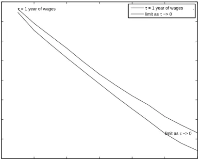
FIGURE 6: Share of Permanent Workers in Total Employment for differentg contract length J
Length of the contract J, in quarters
Permament Workers Employment / Total Employment
τ = 1 year of wages
limit as τ −> 0
τ = 1 year of wages . limit as τ −> 0
Figure 6 displays the fraction of permanent workers in total employment for the general librium and laissez-faire cases. The fraction of permanent workers is higher for the general equi-librium case than for the laissez-faire case, since in the general equiequi-librium case firms retain more permanent workers to avoid the high separation cost. Nevertheless, the fraction of permanent workers is very similar in the two cases. Notice also that asJ increases, the fraction of permanent workers decreases steadily. For J = 12,which corresponds to temporary contracts of three years, 33 percent of workers are in temporary contracts. In Europe in the 1990s, the fraction of workers with temporary contracts increased steadily over time to about 12 percent, reaching its highest value in Spain; there this fraction went from 11 percent before 1984 to an average of 33 percent during the 1990s.
Notice that the patterns displayed in Figures 5 and 6 for the average duration of unemployment and the share of permanent workers in total employment are similar to the ones found in Spain after the mid-1980s and have typically being interpreted as evidence that temporary contracts play an important role. However, in our model similar patterns are obtained for τ equal to one year of average wages as well as for τ arbitrarily small, which shows that by itself, large changes in turnover do not necessarily entail large changes in welfare and other relevant variables, such as employment, unemployment, aggregate consumption and productivity. We obtain this result under the extreme assumption that workers with different tenure are perfect substitutes. Under a