Testing conditional factor models
∗
Andrew Ang
†Columbia University and NBER
Dennis Kristensen
‡UCL and IFS
This Version: 20 February, 2012
JEL classification: C12, C13, C14, C32, G12.
Keywords: Nonparametric estimator; Time-varying beta;
Conditional alpha; Book-to-market premium; Value and momentum.
∗We thank Pengcheng Wan for research assistance and Kenneth French for providing data. For helpful comments and suggestions, we thank an anonymous referee, Matias Cattaneo, Will Goetzmann, Jonathan Lewellen, Serena Ng, Jay Shanken, Masahiro Watanabe and Guofu Zhou, as well as seminar partici-pants at Columbia University, Dartmouth University, Georgetown University, Emory University, Federal Reserve Board, Massachusetts Institute of Technology, Oxford-Man Institute of Quantitative Finance, Princeton University, State University in New York at Albany, Washington University in St. Louis, Yale University, University of Montr´eal, the American Finance Association 2010 meeting, the Banff Interna-tional Research Station 2009 Conference on ”Semiparametric and Nonparametric Methods in Economet-rics”, the Econometric Society Australasian 2009 meeting, the Humboldt-Copenhagen 2009 Conference on ”Recent Developments in Financial Econometrics”, the 2010 National Bureau of Economic Research Summer Institute, and the New York University Five Star 2009 conference. Andrew Ang acknowledges funding from the Network for Studies on Pension, Aging and Retirement (Netspar). Dennis Kristensen acknowledges funding from the Danish National Research Foundation through a grant to Center for Re-search in Econometric Analysis of Time Series (CREATES) and the National Science Foundation (grant no. SES-0961596). Corresponding author: Dennis Kristensen
†Email: [email protected] ‡Email: [email protected]
Abstract
Using nonparametric techniques, we develop a methodology for estimating and testing condi-tional alphas and betas and long-run alphas and betas, which are the averages of condicondi-tional alphas and betas, respectively, across time. The estimators and tests can be implemented for a single asset or jointly across portfolios. The traditional Gibbons, Ross, and Shanken (1989) test arises as a special case of no time variation in the alphas and factor loadings and homoskedastic-ity. As applications of the methodology, we estimate conditional CAPM and multifactor models on book-to-market and momentum decile portfolios. We reject the null that long-run alphas are equal to zero even though there is substantial variation in the conditional factor loadings of these portfolios.
1
Introduction
Under the null of a factor model, an asset’s expected excess return should be zero after con-trolling for that asset’s systematic factor exposure. Traditional regression tests of whether an alpha is equal to zero, such as the widely used Gibbons, Ross, and Shanken (1989) test, assume that the factor loadings are constant. However, overwhelming empirical evidence shows that factor loadings, especially for the standard capital asset pricing model (CAPM) and Fama and French (1993) models, vary substantially over time. Factor loadings exhibit variation even at the portfolio level (see, among others, Fama and French, 1997; Lewellen and Nagel, 2006; and Ang and Chen, 2007). Time-varying factor loadings can distort standard factor model tests for whether the alphas are equal to zero and, thus, render traditional statistical inference for the validity of a factor model to be possibly misleading.
We introduce a methodology to estimate time-varying alphas and betas in conditional factor models. Conditional on the realized alphas and betas, our factor specification can be regarded as a regression model with changing regression coefficients. We impose no parametric assump-tions on the nature of the realized time variation of the alphas and betas and estimate them non-parametrically based on techniques similar to those found in the literature on realized volatility (see, e.g., Foster and Nelson, 1996; and Andersen, Bollerslev, Diebold and Wu, 2006).1 We also develop estimators of the long-run alphas and betas, defined as the averages of the condi-tional alphas or factor loadings, respectively, across time. Our estimators are highly robust due to their nonparametric nature.
Based on the conditional and long-run estimators, we propose short- and long-run tests for the asset pricing model. Major advantages of our estimators and tests are that they are straight-forward to apply, powerful, and involve no more than running a series of kernel-weighted ordi-nary least-squares (OLS) regressions for each asset. The tests can be applied to a single asset or jointly across a system of assets. In the special case in which betas are constant and there is no heteroskedasticity, our long-run tests for whether the long-run alphas equal zero are asymptoti-cally equivalent to Gibbons, Ross, and Shanken (1989).
We analyze the estimators and tests in a continuous-time setting where the conditional al-1Other papers in finance developing nonparametric estimators include Stanton (1997), A¨ıt-Sahalia (1996), and Bandi (2002), who estimate drift and diffusion functions of the short rate. Bansal and Viswanathan (1993), A¨ıt-Sahalia and Lo (1998), and Wang (2003) characterize the pricing kernel by nonparametric estimation. Brandt (1999) and A¨ıt-Sahalia and Brandt (2007) present applications of nonparametric estimators to portfolio choice and consumption problems.
phas and betas can be thought of as the instantaneous drift of the assets and the covariance between asset and factor returns, respectively. All our estimations, however, are of discrete-time models and so our methodology is widely applicable to the majority of empirical asset studies that estimate factor models in discrete time. As is well known from the literature on drift and volatility estimation in continuous time, one can learn about volatilities or covariances from data for any fixed time span with increasingly dense observations, while pinning down the drift requires a long span of data (see, e.g., Merton, 1980). We obtain similar results in our setting: The conditional beta estimators are consistent under very weak restrictions on the data-generating process for fixed time spans, while the conditional alpha estimators are, in general, inconsistent.
Whereas a large number of applied papers implement rolling-window estimators of con-ditional alphas and use them in statistical inference (see the summary by Ferson and Qian, 2004), under a continuous-time model we show that conditional alphas cannot be estimated consistently. However, we demonstrate that under additional restrictions on the model involv-ing certain time normalizations of the model parameters, a formal asymptotic theory of the conditional alpha estimators can, in fact, be developed. These additional assumptions sup-ply conditions under which the popular rolling-window conditional alphas have well-defined (asymptotic) distributions, but the required time normalization is economically counterintuitive when interpreted in the context of a continuous-time factor model. In contrast to the condi-tional alphas, the long-run alphas are identified from data without any time normalizations. We develop an asymptotic theory for our long-run alpha and beta estimators, which converge at standard rates as found in parametric diffusion models.
Our approach builds on a literature advocating the use of short windows with high-frequency data to estimate time-varying second moments or betas, such as French, Schwert, and Stam-baugh (1987) and Lewellen and Nagel (2006). In particular, Lewellen and Nagel estimate time-varying factor loadings and infer conditional alphas. In the same spirit of Lewellen and Nagel, we use local information to obtain estimates of conditional alphas and betas without having to instrument time-varying factor loadings with macroeconomic and firm-specific variables.2 Our
work extends this literature in several important ways.
First, we provide a formal distribution theory for conditional and long-run estimators which 2The instrumental variables approach is taken by Shanken (1990) and Ferson and Harvey (1991), among others. As Ghysels (1998) and Harvey (2001) note, the estimates of the factor loadings obtained using instrumental vari-ables are very sensitive to the varivari-ables included in the information set. Furthermore, many conditioning varivari-ables, especially macro and accounting variables, are only available at coarse frequencies.
the earlier literature did not provide. For example, the Lewellen and Nagel (2006) procedure identifies the time variation of conditional betas and provides period-by-period estimates of conditional alphas on short, fixed windows equally weighting all observations in that window. We show this is a special case (a one-sided filter) of our general estimator and so our theoretical results apply. Lewellen and Nagel further test whether the average conditional alpha is equal to zero using a Fama and MacBeth (1973) procedure. Because this is nested as a special case of our methodology, we provide formal arguments for the validity of this procedure. We also develop data-driven methods for choosing optimal window widths used in estimation.
Second, by using kernel methods to estimate time-varying betas we are able to use all the data efficiently in the estimation of conditional alphas and betas at any particular time. Natu-rally, our methodology allows for any valid kernel and so nests the one-sided, equal-weighted filters used by French, Schwert, and Stambaugh (1987), Andersen, Bollerslev, Diebold and Wu (2006), Lewellen and Nagel (2006), and others, as special cases. All of these studies use trun-cated, backward-looking windows to estimate second moments that have larger mean square errors (MSE’s) compared with estimates based on two-sided kernels.3
Third, we develop tests for the significance of conditional and long-run alphas jointly across assets in the presence of time-varying betas. Earlier work incorporating time-varying factor loadings restricts attention to only single assets, whereas our methodology can incorporate a large number of assets. Our procedure can be viewed as the conditional analogue of Gibbons, Ross, and Shanken (1989), who jointly test whether alphas are equal to zero across assets, where we now permit the alphas and betas to vary over time. Joint tests are useful for investigating whether a relation between conditional alphas and firm characteristics strongly exists across many portfolios and have been extensively used by Fama and French (1993) and many others.
Our work is most similar to tests of conditional factor models contemporaneously examined by Li and Yang (2011). Li and Yang also use nonparametric methods to estimate conditional parameters and formulate a test statistic based on average conditional alphas. However, they do this in a discrete-time setting, do not investigate conditional or long-run betas, and do not develop tests of constancy of conditional alphas or betas. One important issue is the bandwidth 3Foster and Nelson (1996) derive optimal two-sided filters to estimate time-varying covariance matrices for a general class of time series models. Foster and Nelson’s exponentially declining weights can be replicated by spe-cial choice kernel weights. An advantage of using a nonparametric procedure is that we obtain efficient estimates of betas without having to specify a particular data generating process, whether this is generalized autoregressive conditional heteroskedastic (GARCH) model (see, for example, Bekaert and Wu, 2000) or a stochastic volatility model (see, for example, Jostova and Philipov, 2005; Ang and Chen, 2007).
selection procedure, which requires different bandwidths for conditional or long-run estimates. Li and Yang do not provide an optimal bandwidth selection procedure. They also do not derive specification tests jointly across assets as in Gibbons, Ross, and Shanken (1989), which we nest as a special case, or present a complete distribution theory for their estimators.
The rest of this paper is organized as follows. Section 2 lays out our empirical methodology. Section 3 discusses our data. In Sections 4 and 5 we investigate tests of conditional CAPM and Fama and French models on the book-to-market and momentum portfolios, respectively. Section 6 concludes. We relegate all technical proofs to the Appendix.
2
Statistical methodology
We present our conditional factor model and develop nonparametric estimators and test statistics for the conditional alphas and betas.
2.1
Conditional factor model
LetR= (R1, ..., RM)
0
denote a vector of excess returns ofM assets observed atntime points, 0 < t1 < t2 < ... < tn < T, within a time span T > 0. We wish to explain the returns
through a set ofJ common tradeable factors,f = (f1, ..., fJ)
0
, which are observed at the same time points. We assume the following conditional factor model explains the returns of stockk
(k = 1, ..., M) at timeti (i= 1, ..., n):
Rk,i=αk(ti) +βk(ti)
0
fi+ωkk(ti)zk,i, (1)
whereRk,iandfi are the observed return and factors respectively at timeti. This can be
rewrit-ten in matrix notation:
Ri =α(ti) +β(ti)
0
fi+ Ω1/2(ti)zi, (2)
whereα(t) = (α1(t), ..., αM (t))
0
∈ RM is the vector of conditional alphas across stocksk =
1, ..., M and β(t) = (β1(t), ..., βM(t))
0
∈ RJ×M is the corresponding matrix of conditional
betas. The alphas and betas can take on any sample path in the data, subject to the (weak) restrictions in Appendix A, including nonstationary and discontinuous cases, and time-varying dependence of conditional betas and factors. The vectorzi = (z1,i, ..., zM,i)
0
∈RM contains the
errors and the covariance matrixΩ (t) = [ω2
jk(t)]j,k ∈RM×M allows for both heteroskedasticity
LettingFi =F {Rj, fj, α(tj), β(tj) :j ≤i}denote the filtration up to timeti, we assume
the error term satisfies
E [zi|Fi] = 0 and E [zizi0|Fi] =IM, (3)
whereIM denotes the M-dimensional identity matrix. Eq. (3) is the identifying assumption of
the model and rules out non-zero correlations between the factor and the errors. This orthogo-nality assumption is an extension of standard OLS, which specifies that errors and factors are orthogonal.4 Importantly, this condition does not rule out the alphas and betas being correlated
with the factors. That is, the conditional factor loadings can be random processes in their own right and exhibit (potentially time-varying) dependence with the factors. Thus, we allow for a rich set of dynamic trading strategies of the factor portfolios.
We are interested in time series estimates of the realized conditional alphas, α(t), and the conditional factor loadings, β(t), along with their standard errors. Under the null of a factor model, the conditional alphas are equal to zero, orα(t) = 0. As Jagannathan and Wang (1996) point out, if the correlation of the factor loadings, β(ti), with factors, fi, is zero, then the
unconditional pricing errors of a conditional factor model are mean zero and an unconditional OLS methodology could be used to test the conditional factor model. When the betas are correlated with the factors then the unconditional alpha reflects both the true conditional alpha and the covariance between the betas and the factor (see Jagannathan and Wang, 1996 and Lewellen and Nagel, 2006).
Given the realized alphas and betas, we define the long-run alphas and betas for assetk = 1, ..., M as αLR,k ≡ lim n→∞ 1 n n X i=1 αk(ti)∈R, βLR,k ≡ lim n→∞ 1 n n X i=1 βk(ti)∈RJ, (4)
We use the terminology “long run” (LR) to distinguish the conditional alpha at a particular time, αk(t), from the conditional alpha averaged over the sample,αLR,k. When the factors are
4The strict factor structure rules out leverage effects and other nonlinear relations between asset and factor returns, which Boguth, Fisher, and Simutin (2011) argue could lead to additional biases in the estimators. We expect that our theoretical results are still applicable under weaker assumptions, but this requires specification of the appropriate correlation structure between the alphas, betas, and error terms. Appendix A details our technical assumptions and Appendix B contains proofs. We leave these extensions to further research. Simulation results show that our long-run alpha estimators perform well under mild misspecification of modestly correlated betas and error terms.
correlated with the betas, the long-run alphas are potentially different from OLS alphas. We test the hypothesis that the long-run alphas are jointly equal to zero acrossM assets:
H0 :αLR,k = 0, k= 1, ..., M. (5)
In a setting with constant alphas and betas, Gibbons, Ross, and Shanken (1989) develop a test of the null H0. Our methodology can be considered the conditional version of the Gibbons, Ross and Shanken test when both conditional alphas and betas potentially vary over time. In addition, we test the stronger hypothesis of the conditional alphas being zero at any given point in time,
H0,k :αk(t) = 0for allt. (6)
2.2
Conditional estimators
Our analysis of the model and estimators is done conditional on the particular realization of alphas and betas that generated data. That is, our analysis relies on the following conditional re-lation between the observations and the parameters of interest that holds under the orthogonality condition in Eq. (3): α(ti), β(ti) 00 = Λ−1(ti)E[XiR0i|Fi], Xi = (1, fi0) 0 , (7)
whereΛ (ti)denotes the conditional second moment of the regressors:
Λ(ti)≡E [XiXi0|Fi]. (8)
Eq. (7) identifies the particular realization of alphas and betas that generated data.
The time variation inΛ (t)reflects potential correlation between factors and betas. If there is zero correlation (and the factors are stationary), then Λ (t) = Λ is constant over time, but in generalΛ (t)varies over time. One advantage of conducting the analysis conditional on the sample is that we can tailor our estimates of the particular realization of alphas and betas.
A natural way to estimateα(t)andβ(t)is by replacing the population moments in Eq. (7) by their sample versions. Given observations of returns and factors, we propose the following local least squares estimators ofαk(t)andβk(t)for assetk in Eq. (1) at any time0≤t≤T:
[ ˆαk(t),βˆk(t) 0 ]0 = arg min (α,β) n X i=1 KhkT(ti−t) (Rk,i−α−β0fi) 2 , (9)
where KhkT (z) ≡ K(z/(hkT))/(hkT) withK(·) being a kernel and hk > 0 a bandwidth.
The optimal estimators solving Eq. (9) are simply kernel-weighted least squares: [ ˆαk(t),βˆk(t) 0 ]0 = " n X i=1 KhkT (ti−t)XiXi0 #−1" n X i=1 KhkT (ti−t)XiRk,i # . (10) The proposed estimators are sample analogues to Eq. (7) giving weights to the individual observations according to how close in time they are to the time point of interest,t. The shape of the kernel, K, determines how the different observations are weighted. For most of our empirical work we choose the Gaussian density as kernel,
K(z) = √1 2πexp −z 2 2 ,
but also examine one-sided and uniform kernels that have been used in the literature by An-dersen, Bollerslev, Diebold and Wu (2006) and Lewellen and Nagel (2006), among others. In common with other nonparametric estimation methods, as long as the kernel is symmetric, the most important choice is not so much the shape of the kernel as the bandwidth, hk. The
band-width, hk ∈ (0,1), controls the proportion of data obtained in the sample span [0, T] that is
used in the computation of the estimated alphas and betas. A small bandwidth means only observations very close to t are included in the estimation. The bandwidth controls the bias and variance of the estimator and it should, in general, be sample specific. In particular, as the sample size grows, the bandwidth should shrink toward zero at a suitable rate in order for any finite-sample biases and variances to vanish. We discuss the bandwidth choice in Section 2.8.
We run the kernel regression in Eq. (9) separately stock by stock for k = 1, ..., M. This is a generalization of the regular OLS estimators, which are also run stock by stock in the Gibbons, Ross, and Shanken (1989) test. If the same bandwidth h is used for all stocks, our estimator of alphas and betas across all stocks take the simple form of a weighted multivariate OLS estimator, [ ˆα(t),βˆ(t)0]0 = " n X i=1 KhT(ti−t)XiXi0 #−1" n X i=1 KhT(ti−t)XiRi # . (11)
In practice it is not advisable to use one common bandwidth across all assets. We use different bandwidths for different stocks because the variation and curvature of the conditional alphas and betas could differ widely across stocks and each stock could have a different level of heteroskedasticity. We show below that, for book-to-market and momentum test assets, the patterns of conditional alphas and betas are dissimilar across portfolios. Choosing stock-specific bandwidths allows us to better adjust the estimators for these effects. However, to
avoid cumbersome notation, we present the asymptotic results for the estimatorsαˆ(t)andβˆ(t) assuming one common bandwidth, h, across all stocks. The asymptotic results are identical in the case with multiple bandwidths under the assumption that these all converge at the same rate asn→ ∞.
2.3
Continuous-time factor model
For the theoretical analysis of the proposed estimators, we introduce a continuous-time version of the discrete-time factor model. Suppose that the vector of log-prices of theM risky assets (in excess of the risk-free asset),s(t) = logS(t)∈RM, solve the stochastic differential equation
ds(t) = α(t)dt+β(t)0dF (t) + Σ1/2(t)dB(t), (12) whereF(t)areJ factors andB(t)is aM-dimensional Brownian motion. This is the ANOVA (analysis of variance) model considered in Andersen, Bollerslev, Diebold and Wu (2006) and Mykland and Zhang (2006). Suppose we have observeds(t)andF (t)over the time span[0, T] at n discrete time points,0 ≤ t0 < t1 < ... < tn ≤ T. We wish to estimate the spot alphas,
α(t) ∈ RM, and betas,β(t) ∈
RJ×M, which can be interpreted as the realized instantaneous
drift ofs(t)and (co-)volatility of(s(t), F(t)), respectively. For simplicity, we assume that the observations are equidistant in time such that∆≡ti−ti−1 is constant; in particular,n∆ =T. To facilitate the analysis of the estimators in this diffusion setting, we introduce a discretized version of the continuous-time model,
∆si =α(ti) ∆ +β(ti)
0
∆Fi+ Σ1/2(ti) √
∆zi, i= 1,2, ..., n, (13)
where zi are independently and identically distributed (i.i.d.) with mean zero and covariance
IM,
∆si =s(ti)−s(ti−1) and ∆Fi =F (ti)−F (ti−1).
In the following we treat Eq. (13) as the true, data-generating model. The extension to treat (12) as the true model would require some extra effort to ensure that the discretized version in Eq. (13) is an asymptotically valid approximation of Eq. (12). The analysis would involve controlling the various discretization biases that would need to vanish sufficiently fast as∆→0. This could be done along the lines of Bandi and Phillips (2003) and Kristensen (2010), among others.
Defining
we can rewrite the discretized diffusion model in the form of Eq. (2). Natural estimators of
α(t)andβ(t), therefore, take on the same form as the discrete-time estimators in Eq. (11).
2.4
Conditional beta estimators
We now analyze the properties of our estimatorβˆ(t)under the assumption that the discretized version of the diffusion model (13) is the data-generating process. As is well known in the literature on estimation of diffusion models (see, e.g., Merton, 1980; Bandi and Phillips, 2003; and Kristensen, 2010), we can consistently estimate the instantaneous betas, β(t), as ∆ → 0 under weak regularity conditions. In addition to Eq. (13), we assume that the factors satisfy the discretized diffusion model
∆Fi =µF(ti) ∆ + Λ1F F/2(ti) √
∆ui, (15)
whereui ∼i.i.d(0, IJ)andµ(·)andΛF F(·)arertimes differentiable (possibly random)
func-tions.
Under regularity conditions stated in Appendix A, the bias and variance of the estimator are
E[ ˆβ(t)]'β(t) + (hT)2β(2)(t) and Var( ˆβ(t))' 1
nh×κ2Λ
−1
F F(t)⊗Σ (t),
where β(2)(t)denotes the second derivative ofβ(t) andκ2 =
R
K2(z)dz (= 0.2821for the normal kernel).5 These expressions show the usual trade-off between bias and variance for
kernel regression estimators with hneeding to be chosen to balance the two. In particular, as
hT → 0and nh → ∞, βˆ(t) →p β(t). Lettingh → 0at a suitable rate, the bias term can be ignored and we obtain the following asymptotic result:
Theorem 1 Assume that assumptions A.1–A.3 given in Appendix A hold and the bandwidth is chosen such thatnh→ ∞andnT4h5 →0. Then, for anyt∈[0, T],
√
nh{βˆ(t)−β(t)} ∼N 0, κ2Λ−F F1 (t)⊗Σ (t)
in large samples. (16) Moreover, the conditional estimators are asymptotically independent across any set of distinct time points.
5We assume that t 7→ β(t)is twice differentiable. This assumption could be replaced by, for example, a Lipschitz condition, kβ(s)−β(t)k ≤ C|s−t|λ for someλ > 0, in which case the bias component would change and be of orderO((hT)λ).
This result is a multivariate extension of the asymptotic distribution for kernel-based estima-tors of spot volatilities found in Kristensen (2010, Theorem 1). Andersen, Bollerslev, Diebold and Wu (2006) develop estimators of integrated factor loadings,R0T β(s)ds, which implicitly ignore the variation of beta within each window. Our estimator is a local version of the asymp-totics for the integrated beta (see also Foster and Nelson, 1996). By choosing a flat kernel and the bandwidth, h > 0, to match the chosen time window, our proposed estimators nest the realized beta estimators. But, while Andersen, Bollerslev, Diebold and Wu (2006) develop an asymptotic theory for a fixed window width, Theorem 1 establishes results in which the time window shrinks with sample size. This allows us to recover the instantaneous conditional betas. In Theorem 1, the rate of convergence of βˆ(t) is √nh, which is slower than parametric estimators becauseh → 0. This is common to all non-parametric estimators. The asymptotic analysis and properties of the estimators are closely related to the kernel-regression type estima-tors of diffusion models proposed in Bandi and Phillips (2003), Kanaya and Kristensen (2010), and Kristensen (2010). Bandi and Phillips (2003) focus on univariate Markov diffusion pro-cesses and use the lagged value of the observed process as kernel regressor, while Kanaya and Kristensen (2010) and Kristensen (2010) consider estimation of univariate stochastic volatility models. In contrast, we model time-inhomogenous, multivariate processes in which the ob-servation times, t1, ..., tn, are used as the kernel regressor. Because we only smooth over the
univariate time variablet, increasing the number of regressors,J, or the number of stocks,M, does not affect the performance of the estimator.
Estimators of the two terms appearing in the asymptotic variance in eq. (16) are obtained as: ˆ ΛF F(t) = ∆Pn i=1KhT (ti−t) [fi −µˆF (ti)] [fi−µˆF(ti)] 0 Pn i=1KhT(ti−t) ˆ Σ (t) = ∆ Pn i=1KhT (ti−t) ˆεiεˆ0i Pn i=1KhT (ti−t) , (17) whereεˆi =Ri−αˆ(ti)−βˆ(ti) 0
fiare the residuals andµˆF (t)is an estimator of the instantaneous
drift in the factors,
ˆ µF(t) = Pn i=1KhT(ti−t)fi Pn i=1KhT(ti−t) . (18)
Due to the asymptotic independence across different values oft, confidence bands over a given grid of time points can easily be computed.
2.5
Conditional alpha estimators
Unlike conditional betas, conditional alphas are not identified in data without additional restric-tions on the time series variation and without increasing the data over long time spans (T → ∞), which was first demonstrated by Merton (1980). Without further restrictions, the estimator of
α(t)satisfies
E[ ˆα(t)]'α(t) + (T h)2α(2)(t), Var( ˆα(t))' 1
T h ×κ2Σ (t), (19)
as ∆ → 0. Relative to βˆ(t), the bias of αˆ(t) is of the same order but its variance vanishes slower, 1/(T h)versus1/(nh). The slower rate of convergence of Var( ˆα(t))is a well-known feature of nonparametric drift estimators in diffusion models, as in Bandi and Phillips (2003), and is due to the smaller amount of information regarding the drift relative to the volatility found in data.
Observe that the bias and variance ofαˆ(t)are perfectly balanced. To remove the bias, we have to letT h→0, but with this bandwidth choice the variance explodes. This simply mirrors the well-known fact that, in continuous time, the local variation of observed returns is too noisy to extract information about the drift. As such, we cannot state any formal results regarding the asymptotic distribution ofαˆ(t). However, informally, withhchosen small enough such that the bias is negiglible, we have
√
T h{αˆ(t)−α(t)} ∼N(0, κ2Σ (t)) in large samples. (20)
It should be stressed, though, that without further restriction on the data-generating process, the conditional alpha estimates can be interpreted only as noisy estimates of the underlying con-ditional alpha process. In particular, the compuation of standard errors and confidence bands for the conditional alphas based on Eq. (20) ignores the bias component which might be substan-tial. As such, standard errors and confidence bands for conditional alphas should be interpreted with caution.
A large empirical asset pricing literature interprets constant terms in OLS regressions esti-mated over different sample periods as conditional alphas, at least since Gibbons and Ferson (1985).6 Given the wide-spread use of conditional alpha estimators, it is of interest to provide
conditions under which the statement in Eq. (20) is formally (i.e., asymptotically) correct. 6See, among many others, Shanken (1990), Ferson and Schadt (1996), Christopherson, Ferson and Glassman (1998), and more recently Mamaysky, Spiegel and Zhang (2008). Ferson and Qian (2004) provide a summary of this large literature.
One such condition is to impose a recurrency restriction used in the literature on nonpara-metric estimation of diffusion models. In particular, Bandi and Phillips (2003) assume that the instantaneous drift (in our case, the spot alpha) is a function of a recurrent process, say
Z(t)that visits any given point in its domain, sayz, infinitely often. Thus, under recurrence, there is increasing local information aroundz that allows identification of the drift function at this value. A similar idea in our setting is to assume there exists functionsa: [0,1]7→RM and
S : [0,1]7→RM×M such that the processesα(t)andΣ (t)are generated by
α(t) = a(t/T) and Σ (t) = S(t/T). (21) Then, the spot alpha would become a function ofZ(t)≡t/T ∈[0,1]; in particular,Zi ≡Z(ti),
i = 1, ..., n, can be thought of as i.i.d. draws from the uniform distribution on [0,1] with observations growing more and more dense in [0,1]as T → ∞. Thus, with this assumption, we would accomplish the same increase in local information aboutα(t)around a given point
t in each successive model asT → ∞. In contrast, the un-normalized time, Z(t) = t, is not a recurrent process, and so without the restriction given in Eq. (21), we would not be able to identifyα(t).
Under the time normalization assumption in Eq. (21), there is a sequence of models as the sample changes (T increases), and this sequence of models is constructed so that the asymptotic distribution of αˆ(t) is well defined. While the time normalization is a widely used statistical tool to construct valid asymptotic distributions, and is used extensively in the large structural change literature, the restriction imposed in Eq. (21) is counterintuitive because the underlying economic structure changes as we sample over larger time spans. The time normalization is needed only to obtain formal asymptotic results for the conditional alpha estimators and not necessary for the asymptotic analysis of the conditional beta estimators (Theorem 1) or the long-run alpha and beta estimators developed in subsequent sections. As a consequence, we relegate the asymptotic theory for the conditional alpha estimators under the time normalization in Eq. (21) to Appendix C.
Finally, it is worth noting that one could alternatively analyze the conditional alpha and beta estimators in a discrete-time setting, where it is necessary to impose a time normalization. This approach is pursued in a previous working paper version of this paper (Ang and Kristensen, 2011) and in Kristensen (2011). The normalization is similar to Eq. (21), but in a discrete-time setting the normalization restriction has to be imposed on both the alphas and betas. This is due to the fact that, in contrast to the continuous-time setting where Ω(t) = Σ(t)/√∆ → ∞ as we sample more frequently, the variance in the discrete-time model does not change as
we collect more data over time. This mirrors the fact that in discrete time we rely only on long-span asymptotics, and so cannot nonparametrically learn about the local variation of the conditional alphas and betas without imposing some type of time normalization. However, as demonstrated in Ang and Kristensen (2011), estimators and finite-sample standard errors obtained in a discrete-time and continuous-time setting, respectively, are numerically identical. Thus, while the asymptotic theory is different, the empirical implementation is the same. The fact that the estimators can both be given a discrete-time and continuous-time interpretation is a convenient feature of the estimators because the vast majority of empirical studies are carried out in a discrete-time setting.
2.6
Long-run alphas and betas
To test the null of whether the long-run (LR) alphas are equal to zero [H0 in Eq. (5)], we construct estimators of the long-run alphas and betas in Eq. (4). A natural way to estimate the long-run alphas and betas for stockk is to simply plug the pointwise kernel estimators into the expressions found in Eq. (4):
ˆ αLR,k = 1 n n X i=1 ˆ αk(ti) and βˆLR,k = 1 n n X i=1 ˆ βk(ti).
Given that we can identify the conditional spot betas, we can also identify the LR betas, and so βˆLR,k is consistent. But more important, we can identify the LR alphas even if we cannot
identify the instantaneous ones. In particular, without the time normalization given in Eq. (21), ˆ
αk(t)is an inconsistent estimator ofαk(t), butαˆLR,k is a consistent estimator ofαLR,k. Thus,
we can consistenly estimate the long-run alphas without imposing the time-normalization used in the theoretical analysis of the conditional alphas. The intuition behind this feature is that our estimator ofαLR,k involves additional averaging over time. This averaging reduces the overall
sampling error ofαˆLR,kand enables consistency asT → ∞.
Theorem 2 states the joint distribution of αˆLR = ( ˆαLR,1, ...,αˆLR,M)0 ∈ RM and βˆLR = ( ˆβLR,1, ...,βˆLR,M)0 ∈RJ×M:
Theorem 2 Assume that assumptions A.1–A.5 given in Appendix A hold. Then the long-run estimators satisfy asT → ∞:
√
T( ˆαLR−αLR)∼N(0,ΣLR,αα), √
in large samples, where αLR = lim T→∞ 1 T Z T 0 α(t)dt ≡ E[α(t)], βLR = lim T→∞ 1 T Z T 0 β(t)dt≡E [β(t)], ΣLR,αα = lim T→∞ 1 T Z T 0 Σ (t)dt≡E [Σ (t)], and ΣLR,ββ = lim T→∞ 1 T Z T 0 Λ−F F1 (t)⊗Σ (t)dt ≡EΛ−F F1 (t)⊗Σ (t).
The long-run estimators converge at standard parametric rates√nand√T, despite the fact that they are based on preliminary estimators that converge at slower, nonparametric rates. That is, inference of the long-run alphas and betas involves the standard Central Limit Theorem (CLT) convergence properties even though the point estimates of the conditional alphas and betas converge at slower rates. Intuitively, this is due to the additional smoothing taking place when we average over the preliminary estimates in Eq. (10). This occurs in other semiparamet-ric estimators involving integrals of kernel estimators (see, for example, Newey and McFadden, 1994, Section 8; and Powell, Stock, and Stoker, 1989).
Consistent estimators of the asymptotic variances are obtained by simply plugging the point estimates ofΛF F (t)andΣ (t)given in Eq. (17) into the sample versions ofΣLR,ααandΣLR,ββ:
ˆ ΣLR,αα = 1 n n X i=1 ˆ Σ (ti), ΣLR,ββ = 1 n n X i=1 ˆ Λ−F F1 (t)⊗Σ (ˆ ti).
We can testH0 :αLR = 0by the following Wald-type statistic:
WLR =Tαˆ0LRΣˆ
−1
LR,αααˆLR ∼χ2M in large samples, (23)
as a direct consequence of Theorem 2. This is a conditional analogue of Gibbons, Ross, and Shanken (1989) and tests if long-run alphas are jointly equal to zero across all k = 1, ..., M
portfolios. A special case of Theorem 2 is Lewellen and Nagel (2006), who use a uniform kernel and the Fama and MacBeth (1973) procedure to compute standard errors of long-run estimators. Theorem 2 formally validates these procedures, and extend them to allow for general kernels, and joint tests across stocks, and tests for long-run betas.
Our model includes the case in which the factor loadings are constant withβ(t) = β ∈
RJ×M for allt. Under the null that the beta’s are constant,β(t) = β, and with no
Ross, and Shanken (1989) test. This is shown in Appendix D. Thus, we pay no price asymptoti-cally for the added robustness of our estimator. Furthermore, only in a setting where the factors are uncorrelated with the betas is the Gibbons, Ross and Shanken estimator ofαLR consistent. This is not surprising given the results of Jagannathan and Wang (1996) and others who show that in the presence of time-varying betas, OLS alphas do not yield estimates of conditional or long-run alphas.
2.7
Tests for constancy of alphas and betas
We wish to test for constancy of the potentially time-varying conditional alphas and betas. The two null hypotheses of interest are formally
Hk(α) : αk(t) =αk∈R, for allt ∈[0, T],
Hk(β) : βk(t) =βk ∈RJ, for allt∈[0, T]. (24)
We propose to test each of the two hypotheses through Hausman-type statistics where we compare two estimators. The first is chosen to be consistent both under the relevant null and the alternative while the second one is consistent only under the null. If the null is true, the test statistic is expected to be small and vice versa. A natural choice for the former estimator is the nonparametric estimator developed in Subsection 2.2. For the latter, we use the long-run estimator because under the relevant null the long-run estimator is a consistent estimator of the constant coefficient. To be more precise, we define our test stastistics forHk(α)andHk(β),
respectively, as the following two weighted least-squares statistics:
Wk(α) ≡ 1 n n X i=1 ˆ σkk−2(ti) [ ˆαk(ti)−αˆLR,k]2, and Wk(β) ≡ 1 n n X i=1 ˆ σ−kk2(ti) h ˆ βk(ti)−βˆLR,k i0 ˆ ΛF F(ti) h βk(ti)−βˆLR,k i . (25)
The weights have been chosen to ensure that the asymptotic distributions of the statistics are nui-sance parameter-free. The two proposed test statistic are related to the generalized likelihood-ratio test statistics advocated in Fan, Zhang, and Zhang (2001).
The test statisticWk(α)depends onαˆk(t), which is in general an inconsistent estimator of
αk(t)as discussed in Subsection 2.6. However, under the null of constant alphas,E[ ˆαk(t)] '
of Wk(α). An important hypothesis nested within Hk(α) is the asset pricing hypothesis that
αk,t = 0 for allt ∈ [0, T][H0,k in Eq. (6)]. This can be tested by simply setting αˆLR,k = 0 in
Wk(α)yielding: Wk(0) ≡ 1 n n X i=1 ˆ σkk−2(ti) ˆα2k(ti). (26)
The proposed test statistics follow normal distributions in large samples as stated in Theorem 3.
Theorem 3 Assume that assumptions A.1–A.5 given in Appendix A hold and the bandwidth satisfies A.6. Then,
UnderHk(α) : Wk(α)−m(α) v(α) ∼N(0,1), UnderHk(β) : Wk(β)−m(β) v(β) ∼N(0,1) (27)
in large samples, where, with(K∗K) (z)≡R
K(y)K(z+y)dyandJ = dim (fi), m(α) = κ2 T h andv 2(α) = 2 R (K∗K)2(z)dz T3h , m(β) = κ2J∆ T h andv 2(β) = 2J R (K∗K)2(z)dz n2T h . For Gaussian kernels,R (K ∗K)2(z)dz = 0.1995andκ2 = 0.2821.
A convenient feature of the limiting distributions of the test statistics is that they are nui-sance parameter–free becausem(α),m(β),v(α), andv(β)depend on known quantities only. Moreover, Fan, Zhang, and Zhang (2001) demonstrate in a cross-sectional setting that test statis-tics of the form ofWk(α)andWk(β)are, in general, asymptotically optimal and can even be
adaptively optimal, and so we expect them to be able to easily detect departures from the null. As a straightforward corollary of Theorem 3, one can show that the test statisticWk(0)has the
same asymptotic distribution asWk(α)and so is not affected by settingαˆLR,k = 0.
The above test procedures can easily be adapted to construct joint tests of parameter con-stancy across multiple stocks. For example, to jointly test for constant alphas across all stocks, we would simply redefine the above least squares statistic to include alpha estimates across all stocks, ¯ W(α)≡ 1 n n X i=1 [ ˆα(ti)−αˆLR] 0 ˆ Σ−1(ti) [ ˆα(ti)−αˆLR].
The asymptotic distribution of this would be the same as forWk(α), except that nowm(α) =
κ2M/(T h)andv2(α) = 2M
R
(K∗K)2(z)dz/(T3h)because we are testingM hypotheses jointly.
2.8
Choice of kernel and bandwidth
As is common to all nonparametric estimators, the kernel and bandwidth need to be selected. Our theoretical results are based on using a kernel centered around zero and our main empirical results use the Gaussian kernel. Other authors using high frequency data to estimate covariances or betas, such as Andersen, Bollerslev, Diebold and Wu (2006) and Lewellen and Nagel (2006), have used one-sided filters. For example, the rolling window estimator employed by Lewellen and Nagel corresponds to a uniform kernel on[−1,0]withK(z) = I{−1≤z ≤0}. For the estimator to be consistent, we have to let the sequence of bandwidths shrink toward zero as the sample size grows,h≡hn →0asn → ∞to remove any biases of the estimator.7 However, a
given sample requires a particular choice ofh.
Because our interest lies in the in-sample estimation and testing, we advocate using two-sided symmetric kernels because in this case the bias from two-two-sided symmetric kernels is lower than for one-sided filters. In our data where n is over ten thousand daily observations, the improvement in the integrated root mean squared error (RMSE) using a Gaussian filter over a backward-looking uniform filter can be substantial. For the symmetric kernel the integrated RMSE is of order O n−2/5
, whereas the corresponding integrated RMSE is at most of order
O n−1/3
for a one-sided kernel. We provide further details in Appendix E.
Bias at end points is a well-known issue common to all kernel estimators. Symmetric ker-nels suffer from excess bias at the beginning and end of the sample. This can be handled in a number of different ways. The easiest way, which is also the procedure we follow in the empirical work, is to simply refrain from reporting estimates close to the two boundaries. All our theoretical results are established under the assumption that our sample has been observed across (normalized) time points t ∈ [−c, T +c] for some c > 0and we then estimate the al-phas and betas only for t ∈ [0, T]. In the empirical work, we do not report the time-varying 7For very finely sampled data, especially intra day data, nonsynchronous trading could induce bias. A large literature exists on methods to handle nonsynchronous trading going back to Scholes and Williams (1977) and Dimson (1979). These methods can be employed in our setting. As an example, consider the one-factor model in whichft =Rm,tis the market return. As an ad hoc adjustment for nonsynchronous trading, we can augment the one-factor regression to include the lagged market return,Rt =αt+β1,tRm,t+β2,tRm,t−1+εt, and add the combined betas,βˆt = ˆβ1,t+ ˆβ2,t. This is done by Li and Yang (2011). More recently, a literature has been growing on how to adjust for nonsynchronous effects in the estimation of realized volatility. Again, these can be carried over to our setting. For example, the methods proposed in, for example, Hayashi and Yoshida (2005) or Barndorff-Nielsen, Hansen, Lunde and Shephard (2009) can be adapted to our setting to adjust for biases due to non-synchronous observations. In our empirical work, non-synchronous trading should not be a major issue as we work with value-weighted, not equal-weighted, portfolios at the daily frequency.
alphas and betas during the first and last year of our post-1963 sample. Alternatively, adaptive estimators, such as boundary kernels and locally linear kernel estimators, that control for the boundary bias could be used. Usage of these estimators does not affect the asymptotic distribu-tions in Theorems 1–3 or the asymptotic distribudistribu-tions we derive for long-run alphas and betas in Subsection 2.6.
Two bandwidths have to be chosen: One for the conditional estimators and another for the long-run estimators. The two different bandwidths are necessary because in our theoretical framework the conditional estimators and the long-run estimators converge at different rates. In particular, the asymptotic results suggest that for the integrated long-run estimators we need to undersmooth relative to the point-wise conditional estimates; that is, we should choose our long-run bandwidths to be smaller than the conditional bandwidths. Our strategy is to deter-mine optimal conditional bandwidths and then adjust the conditional bandwidths for the long-run alpha and beta estimates. We propose data-driven rules for choosing the bandwidths. We conducted simulation studies showing that the proposed methods work well in practice.
2.8.1 Bandwidth for conditional estimators
To estimate the conditional bandwidths, we develop a global plug-in method that is designed to mimic the optimal, infeasible bandwidth. The bandwidth selection criterion is chosen as the integrated (across all time points) mean square error (MSE), and so the resulting bandwidth is a global one. In some situations, local bandwidth selection procedures that adapt to local features at a given time could be more useful. The following procedure can be adapted to this purpose by replacing all sample averages by subsample ones in the expressions.
For a symmetric kernel withR K(z)dz =R K(z)z2dz = 1, the optimal global bandwidth that minimizes the (integrated over[0, T]) MSE ofβˆk(t)is
h∗β,k = Vk(β) Bk(β) 1/5 n−1/5, (28) where Vk(β) = T1 RT 0 vk(s;β)ds and Bk(β) = 1 T RT 0 b 2
k(s;β)ds are the integrated
time-varying variance and squared-bias components. Similarly, under the time normalization, the optimal bandwidth for the estimation ofαk(t)in terms of integrated MSE is
h∗α,k = Vk(α) Bk(α) 1/5 T−1/5, (29) where Vk(α) = T1 RT 0 vk(s;α)ds and Bk(α) = 1 T RT 0 b 2
k(s;α)ds are the integrated
in-tegrals are given by vk(t;β) = κ2Λ−F F1 (t)σ 2 kk(t) and bk(t;β) = β (2) k (t) ; vk(t;α) = κ2σkk2 (t) and bk(t;α) = α (2) k (t).
Ideally, we would compute vk and bk to obtain the optimal bandwidth given in eqs.
(28)-(29). However, these depend on unknown components, α, β, ΛF F, and Σ. To implement
the bandwidth choice we propose a two-step method to provide preliminary estimates of these unknown quantities.8 Because the proposed procedures for choosing the bandwidth choice for
ˆ
β(t)andαˆ(t)follow along the same lines, we describe only the one forβˆ(t).
1. Choose as priorΛF F(t) = Λandσkk(t) =σkkbeing constants, andβk(t) = bk0+bk1t+
...+bkptp a polynomial of orderp ≥ 2. We obtain parametric least-squares estimates
˜
ΛF F,σ˜2kkandβ˜k(t) = ˜bk0+ ˜bk1t+...+ ˜bkptp. Compute for each stock (k= 1, ..., M)
˜ Vk(β) = κ2 T Λ˜ −1 F Fσ˜ 2 kk and B˜k(β) = 1 n n X i=1 ||β˜k(2)(ti)||2, whereβ˜k,t(2) = 2˜bk2+ 6˜bk3(t/n) +...+p(p−1) ˜bkp(t/n)p −2
. Then, using these estimates we compute the first-pass bandwidth
˜ hk = " ˜ Vk(β) ˜ Bk(β) #1/5 ×n−1/5. (30)
2. Given˜hk, compute the kernel estimatorsβˆk(t)and the variance components given in Eq.
(17) withhk = ˜hk. Use these to compute
ˆ Vk(β) =κ2 1 n n X i=1 ˆ Λ−F F1 (ti) ˆσkk2 (ti) and Bˆk(β) = 1 n n X i=1 ||βˆ(2)k (ti)||2,
withβˆk(2)(t)being the second derivative of the kernel estimator. These are in turn used to obtain the second-pass bandwidth:
ˆ hk = " ˆ Vk(β) ˆ Bk(β) #1/5 ×n−1/5. (31) 8Ruppert, Sheather, and Wand (1995) discuss in detail how this can done in a standard kernel regression frame-work. This bandwidth selection procedure takes into account the (time-varying) correlation structure between betas and factors throughΛtandΩt.
We compute conditional alphas and betas using the bandwidths obtained by the described two-step procedure.
Our motivation for using a plug-in bandwidth is as follows. We believe that the betas for our portfolios vary slowly and smoothly over time as argued both in economic models such as Gomes, Kogan, and Zhang (2003) and from previous empirical estimates such as Petkova and Zhang (2005), Lewellen and Nagel (2006), Ang and Chen (2007), and others. The plug-in band-width accommodates this prior information by allowing us to specify a low-level polynomial order. In our empirical work we choose a polynomial of degreep= 6and find little difference in the choice of bandwidths whenpis below ten.
One could alternatively use cross-validation (CV) procedures to choose the bandwidth. These procedures are completely data driven and, in general, yield consistent estimates of the optimal bandwidth. However, we find that in our data these can produce bandwidths that are extremely small, corresponding to a time window as narrow as three-to-five days with corre-sponding huge time variation in the estimated factor loadings. We believe these bandwidth choices are not economically sensible. The poor performance of the CV procedures is likely due to a number of factors. First, it is wellknown that cross-validated bandwidths could exhibit very inferior asymptotic and practical performance even in a cross-sectional setting (see, for example, H¨ardle, Hall, and Marron, 1988). This problem is further enhanced when CV proce-dures are used on time series data as found in various studies (Diggle and Hutchinson, 1989; Hart, 1991; and Opsomer, Wang, and Yang, 2001).
2.8.2 Bandwidth for long-run estimators
To estimate the long-run alphas and betas we re-estimate the conditional coefficients by un-dersmoothing relative to the bandwidth in Eq. (31). The reason for this is that the long-run estimates are themselves integrals and the integration imparts additional smoothing. Using the same bandwidth as for the conditional alphas and betas results in over-smoothing.
Ideally, we would choose optimal long-run bandwidths to minimize the MSE’sE [( ˆαLR,k−αLR,k)2]
and E[( ˆβLR,k −βLR,k)2], which we derive in Appendix F. As demonstrated there, the
band-widths used for the long-run estimators should be chosen to be of orderhLR,k =O n−1/3
and
hLR,k =O T−1/3
for the long-run betas and alphas, respectively. Thus, the optimal bandwidth for the long-run estimates is required to shrink at a faster rate than the one used for pointwise estimates above.
computing the optimal second-pass conditional bandwidthˆhkin Eq. (31) and then scaling this
down by setting
ˆ
hLR,k = ˆhk×n−2/15. (32)
3
Data
In our empirical work, we consider two specifications of conditional factor models: a condi-tional CAPM with a single factor, which is the market excess return, and a condicondi-tional version of the Fama and French (1993) model with the three factors being the market excess return (M KT) and two zero-cost mimicking portfolios (a size factor,SM B, and a value factor,HM L).
We apply our methodology to decile portfolios sorted by book-to-market ratios and decile portfolios sorted on past returns constructed by Kenneth French. We use the Fama and French (1993) factors M KT, SM B, and HM Las explanatory factors. All our data are at the daily frequency from July 1963 to December 2007, and we choose to measure time in days such that ∆ = 1. We use this whole span of data to compute optimal bandwidths. However, in reporting estimates of conditional factor models we truncate the first and last years of daily observations to avoid endpoint bias, so our conditional estimates of alphas and factor loadings and our estimates of long-run alphas and betas span July 1964 to December 2006. Our summary statistics in Table 1 cover this truncated sample, as do all of our results in the next sections.
Panel A of Table 1 reports annualized means and standard deviations of our factors. The market premium is 5.32% compared with a small size premium forSM Bat 1.84% and a value premium forHM Lat 5.24%. BothSM BandHM Lare negatively correlated with the market portfolio with correlations of -23% and -58%, respectively, but have a low correlation with each other of only -6%. In Panel B, we list summary statistics of the book-to-market and momentum decile portfolios. We also report OLS estimates of a constant alpha and constant beta in the last two columns using the market excess return factor. The book-to-market portfolios have average excess returns of 3.84% for growth stocks (decile 1) to 9.97% for value stocks (decile 10). We refer to the zero-cost strategy 10–1 that goes long value stocks and shorts growth stocks as the book-to-market strategy. The book-to-market strategy has an average return of 6.13%, an OLS alpha of 7.73% and a negative OLS beta of -0.301. Similarly, for the momentum portfolios we refer to a 10–1 strategy that goes long past winners (decile 10) and goes short past losers (decile 1) as the momentum strategy. The momentum strategy’s returns are particularly impressive with a mean of 17.07% and an OLS alpha of 16.69%. The momentum strategy has an OLS beta
Table 1:
Summary statistics of factors and portfolios
Notes.We report summary statistics of Fama and French (1993) factors and book-to-market and momentum portfolios in Panel A and B. Data is at a daily frequency and spans July 1964–December 2006 and are from http://mba.tuck.dartmouth.edu/pages/faculty/ken.french/data library.html. We annualize means and standard deviations by multiplying daily estimates by 252and√252, respectively. The portfolio returns are in ex-cess of the daily Ibbotson risk-free rate except for the 10-1 book-to-market and momentum strategies which are simply differences between portfolio 10 and portfolio 1. The last two columns in Panel B report OLS estimates of constant alphas (αˆOLS) and betas (βˆOLS).
Panel A: Factors
Correlations Factor Mean Standard deviation M KT SM B HM L
M KT 0.0532 0.1414 1.0000 -0.2264 -0.5821
SM B 0.0184 0.0787 -0.2264 1.0000 -0.0631
HM L 0.0524 0.0721 -0.5812 -0.0631 1.0000
Panel B: Portfolios
OLS estimates Portfolio Mean Standard deviation αˆOLS βˆOLS Book-to-Market 1 Growth 0.0384 0.1729 -0.0235 1.1641 2 0.0525 0.1554 -0.0033 1.0486 3 0.0551 0.1465 0.0032 0.9764 4 0.0581 0.1433 0.0082 0.9386 5 0.0589 0.1369 0.0121 0.8782 6 0.0697 0.1331 0.0243 0.8534 7 0.0795 0.1315 0.0355 0.8271 8 0.0799 0.1264 0.0380 0.7878 9 0.0908 0.1367 0.0462 0.8367 10 Value 0.0997 0.1470 0.0537 0.8633 10-1 Book-to-market strategy 0.0613 0.1193 0.0773 -0.3007 Momentum 1 Losers -0.0393 0.2027 -0.1015 1.1686 2 0.0226 0.1687 -0.0320 1.0261 3 0.0515 0.1494 0.0016 0.9375 4 0.0492 0.1449 -0.0001 0.9258 5 0.0355 0.1394 -0.0120 0.8934 6 0.0521 0.1385 0.0044 0.8962 7 0.0492 0.1407 0.0005 0.9158 8 0.0808 0.1461 0.0304 0.9480 9 0.0798 0.1571 0.0256 1.0195 10 Winners 0.1314 0.1984 0.0654 1.2404
close to zero of 0.072.
We first examine the conditional and long-run alphas and betas of the book-to-market port-folios and the book-to-market strategy in Section 4. Then, we test the conditional Fama and French (1993) model on the momentum portfolios in Section 5.
4
Portfolios sorted on book-to-market ratios
For portfolios sorted on book-to-market ratios, we first test the conditional CAPM model, then examine the time-variation in the conditional betas and finally test the Fama and French (1993) three-factor model.
4.1
Tests of the conditional CAPM
We report estimates of bandwidths, conditional alphas and betas, and long-run alphas and be-tas in Table 2 for the decile book-to-market portfolios. The last row contains results for the 10-1 book-to-market strategy. The columns labeled “Bandwidth” list the second-pass band-width hˆk,2 in Eq. (31). The column headed “Fraction” reports the bandwidths as a fraction of the entire sample, which is equal to one. In the column titled “Months” we transform the bandwidth to a monthly equivalent unit. For the normal distribution, 95% of the mass lies be-tween (−1.96, 1.96). If we were to use a flat uniform distribution, 95% of the mass would lie between (−0.975, 0.975). Thus, to transform to a monthly equivalent unit we multiply by 533×1.96/0.975, where there are 533 months in the sample. We annualize the alphas in Table 2 by multiplying the daily estimates by 252.
For the decile 8–10 portfolios, which contain predominantly value stocks, and the value-growth strategy 10–1, the optimal bandwidth is around 20 months.
For these portfolios, significant time variation in beta exists and the relatively tighter win-dows allow this variation to be picked up with greater precision. In contrast, growth stocks in deciles 1–2 have optimal windows of 51 and 106 months, respectively. Growth portfolios do not exhibit much variation in beta so the window estimation procedure picks a much longer bandwidth. Overall, our estimated bandwidths are somewhat longer than the commonly used 12-month horizon to compute betas using daily data (see, for example, Ang, Chen, and Xing, 2006). At the same time, our 20-month window is shorter than the standard 60-month window often used at the monthly frequency (see, for example, Fama and French, 1993, 1997).
Table 2:
Alphas and Betas of Book-to-Market Portfolios
Notes. The table reports conditional bandwidths [hˆk in Eq. (31)] and various statistics of conditional and long-run alphas and betas from a conditional capital asset pricingmodel of the book-to-market portfolios. The bandwidths are reported in fractions of the entire sample, which corresponds to one, and in monthly equivalent units. We transform the fraction to a monthly equivalent unit by multiplying533×1.96/0.975, where there are 533 months in the sample, and the intervals(−1.96,1.96)and(−0.975,0.975)correspond to cumulative probabilities of 95% for the unscaled normal and uniform kernel, respectively. The conditional alphas and betas are computed at the end of each calendar month, and we report the standard deviations of the monthly conditional beta estimates following Theorem 1 using the conditional bandwidths in the columns labeled “Bandwidth.” The long-run estimates, with standard errors in parentheses, are computed following Theorem 2 and average daily estimates of conditional alphas and betas. The long-run bandwidths apply the transformation in Eq. (32) withn= 11202days. Both the conditional and the long-run alphas are annualized by multiplying by 252. The joint test for long-run alphas equal to zero is given by the Wald test statistic in Eq. (23). The full data sample is from July 1963 to December 2007, but the conditional and long-run estimates span July 1964 to December 2006 to avoid the bias at the endpoints.
Bandwidth Long-Run Estimates
Standard deviation
Portfolio Fraction Months of conditional betas Alpha Beta
1 Growth 0.0474 50.8 0.0558 -0.0226 1.1705 (0.0078) (0.0039) 2 0.0989 105.9 0.0410 -0.0037 1.0547 (0.0069) (0.0034) 3 0.0349 37.4 0.0701 0.0006 0.9935 (0.0072) (0.0034) 4 0.0294 31.5 0.0727 0.0043 0.9467 (0.0077) (0.0035) 5 0.0379 40.6 0.0842 0.0077 0.8993 (0.0083) (0.0039) 6 0.0213 22.8 0.0871 0.0187 0.8858 (0.0080) (0.0038) 7 0.0188 20.1 0.1144 0.0275 0.8767 (0.0084) (0.0038) 8 0.0213 22.8 0.1316 0.0313 0.8444 (0.0082) (0.0039) 9 0.0160 17.2 0.1497 0.0373 0.8961 (0.0094) (0.0046) 10 Value 0.0182 19.5 0.1911 0.0461 0.9556 (0.0112) (0.0055) 10–1 Book-to-market strategy 0.0217 23.3 0.2059 0.0681 -0.2180 (0.0155) (0.0076) Joint test forαLR,i= 0,i= 1, ...,10. Wald statisticW = 31.6, andp-value = 0.0005.
We report the standard deviation of conditional betas at the end of each month. Below, we further characterize the time variation of these monthly conditional estimates. The conditional betas of the book-to-market strategy have a standard deviation of 0.206. The majority of this time variation comes from value stocks, as decile 1 betas have a standard deviation of only 0.056, while decile 10 betas have a standard deviation of 0.191.
Lewellen and Nagel (2006) argue that the magnitude of the time variation of conditional betas is too small for a conditional CAPM to explain the value premium. The estimates in Table 2 overwhelmingly confirm this. Lewellen and Nagel suggest that an approximate upper bound for the unconditional OLS alpha of the book-to-market strategy, which Table 1 reports as 0.644% per month or 7.73% per annum, is given byσβ×σEt[rm,t+1], whereσβ is the standard deviation of conditional betas andσEt[rm,t+1]is the standard deviation of the conditional market risk premium. Conservatively assuming thatσEt[rm,t+1]is 0.5% per month following Campbell and Cochrane (1999), we can explain at most0.206×0.5 = 0.103%per month or 1.24% per annum of the annual 7.73% book-to-market OLS alpha. We now formally test for this result by computing long-run alphas and betas.
In the last two columns of Table 2, we report estimates of long-run annualized alphas and betas, along with standard errors in parentheses. The long-run alpha of the growth portfolio is
−2.26%with a standard error of 0.008 and the long-run alpha of the value portfolio is 4.61% with a standard error of 0.011. Thus, both growth and value portfolios overwhelmingly reject the conditional CAPM. The long-run alpha of the book-to-market portfolio is 6.81% with a standard error of 0.015. Clearly, there is a significant long-run alpha after controlling for time-varying market betas. The long-run alpha of the book-to-market strategy is very similar to, but not precisely equal to, the difference in long-run alphas between the value and growth deciles because of the different smoothing parameters applied to each portfolio. There is no monotonic pattern for the long-run betas of the book-to-market portfolios, but the book-to-market strategy has a significantly negative long-run beta of -0.218 with a standard error of 0.008.
We test if the long-run alphas across all ten book-to-market portfolios are equal to zero using the Wald test of Eq. (23). The Wald test statistic is 31.6 with ap-value less than 0.001. Thus, the book-to-market portfolios overwhelmingly reject the null of the conditional CAPM with time-varying betas.
Fig. 1 compares the long-run alphas with OLS alphas. We plot the long-run alphas using squares with 95% confidence intervals displayed in the solid error bars. The point estimates of the OLS alphas are plotted as circles with 95% confidence intervals in dashed lines. Portfolios
1–10 on the x-axis represent the growth to value decile portfolios. Portfolio 11 is the book-to-market strategy. The spread in OLS alphas is greater than the spread in long-run alphas, but the standard error bands are very similar for both the long-run and OLS estimates, despite our procedure being nonparametric. For the book-to-market strategy, the OLS alpha is 7.73% compared with a long-run alpha of 6.81%. Thus accounting for time-varying betas has reduced the OLS alpha by approximately only 1.1%.
Figure 1:
Long-run alphas versus ordinary-least squares alphas in the conditional capital asset pricing model for the book-to-market portfolios
Notes. We plot long-run alphas implied by a conditional CAPM and OLS alphas for the book-to-market portfolios. We plot the long-run alphas using squares with 95% confidence intervals displayed by the solid error bars. The point estimates of the OLS alphas are plotted as circles with 95% confidence intervals in dashed lines. Portfolios 1–10 on the x-axis represent the growth to value decile portfolios. Portfolio 11 is the book-to-market strategy, which goes long portfolio 10 and short portfolio 1. The long-run conditional and OLS alphas are annualized by multiplying by 252.
0 1 2 3 4 5 6 7 8 9 10 11 12 −0.04 −0.02 0 0.02 0.04 0.06 0.08 0.1 0.12 B/M Portfolios Long−Run Estimates OLS Estimates
4.2
Time variation of conditional betas
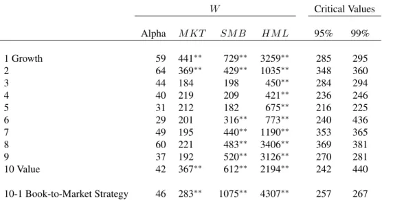
We now characterize the time variation of conditional betas from the one-factor market model. We begin by testing for constant conditional alphas and betas using the Wald test of Theorem 3. Table 3 shows that for all book-to-market portfolios, we fail to reject the hypothesis that the conditional alphas are constant, with Wald statistics that are far below the 95% critical values. This does not mean that the conditional alphas are equal to zero, as we estimate a highly significant long-run alpha of the book-to-market strategy and reject that the long-run alphas are jointly equal to zero across book-to-market portfolios. In contrast, we reject the null that the conditional betas are constant with p-values that are effectively zero.
Table 3:
Tests of constant conditional alphas and betas of book-to-market portfolios
Notes. We test for constancy of the conditional alphas and betas in a conditional capital asset pricing model using the Wald test of Theorem 3. In the columns labeled “Alpha” (“Beta”) we test the null that the conditional alphas (betas) are constant. We report the test statisticW in Theorem 3 and 95% and 99% critical values of the asymptotic distribution. We mark rejections at the 99% level with∗∗.
W Critical values
Portfolio Alpha Beta 95% 99%
1 Growth 49 424∗∗ 129 136 2 9 331∗∗ 65 71 3 26 425∗∗ 172 180 4 47 426∗∗ 202 211 5 30 585∗∗ 159 167 6 50 610∗∗ 276 286 7 75 678∗∗ 311 322 8 70 756∗∗ 276 286 9 84 949∗∗ 361 373 10 Value 116 1028∗∗ 320 331 10-1 Book-to-Market Strategy 114 830∗∗ 270 280
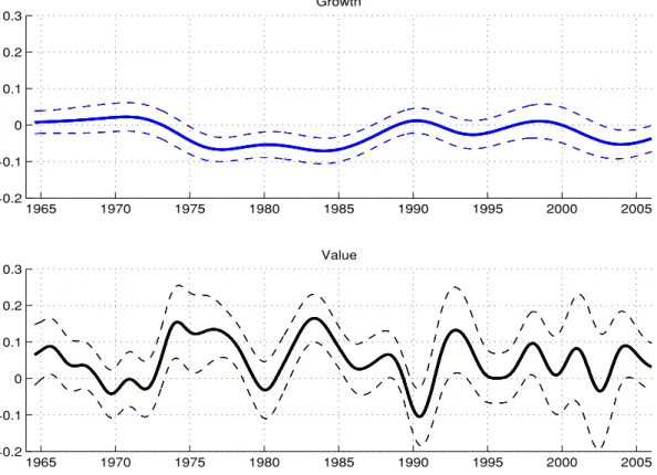
Fig. 2 charts the annualized estimates of conditional betas for the growth (decile 1) and value (decile 10) portfolios at a monthly frequency. Conditional factor loadings are estimated relatively precisely with tight 95% confidence bands, shown in dashed lines. Growth betas are largely constant around 1.2, except after 2000, when growth betas decline to around one. In contrast, conditional betas of value stocks are much more variable, ranging from close to 1.3 in 1965 and around 0.45 in 2000. From this low, value stock betas increase to around 1 at the end
of the sample. We attribute the low relative returns of value stocks in the late 1990s to the low betas of value stocks at this time.
Figure 2:
Conditional betas of growth and value portfolios
Notes. The figure shows monthly estimates of conditional conditional betas from a conditional capital asset pricing model of the first and tenth decile book-to-market portfolios (growth and value, respectively). We plot 95% confidence bands in dashed lines. The conditional alphas are annualized by multiplying by 252.
1965 1970 1975 1980 1985 1990 1995 2000 2005 0.4 0.6 0.8 1 1.2 1.4 Growth 1 1 7 1 7 1 1 1 1 2 2 0.4 0.6 0.8 1 1.2 1.4 Value
In Fig. 3, we plot betas of the book-to-market strategy, which is the difference in returns between deciles 10 and 1 (value minus growth). Because the conditional betas of growth stocks are fairly flat, almost all of the time variation of the conditional betas of the book-to-market strategy is driven by the conditional betas of the decile 10 value stocks. Fig. 3 also overlays estimates of conditional betas from a backward-looking, flat 12-month filter. Similar filters are employed by Andersen, Bollerslev, Diebold and Wu (2006) and Lewellen and Nagel (2006). Not surprisingly, the 12-month uniform filter produces estimates with larger conditional varia-tion. Some of this conditional variation is smoothed away by using the longer bandwidths of
our optimal estimators.9 However, the unconditional variation over the whole sample of the
uniform filter estimates and the optimal estimates are similar. For example, the standard de-viation of end-of-month conditional beta estimates from the uniform filter is 0.276, compared with 0.206 for the optimal two-sided conditional beta estimates. This implies that the Lewellen and Nagel (2006) analysis using backward-looking uniform filters is conservative. Using our optimal estimators reduces the overall volatility of the conditional betas, making it even more unlikely that the value premium can be explained by time-varying market factor loadings. Figure 3:
Conditional betas of the book-to-market strategy
Notes. The figure shows monthly estimates of conditional conditional betas of the book-to-market strategy. We plot the optimal estimates in bold solid lines along with 95% confidence bands in regular solid lines. We also overlay the backward one-year uniform estimates in dashed lines. National Bureau of Economic Research designated recession periods are shaded in horizontal bars.
1 1 7 1 7 1 1 1 1 2 2 −1 −0.5 0 0.5 Conditional Betas Backward Uniform Optimal
Several authors such as Jagannathan and Wang (1996) and Lettau and Ludvigson (2001b) 9The standard error bands of the uniform filters (not shown) are much larger than the standard error bands of the optimal estimates.