Attribute Selection Method based on Objective Data and Subjective Preferences in MCDM

Attribute Selection Method based on Objective Data

and Subjective Preferences in MCDM

X. Ma, Y. Feng, Y. Qu, Y. Yu Xiaofei Ma, Yi Feng

Technology Planning

Dalian Commodity Exchange Dalian City, China, 116023

[email protected], [email protected] Yi Qu*, Yang Yu

Agricultural Bank of China Data Center 88 Aoni Road, Pudong New Area Shanghai City, China, 200131

*Corresponding author: [email protected] [email protected]

Abstract: Decision attributes are important parameters when choosing an alter-native in a multiple criteria decision-making (MCDM) problem. In order to select the optimal set of decision attributes, an analysis framework is proposed to illustrate the attribute selection problem. Then a two-step attribute selection procedure is presented based on the framework: In the first step, attributes are filtered by using correlation algorithm. In the second step, a multi-objective optimization model is constructed to screen attributes from the results of the first step. Finally, a case study is given to illustrate and verify this method. The advantage of this method is that both external attribute data and subjective decision preferences are utilized in a sequential procedure. It enhances the reliability of decision attributes and matches the actual decision-making scenarios better.

Keywords: attribute selection, criteria decision-making (MCDM), multi-objective optimization, attribute correlation.

1

Introduction

Multi-criteria decision-making (MCDM) is successfully applied to help decision makers (DMs) choose optimal alternatives. During the past few decades, various MCDM methods have been proposed based upon different philosophies such as multi-attribute utility, the analytic hierar-chy process (AHP), outranking methods and so on. Meanwhile, many decision support systems (DSSs) have been designed in MCDM to assist DMs in analyzing problems and making decisions more easily. MCDM deals with a general class of problems that contains multiple attributes, objectives and criteria [20]; and alternatives are determined based on many qualitative or quan-titative criteria which are generally complicated and assessed by more relevant attributes. How-ever, not all of them can be used in decision-making procedure, because they contain plenty of redundant or "noisy" attributes and it will lead to useless decision alternatives. Therefore, the effectiveness of an alternative is highly dependent on the set of decision attributes.

The concept of "optimal" can be illustrated by two aspects: (1) Elements of the set are highly related to the MCDM problem for decision purpose; (2) The set of attributes is parsimonious, and the selected alternative will be suboptimum if one of these attributes is omitted. The rationale of attribute selection is similar to feature selection in data mining field. There are a lot of feature selection methods have been proposed, but only a few of them can be applied in decision-making process directly which are mentioned in the Literature Review part. Most of these methods can’t Copyright ©2018 CC BY-NC

account for both objective and subjective perspectives, so there is a low reliability of decision attributes. This study is focused on how to select the optimal set of decision attributes for a MCDM problem, external attribute data and subjective decision preferences are utilized in a sequential procedure to enhance the reliability of decision attributes.

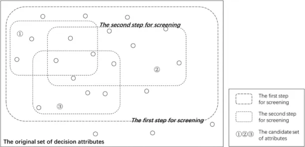
The attribute selection method for decision problem should account for both objective and subjective perspectives, more precisely, this paper merges attribute data (objective) with DMs’ requirement (subjective). Utilize the former for rational, constrained modeling and the latter for adapting specific problem issues to the decision-making process. In order to obtain the optimal set of attributes, an analysis framework for attribute selection problem and a two-step screening procedure is conducted in this paper. The specific procedure is illustrated in Figure 1.

Figure 1: The illustration for the presented method

This new attribute selection method in MCDM contributes to selecting the optimal set of decision attributes and helping DMs choose optimal alternatives better. Meanwhile, this method merges objective data and subjective preferences to improve performance for actual decision scenarios.

2

Literature review

Many feature selection methods have been proposed, and they are usually classified into three classes: "filter" methods, "wrapper" methods and "embedded" methods [2,7,8,14]. Wu [19] pro-posed using the fuzzy and grey Delphi methods to identify a set of reliable attributes and, based on these attributes, transforming big data to a manageable scale to consider their impacts. Meinshausen et al. [11] demonstrated linear model and Gaussian model of variable selection consistency in higher dimensional case. Although they have good performance, they cannot be applied in decision-making process directly (partial principle may be accepted). Only a few papers mentioned attribute selection in decision-making problems; for instance, Chun [4] con-sidered the "optimizing" and "satisficing" (a portmanteau of satisfy and suffice) attributes and deal with the multi-attribute decision problem with sequentially presented decision alternatives; Dai et al. [6] constructed three attribute selection approaches in context of incomplete deci-sion systems based on information-theoretical measurement of attribute importance; in order to screen the critical factors influencing the stability of perilous rock, Meng et al. [12] used fuzzy compromise TOPSIS method to calculate the importance of attributes in the decision problem.

Wu [18] used Fuzzy Delphi method to screen out the unnecessary attributes to deal with the complex interrelationships among the aspects and attributes. Attribute selection procedure can improve the decision performance, but no papers used this procedure in MCDM problems.

3

Method

3.1 Preliminaries

Trapezoidal fuzzy numbers

Definition 1. LetX be a universe set. Afuzzy _eain a universe of discourse X is characterized

by a membership function µ

e

a(x), which associates with each element x in X, a real number in the interval [0,1]. The function is termed the grade of membership of x in ea.

Definition 2. A tupleAe= (a, b, c, d), a≤b≤c≤d, is called a trapezoidal fuzzy number (TFN)

if its membership function is

µ e a(x) =        (x−a)/(b−a) a≤x≤b 1 b≤x≤c (d−x)/(d−c) c≤x≤d 0 otherwise

Wherea, b, c, d are real numbers.

Definition 3. Given two trapezoidal fuzzy numbersAe= (a₁, b₁, c₁, d₁),Ae= (a₂, b₂, c₂, d₂), and

a real numberλ, the main operations can be expressed as follows: 1 ○Af₁ L f A2= (a1+a2, b1+b2, c1+c2, d1+d2) 2 ○Af₁ N f A2= (a1a2, b1b2, c1c2, d1d2) 3 ○λN f A2 = (λa1, λb1, λc1, λd1) Multi-objective optimization

Let χ be a vector containing n decision variables and in a universe of discourse X.

Mathe-matically, an optimization problem with p objective functions can be expressed as (Mahdi and Seyed, 2012):

minimize fi(x) fori= 1,2, ..., p subject to: gj(x)≤0, j= 1,2, ..., q,

hj(x) = 0, j =q+ 1,2, ..., m

wherex= (x1, x2, ..., xn),xlis thelth decision variable;pandm are respectively the numbers of objective function and constraint.

A variety of methods can be used to solve this problem. One popular method is to combine those objectives into a single composite objective so that traditional mathematical programming methods can be applied. And other approaches are based on the Pareto optimum concept, and more specifically, let y= (y1, y2, ..., yn)be another vector containing n decision variables inX. Definition 4. (Domination) x ∈X dominates y ∈ X, denotedx y, if ∀j ∈ p,vj(x)≤vj(y) with at least one strict inequality.

Definition 5. (Pareto Optimal) xis a Pareto Optimal (PO) solution, if there is noy∈X such thatyx. The set of all Pareto optimal solutions in X is denoted PO(X).

These methods include Multiple Objective Genetic Algorithm (MOGA), Non-dominated Sorting Genetic Algorithm (NSGA), NSGA-II, Multi-objective Multi-state Genetic Algorithm (MOMS-GA), Niched-Pareto Genetic Algorithm (NPGA) and Multi-objective Particle Swarm Optimization (MOPSO) [9,21].

An analysis framework of attribute selection under MCDM

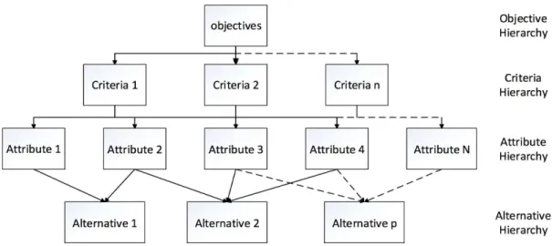
Multi-Criteria Decision Making (MCDM) has been widely applied as a well-known branch of decision making, and can be further divided into multi-objective decision making (MADM) and multi-attribute decision making (MODM) [5, 13]. The whole hierarchical structure of a MCDM problem is shown in Figure 2, and it can be unfolded from four hierarchies from top to the bottom, namely, objective, criteria, attribute and alternative.

(1) Objective Hierarchy: Generally contain multiple decision objectives given by DMs which reflect different decision requirement.

(2) Criteria Hierarchy: Criteria Hierarchy is to realize a fair comparison of alternatives from the various aspects of Objective Hierarchy, and it is also developed in a hierarchical fashion, starting from some general but imprecise criteria description, which is refined into more precise sub- and sub-sub criteria.

(3) Attribute Hierarchy: Attribute Hierarchy is determined by criteria Hierarchy and Objective Hierarchy. It is generally assumed that each criterion can be represented by some measur-able attributes of the consequences arising from implementation of any particular decision alternative [16], as well as objective. No matter what kind of MCDM methods, decision attributes are the bottom and direct evaluative parameters to determine alternatives. (4) Alternative Hierarchy: Consist from candidate alternatives evaluated by the set of decision

attribute.

Figure 2: The hierarchical structure of a MCDM problem

This paper focus on how to obtain the optimal set of decision attributes from Attribute Hierarchy for evaluating alternatives.

Rationale of the proposed method

Let O={O1_{, O}2_{, ..., O}γ_{} be a finite set of objectives, andC ={C}

1, C2, ..., Cn}be the set of

criteria. In most actual cases, objectives and criteria are always predetermined by MDs according to different knowledge background and decision experiences, thus we assume that all of objectives and criteria (or sub-criteria) are given.

We define decision attribute selection procedure as a sequential selection procedure based on objective and subjective information. It means that a series of screening steps will be applied in sequence to obtain an optimal set of attributes. A sequential screening can be described as follows [3]:

Scrh,h−1,...,1(Aoriginal) =Scrh(Scrh−1(...(Scr1(Aoriginal))...)) (1) where Scrk, k = 1,2, ..., h are screening steps, and Scrh is the final screening step in this sequential screening;Aoriginal={aj|j∈N} is the original set of decision attributes.

And two screening steps are conducted in proposed selection procedure, namely, Scr2,1(A) =

Scr2(Scr1(A)).

Scri is a screening step based on real-time attribute data, and the corresponding screening algorithm is established in the step. The result Scri(A)is to obtain a relatively optimized set of decision attributes AScr1 by deleting redundant attributes.

Scr2 is a further screening step based on the results of Scr2(A) to acquire the absolutely

optimal set of decision attributesAScr2. Decision goals that represent subjective preference are

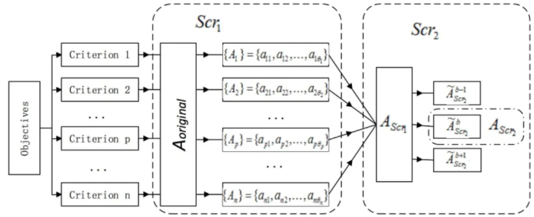
utilized in this step, and the selected set should satisfy all decision goals. The whole procedure of attribute selection is shown by Figure 3

Figure 3: The procedure of the proposed method whereAScr1 ={{A1},{A1}, ...,{Ap}, ...,{An}}, and Ae

b

Scr2 is candidate optimal set ofScr2.

3.2 A new method for attribute selection

Preprocessing of the data

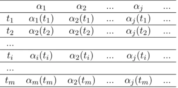
We consider three data types of decision attributes in this paper, namely, real numbers expressed asα0_{, intervals expressed as [α}L_{, α}U_{]and linguistic term set expressed as a linguistic} term setS={s0, s1, ..., sK}. And real-time attribute data can be listed as attribute value series

in Table 1.

Table 1: Attribute value series α1 α2 ... αj ... t1 α1(t1) α2(t1) ... αj(t1) ...

t2 α2(t2) α2(t2) ... αj(t2) ...

...

ti αi(ti) α2(ti) ... αj(ti) ...

...

tm αm(tm) α2(tm) ... αj(tm) ...

Both Scr1 and Scr2 are quantification procedures and therefore, in order to guarantee the

scientificity and preciseness of the presented method, preprocessing of attribute data need to be carried out firstly (referring to our previous work [10]).

(1) Convert attribute values to TFNs

For a real number α0_{, it can be denoted as a TFN (α}1_{, α}2_{, α}3_{, α}4_{), where α}1 _{= α}2 ₌

α3 _{= α}4 _{= α}0_{; for internal value bα}L_{, α}U_{c, the corresponding TFN can also be expressed} as (α1_{, α}2_{, α}3_{, α}4_{), where α}1 _{= α}2 _{= α}L _{and α}3 _{= α}4 _{= α}U_{. It is a little complex for a} linguistic term set with odd cardinalityS={s0, s1, ..., sK}, and the elementsK is converted

to the corresponding TFN as follows: (α1_k, α2_k, α3_k, α4_k) =    max 2k−1 2K+ 1,0 , 2k 2K+ 1, 2k+ 1 2K+ 1,min 2k+ 2 2K+ 1,1     (2) wherek= 0,1, ..., K.

(2) Normalize values of attributes

In real-world decision scenarios, some decision attributes are cost ones, which mean the lower the values of attributes, the better they will be; the others are benefit ones, which mean the higher the values of attributes, the better they will be. Without loss of generality, we assume that the attribute values can be expressed as αj(ti) = (α1j(ti), α2j(ti), α3j(ti), α4j(ti)), and normalized attribute values can be denoted asγj(ti) = (r1

j(ti), rj2(ti), rj3(ti), rj4(ti)). The normalized methods are given as follows:

• For cost attributes: rv_j(ti) = max i α4 j(ti) −αv j(ti) max i α4 j(ti) −min i α1 j(ti) v= 1,2,3,4. (3)

• For benefit attributes: rv_j(ti) = αv j(ti)−min i α1 j(ti) max i α4 j(ti) −min i α1 j(ti) v= 1,2,3,4. (4)

And the normalized attribute value series can be denoted as γ1 ={r1(t1), r1(t2), ..., r1(tm)};

γ2 ={r2(t1), r2(t2), ..., r2(tm)};

...;

γj ={rj(t1), rj(t2), ..., rj(tm)};

....

The first step for screening Scr1

In Scr1, one "relatively best" representative attribute will be chosen by DMs for each

crite-rion. It means that,

For ∀Cp ∈ {C1, C2, ..., Cn},1≤p≤n,

∃ap1∈Aoriginal, st.Cp ⇔ap1.

For example, "Economic losses" is a criterion in emergency decision, and "Amount of loss" is the "relatively best" attribute to evaluate loss degree. Thus the set {ap1|1 ≤ p ≤ n} is a

significant by-product after criteria determination, and actually it is the input ofScr1.

Scr1 is used to screen decision-relevant attributes from Aoriginal by analyzing attribute in-terrelation. More precisely, we will investigate geometrical relationship between attributes based on attribute value series; select highly correlative attributes forap1 fromAoriginal to constitute a

"relatively best" representative set for each criterionCi, and omit the rest of decision-irrelevant attributes. The step is entirely implemented on attribute value series without subjective impacts, and the outcomeAScr1 is a smaller and relative optimal set which the elements are determined

by evaluation criteria.

The idea of Scr1 arises from Grey Relational Analysis (GRA) Theory which provides a valid

way to quantify the interrelation of different factors using geometric methods [22]. And the detailed process of Scr1 is given in the following.

Step 1.1: Normalize attribute value series

It is different from normalization of attribute values, and it guarantees comparability of different attribute value series. The specific process is

yj ={aj(ti)/Dj, i= 1,2, ..., m} (5) Dj = 1 m−1 m X i=2 |aj(ti)−aj(ti−1)| (6)

whereyj is normalized attribute value series, andDj is increment average of yj.

Step 1.2: Calculate increment series

∆yj ={∆yj(ti) =yj(ti)−yj(ti−1), i= 2,3, ..., m} (7)

Step 1.3: Calculate correlation coefficient

AScr1 is obtained based on the input set{ap1|1≤p≤n} and thus, Step 1.3 will be stepwise

conducted for each elementap1. The correlation coefficient of differentti betweenap1 andaj can be defined as follows:

ξ(ti) = (

sgn(∆yp1(ti)·∆yj(ti))· min(

|∆yp1(ti)|,|∆yj(ti)|)

max(|∆yp1(ti)|,|∆yj(ti)|); j6=p1

0 ∆yp1(ti)·∆yj(ti) = 0

(8) where sgn(·) is a sign function; and sgn(∆yp1(ti) ·∆yj(ti)) = 1, if ∆yp1(ti) ·∆yj(ti) >

0;sgn(∆yp1(ti)·∆yj(ti)) =−1, if ∆yp1(ti)·∆yj(ti)<0.

Step 1.4: Calculate correlation degrees

τ(ap1, aj) = 1 d−c m X i=2 ∆ti·ξ(ti) (9) The correlation degrees reflect the closeness of two attributes; the greater the value of τ(ap1, aj) is, the closer the two attributes are, and the better the capability of aj is to

eval-uate criterionCp.

Step 1.5: Set threshold and screen correlation attributes for ap1

For∀Cp, a threshold of correlation degreeτ∗ should be set by DMs, and the attributeaj will be reserved, ifτ(ap1, aj)> τ∗. And the reserved attributes for evaluating Cp can be denoted as

{Ap}={ap1, ap2, ..., apθp}, where θp is the sum of attributes. In addition, the correlation degree

τ(ap1, apqp) betweenap1 and apqp will be abbreviated as zpqp, where1≤qp ≤θp. Step 1.6: Acquire the screening result set AScr1

Repeat Step 1.1 to Step 1.5 for each ap1, where 1≤p ≤n; and the result set AScr1 can be

obtained, namely,

AScr1 ={{A1},{An}, ...,{An}}.

The second step based on multi-objective optimization Scr2

Implementing decision attribute selection is aimed to assist DMs in evaluating alternatives for given decision problems and therefore, the selected attributes should be sensitive to the decision problem as well as familiar to DMs. Sensitivity reflects whether the selected attributes are accurate enough to represent the decision problem, and familiarity is used to estimate whether DMs are certain enough to make decision based on the selected attributes. For example, "fire duration" and "indoor fire load" are more important (sensitive) attributes than "carbon monoxide concentration" for evaluating fire grades; while it is more reliable for medical staff to estimate the physical condition of the wounded with "carbon monoxide concentration" than "Radiative Heat Flux".

Multi-objective optimization theory is a feasible way to quantify and synthesize these re-quirements, and it has solved similar problems in other areas successfully [1]. Thus three main objectives will be considered in this paper: attribute amount, attribute utility and attribute familiarity. Attribute amount should be as few as possible without reducing the validity of al-ternative, and it is the demand of bothScr2 and attribute selection method. Attribute utility is

used to distinguish attribute sensitivity in estimating the same decision problem, and attribute familiarity explores DMs’ cognition differences for decision attributes. The outcomeAScr2 drawn

from Scr2 should satisfy mentioned three goals, and now the optimal set of decision attributes

have been found afterScr1 and Scr2, namely, AScr2 =Scr2(Scr1(Aoriginal)).

A set of zero-one binary vectors{vb_{}withT = (θ}

1+θ2+...+θn)dimensionality will be defined

to represent different candidate outcome setAeb_Scr

1, where one represents the attribute belonging

to the set, otherwise it is zero. The optimal set of decision attributes is AScr2 ∈ {Aeb_Scr

1|b∈N},

and {Aeb_Scr

1}contains all the subsets of AScr1.

Three objective functions are defined firstly, and we will show that all the objective functions can be expressed as the functions with independent variablevb_.

Defining objective functions (1) Attribute utility function Attribute utility function measures decision sensitivity of Aeb_Scr

1, and it can be defined as

follows: U(Aeb_Scr 1) =g(M U(Ae b Scr1), W(Ae b Scr1)) (10)

where

1

○ M U(Aeb_Scr

1) =v

b_{·M U}∗ ₍₁₁₎

M U∗ represents attribute utility matrix, and it is diagonal matrix with the diagonal elements

∆a11 ∆a11, ..., ∆a11 ∆a1θ1, ..., ∆ap1 ∆apqp, ..., ∆an1 ∆an1, ..., ∆an1 ∆anθn.

More precisely, M U∗ can be explained by a marginal utility function u(·), namely, u(apqp) =

∆ap1

∆apqp

1≤p≤n,1≤qp ≤θp; (12) where ∆ap1 is increment of ap1, and ∆apqp is the corresponding varying of apqp. And the

functionu(·)quantifies the assessment performance on criterionCi of the attributeapqp according

to calculate the ratio between increments of the two attribute values.

In fact, M U∗ can be predetermined by domain experts, because plenty of field studies have been conducted to investigate utility relation of attributes.

2

○W(Aeb_Scr

1) =W

∗_·(vb₎0 ₍₁₃₎

W∗ represents attribute weighting matrix, and it is also a diagonal matrix with diagonal elements w11, ..., w1θ1, ..., wpqp, ..., wn1, ..., wnθn.

where

wpqp =ωp·zpqp, 1≤p≤n,1≤qp ≤θp; (14)

and {ω1, ω2, ..., ωn}are the know weights of C={C1, C2, ..., Cn}.

g(·)is a dot product function and therefore, U(Aeb_Scr

1) can be transformed into the following

function with independent variablevb_{, namely,}

U(vb) = (vb·M U∗)·(W∗·(vb)0) (15) (2) Attribute familiarity function

Attribute familiarity function is established to quantify DMs’ cognition degrees on different candidate set Aeb_Scr

1, and it is defined as

F(vb) =η·σ·(vb)0 (16) In Eq. 16, η = (η1, η2, ..., ηL)1×L is the weight vector of DMs, and L is the number of DMs; σ is attribute familiarity matrix with the following expression

σ=         σ1(1) σ2(1) ... σT(1) σ1(2) σ2(2) ... σT(2) · · · · · · · · · σ1(L) σ2(L) ... σT(L)         L×T (17)

and σh(l)represents thelth DM’s familiarity degree with attribute ah, where1≤l≤L, and 1≤h ≤T. Attribute familiarity is usually evaluated qualitatively by DMs, and many methods can be applied to quantify assessment results and obtain matrix σ, such as AHP and fuzzy set theory.

Attribute count function calculates the attribute number of a candidate setAeb_Scr

1, and it can

be defined by means of vector length formula, Count(Aeb_Scr

1) =|v

b_|2 ₍₁₈₎

where|vb_{|represents the length of vectorv}b_.

Establish multi-objective optimization model for Scr2 After define relevant objective

functions, the multi-objective optimization model of Scr2 is established to obtain the Pareto

Optimal solutionsAScr2, as well as the optimal set of decision attribute selection problem.

M aximize U(vb_{) = (v}b_{·M U}∗_)·(W∗_·(vb₎0₎ F(vb_{) =η·σ·(v}b₎0 (19) M inimize Count(Aeb_Scr 1) =|v b_|2 Subject to: |vb|2 ≥n

The model Eq. 19 can be solved by aforementioned algorithm, such as MOGA, NSGA, MOMS-GA and traditional mathematical programming methods, and it depends the specific model drawn from given decision problems and decision requirements.

4

Empirical results

4.1 Accident scenario and computational settings

In order to validate the presented method, a fire accident scenario will be constructed and simulated. The fire happens in a factory dormitory, and two workers are asleep; some inflammable are stacked near the door which arise spontaneous combustion for some reasons. The total layout of this room is illustrated in Figure 4, containing three beds, two workers marked by fellow cuboids, fire origin and plenty of fire smoke. Now two experts need to make rescue alternative based on the collected data; one is fire expert who are engaged in fire research for many years and have in-depth study of the fire attributes, and the other is an experienced firefighter who know some medical knowledge. And they are weighted with0.6and0.4respectively. A fire simulation software FDS [17] is used to establish fire scenario and generate fire data.

The purpose of simulation is not only to provide a fire scenario, and more importantly, it can generate relevant fire attributes data for the following experiment. The data can be exported from FDS containing attribute names, physical dimensions, attribute values and attribute types. In this paper, we generate twelve fire attributes and 125 data records.

4.2 Select fire attributes by utilizing the presented method

In this fire scenario, three main criteria will be considered, i.e., fire behavior, personal security and environmental conditions, and corresponding attributes are shown in Table 5

where "Enthalpy" is an interval attribute, "Indoor fire load" and "Circuit aging degree" are linguistic attributes, and the rest are real number attributes. The bold attributes are "relatively best" representative attributes for each criterion.

Figure 4: A simulated fire scenario

Table 2: List of criteria and corresponding attributes

Criterion Attributes

Fire behavior Temperature / Enthalpy / Heat Release Rate / Relative Humidity / Burning Rate / Pressure / Radiative Heat Flux Personal security Carbon monoxide/ Carbon dioxide / oxygen

Environmental conditions Indoor fire load/ Circuit aging degree

As aforementioned, the real number attributes and interval attributes can be denoted by TFNs directly. The linguistic attributes "Flammable of storage items" and "Circuit aging degree" can be transformed into TFNs in Table 3.

Table 3: Linguistic attributes and corresponding TFNs Linguistic terms TFNs Not dangerous (0,0,0.111,0.222) Medium dangerous (0.111,0.222,0.333,0.444) Dangerous (0.333,0.444,0.555,0.666) Very dangerous (0.555,0.666,0.777,0.888) Highly dangerous (0.777,0.888,0.999,1)

Then we carry out normalization by Eq. 3 and Eq. 4 to obtain corresponding TFNs.

(2) The first step for screening Scr1

Without loss of generality, the criterion "Fire behavior" will be utilized to illustrate the first screening procedure and the other two criteria "Personal security" and "Environmental conditions" can be dealt with similarly.

The criterion "Fire behavior" is represented by seven attributes, namely, "Temperature", "Enthalpy", "Heat Release Rate", "Relative Humidity", "Burning Rate", "Pressure" and "Ra-diative Heat Flux"; and "Temperature" is the "relatively best" representative attribute for the criterion "Fire" behavior.

Step 1.1 to Step 1.4 are implemented to calculate correlation degrees between

""Tempera-ture" and the remaining six attributes, and the results are given in Table 4.

Table 4: Correlation degrees between "Temperature" and the other six attributes Attribute Enthalpy Heat Release

Rate RelativeHumidity BurningRate Pressure RadiativeHeat Flux Correlation degree 0.53745 0.96987 0.33271 0.74787 0.47665 0.88712

Step 1.5: Set threshold of correlation degree τ∗ = 0.6

Thus the attributes will be reserved whose correlation degrees is greater than or equal to 0.6, i.e., "Burning Rate", "Heat Release Rate" and "Radiative Heat Flux".

Step 1.6: Repeat Step 1.1 to Step 1.5 for each criterion

For criteria "Personal security" and "Environmental conditions", the "relatively best" rep-resentative attributes are respectively "Carbon monoxide" and "Indoor fire load", and relevant correlation degrees are shown in Table 5.

Table 5: Relevant correlation degrees for the other two criteria Criterion Personal security Environmental conditions Attribute Carbon dioxide oxygen Circuit aging degree Correlation degree 0.80961 0.93428 0.76865

We reset thresholds of correlation degree for each criteria, viz.,τ∗

P ersonal= 0.9andτEnvironmental∗ = 0.8.

Finally, the result of the first screening AScr1 can be obtained, namely,

AScr1 = {"Temperature", "Heat Release Rate", "Radiative Heat Flux", "Burning Rate",

"Carbon monoxide", "oxygen", "Indoor fire load"}.

(3) The second step for screening Scr2

Before conducting Scr2,M U∗,σ and W∗ should be given firstly. As aforementioned, M U∗

andσcan be determined by relevant research achievements and expert experiences, and therefore, we collected and integrated evaluation results from ten fire researchers to assign M U∗ andσ as follows: M U∗ =           19.5 15.6 7.4 11.2 15.4 18.7 18.2           and σ= 9 8 8 9 4 4 5 4 5 4 4 9 9 7

where the elements values of M U∗ are in the interval [0, 20], and the greater the value is, the more sensitive the attribute is for evaluation. The elements values ofσ are in the interval [0, 10], and the greater the value is, the more familiar the attribute is to DMs.

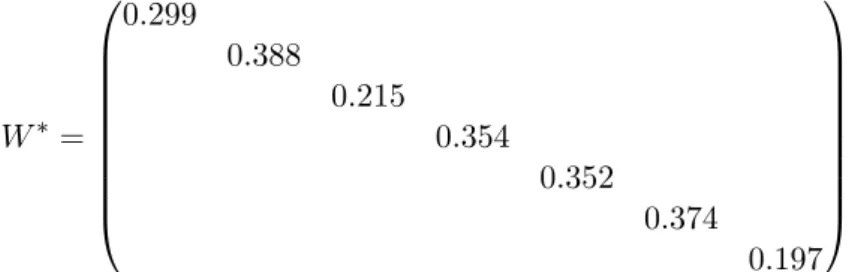
Moreover,W∗can be acquired with the given criteria weight vector(ω1, ω2, ω3) = (0.4,0.4,0.2), namely, W∗ =           0.299 0.388 0.215 0.354 0.352 0.374 0.197          

After determine relevant parameters M U∗, W∗, σ, and the seven-dimensional independent variablevb_,Scr

2 based on the multi-objective optimization model Eq 19 is performed in Matlab

R2013b. We choose the traditional mathematical programming method to solve this model, because the research [15] has proven that the programming method has better performance than aforementioned other algorithms to solve such a problem with the zero-one binary vector variable and the small size of data.

The results are shown in Figure 5 where the curve represents all possible solutions and the Pareto Optimal solution is the intersection of the curve and the x-axis, namely, vb ₌ (1,1,0,1,1,1,1). It means that the attribute "Radiative Heat Flux" represented by zero can be omitted, and the optimal set of decision attributes is:

AScr2 = {"Temperature", "Heat Release Rate", "Burning Rate", "Carbon monoxide",

"oxy-gen", "Indoor fire load"}.

Figure 5: The results of the second step Scr2

4.3 Validation of the presented method

In order to verify the result is the optimal set for a MCDM problem, multi-attribute utility theory will be used in the following.

A conclusion underlies the presented method: Removing decision-irrelevant attributes from the set of decision attributes will improve the effectiveness of decision alternatives. Thus it is reasonable and feasible to verify our work starting fromScr2, because the purpose of Scr1 is to

Multi-attribute utility theory (MAUT) is used to choose decision alternatives by evaluating the utility values of alternatives which is calculated based on the utility of decision attributes, and it is an effective way to quantify decision attributes’ impact on decision results. More precisely, the utility evaluation model of an alternative is given as follows:

u(x1, x2, ..., xn) = n X i=1 kiui(xi) if n X i=1 ki = 1 (20)

where xi is the ith decision attribute, and ki is the corresponding weight; ui(xi) is the at-tribute utility function ofxi, andu(x1, x2, ..., xn)is the utility function of an alternative evaluated by x1, x2, ..., xn.

Thus the utility values of all possible candidate sets Aeb_Scr

1 are calculated based on Eq. 20,

where attribute utility function ui(xi) can be defined as Eq. 12, and the weights are acquired by Eq. 14. It should be pointed that normalization of weights need be carried out to guarantee

n P i=1

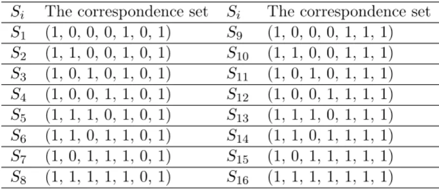
ki= 1. And the results are given in Table 6, whereSirepresents the candidate set of decision attributes, and 1≤i≤16. The correspondence between Si and the set of attributes are shown in Table 7.

Table 6: The utility values of attribute sets

Attribute set S1 S2 S3 S4 S5 S6 S7 S8

Utility value 23.621 24.343 28.496 28.923 29.665 31.745 28.474 29.500

Attribute set S9 S10 S11 S12 S13 S14 S15 S16

Utility value 25.908 28.447 32.631 31.229 30.335 35.774 31.658 33.439

Table 7: The correspondence betweenSi and the set of attributes Si The correspondence set Si The correspondence set S1 (1, 0, 0, 0, 1, 0, 1) S9 (1, 0, 0, 0, 1, 1, 1) S2 (1, 1, 0, 0, 1, 0, 1) S10 (1, 1, 0, 0, 1, 1, 1) S3 (1, 0, 1, 0, 1, 0, 1) S11 (1, 0, 1, 0, 1, 1, 1) S4 (1, 0, 0, 1, 1, 0, 1) S12 (1, 0, 0, 1, 1, 1, 1) S5 (1, 1, 1, 0, 1, 0, 1) S13 (1, 1, 1, 0, 1, 1, 1) S6 (1, 1, 0, 1, 1, 0, 1) S14 (1, 1, 0, 1, 1, 1, 1) S7 (1, 0, 1, 1, 1, 0, 1) S15 (1, 0, 1, 1, 1, 1, 1) S8 (1, 1, 1, 1, 1, 0, 1) S16 (1, 1, 1, 1, 1, 1, 1)

In Table 6, for ∀i, 1 ≤ i ≤ 16, it has u(S14) > u(Si), where i 6= 14. The set S14 has

the maximum utility value u(S14) = 35.774, and thus the alternative chosen based on S14 (the

optimal setAScr2) is the optimal alternative.

In addition,S1 contains three attributes with minimum utility valueu(S1) = 23.621, andS16

attributes are not available in a MCDM problem; too few attributes are not enough to evaluate the decision problem, while too many attributes may lead to conflict and interfere decision results. The set of decision attributes obtained by utilizing the presented method has the maximum utility value in alternative evaluation, and it demonstrates the effectiveness of the presented method.

5

Implications

This paper utilizes attribute selection procedure in MCDM problems innovatively. MCDM problems refer to getting the optimal alternatives which are determined based on many quali-tative or quantiquali-tative criteria, and these criteria are conflicting and assessed by more relevant attributes. Therefore, the set of decision attributes determines the effectiveness of an alternative. In order to improve the reliability of MCDM, the method proposed in this study can select the optimal set of decision attributes which are highly related to the MCDM problem and remove redundant or "noisy" attributes. Meanwhile, the selection of optimal set can reduce the attribute dimension and improve the efficiency of decision making while maintaining the great effect.

The method combines external attribute data with subjective decision preferences in the sequential procedure to improve decision performance. External attribute data are objective factors, which show the features of the data. These attributes contain its own regularity and all kinds of information that decision-making needs, so the first step to screen is based on objective attribute data. Subjective factors show the decision makers’ preferences. Because of the different profession and background knowledge, decision makers have different recognition of attributes. Considering the subjective decision preferences contributes to improve the reliability and accuracy of decision-making. Using the former to build the method and using the constraint conditions of the latter to adjust the method can make it more in line with the actual situation. The method combines external attribute data with subjective decision preferences in the sequential procedure to improve decision performance. External attribute data are objective factors, which show the features of the data. These attributes contain its own regularity and all kinds of information that decision-making needs, so the first step to screen is based on objective attribute data. Subjective factors show the decision makers" preferences. Because of the different profession and background knowledge, decision makers have different recognition of attributes. Considering the subjective decision preferences contributes to improve the reliability and accuracy of decision-making. Using the former to build the method and using the constraint conditions of the latter to adjust the method can make it more in line with the actual situation.

6

Conclusions

In this paper, a new attribute selection method with the context of MCDM is proposed. According to the analysis of attribute selection problem, a two-step procedure is established to reduce original set to the optimal set of decision attributes. GRA theory and multi-objective optimization method are respectively used to implement these two screening steps. And then a fire example is shown to illustrate application and validity of screening method. The attribute selection method presented in this paper is a dynamic and flexible procedure which depends on decision data resource and decision requirement. It eliminates the drawback that decision at-tributes are chosen completely subjectively, and it will show better performance for new decision scenarios.

Attribute selection is also a critical process for many domains, such as classification problem, clustering problem, risk assessment, credit assessment, etc. And even solution of these issues

depended on results of attribute selection. Attribute selection problem is also discussed in data mining called "Feature Engineering", and still has needs to continue thorough research and the technique problem to be solved.

Generally it exists plenty of missing data among decision information, and how to select the optimal decision attributes in this case will be our future research.

Bibliography

[1] Babaei, S., Sepehri, M. M., Babaei, E. (2015). Multi-objective portfolio optimization consid-ering the dependence structure of asset returns. European Journal of Operational Research,

244(2), 525-539, 2015.

[2] Bermejo, P., Gamez, J. A., Puerta, J. M. (2014). Speeding up incremental wrapper feature subset selection with Naive Bayes classifier. Knowledge-Based Systems, 55, 140-147, 2014.

[3] Chen, Y., Kilgour, D. M., Hipel, K. W. (2008). Screening in multiple criteria decision analysis. Decision Support Systems, 45(2), 278-290, 2008.

[4] Chun, Y. H. (2015). Multi-attribute sequential decision problem with optimizing and satis-ficing attributes. European Journal of Operational Research, 243(1), 224-232, 2015.

[5] Comes, T., Hiete, M., Wijngaards, N., Schultmann, F. (2011). Decision maps: A framework for multi-criteria decision support under severe uncertainty.Decision Support Systems, 52(1),

108-118, 2011.

[6] Dai, J., Wang, W., Tian, H., Liu, L. (2013). Attribute selection based on a new conditional entropy for incomplete decision systems. Knowledge-Based Systems, 39, 207-213, 2013.

[7] Hapfelmeier, A., Ulm, K. (2014). Variable selection by Random Forests using data with missing values, Computational Statistics &Data Analysis, 80, 129-139, 2014.

[8] Huda, S., Abdollahian, M., Mammadov, M., Yearwood, J., Ahmed, S., Sultan, I. (2014): A hybrid wrapper-filter approach to detect the source (s) of out-of-control signals in multi-variate manufacturing process, European Journal of Operational Research, 237(3), 857-870,

2014.

[9] Lin, Q., Li, J., Du, Z., Chen, J., Ming, Z. (2015). A novel multi-objective particle swarm optimization with multiple search strategies, European Journal of Operational Research,

247(3), 732-744, 2015.

[10] Ma XF, Zhong QY, Qu Y (2013) Determination method of emergency key property based on common knowledge model and Euclidean distance, Systems Engineering, 31(10), 93-97,

2013.

[11] Meinshausen, N., Buhlmann, P. (2010): Stability selection.Journal of the Royal Statistical Society: Series B (Statistical Methodology), 72(4), 417-473, 2010.

[12] Meng MH, Pei XJ, Wu MQ (2015): Study on choice of factors influencing stability of perilous rock based on fuzzy multi-attribute group decision-making. Subgrade Engineering, 1:20-23,

2015.

[13] Montajabiha, M. (2016): An Extended PROMETHE II Multi-Criteria Group Decision Mak-ing Technique Based on Intuitionistic Fuzzy Logic for Sustainable Energy PlannMak-ing.Group Decision and Negotiation, 25(2), 221-244, 2016.

[14] Robin, G., Jean-Michel P., Christine T. (2010): Variable selection using random forests,

Pattern Recognition Letters, 31, 2225-2236, 2010.

[15] Shen HP, Zhang YP, Wang YK (2014): Research on regular Chinese fragments reassembly based on 0-1 programming model, Electronic Science and Technology, 6:13-16, 2014.

[16] Stewart, T. J. (1992): A critical survey on the status of multiple criteria decision making theory and practice, Omega, 20(5-6), 569-586, 1992.

[17] Wahlqvist, J., Van Hees, P. (2013): Validation of FDS for large-scale well-confined mechani-cally ventilated fire scenarios with emphasis on predicting ventilation system behavior,Fire Safety Journal, 62, 102-114, 2013.

[18] Wu, K. J., Tseng, M. L., Chiu, A. S., Lim, M. K. (2016): Achieving competitive advan-tage through supply chain agility under uncertainty: A novel multi-criteria decision-making structure, International Journal of Production Economics, article in press, 2016.

[19] Wu, K. J., Liao, C. J., Tseng, M. L., Lim, M. K., Hu, J., Tan, K. (2017): Toward sustainabil-ity: using big data to explore the decisive attributes of supply chain risks and uncertainties,

Journal of Cleaner Production, 142, 663-676, 2017.

[20] Zeleny, M., Cochrane, J. L. (1973): Multiple criteria decision making, University of South

Carolina Press, 1973.

[21] Zhang, Y., Gong, D., Cheng, J. (2017): Multi-Objective Particle Swarm Optimization Ap-proach for Cost-based Feature Selection in Classification,IEEe/ACM Transactions on Com-putational Biology and Bioinformatics, 14, 64-75, 2017.

[22] Zhu, J., Zhang, S., Chen, Y., Zhang, L. (2016): A hierarchical clustering approach based on three- dimensional gray relational analysis for clustering a large group of decision makers with double information, Group Decision and Negotiation, 25(2), 325-354, 2016.