Towards autonomous decision-making: A probabilistic model for learning multi-user preferences

(1)

Towards autonomous decision-making:

A probabilistic model for learning

multi-user preferences

Markus Peters and Wolfgang Ketter

May 2013

ERS-2013-007-LIS

Department of Decision and Information Sciences Rotterdam School of Management

Erasmus University

3062 PA Rotterdam, The Netherlands

Abstract

Information systems have revolutionized the provisioning of decision-relevant information, and decision support tools have improved human decisions in many domains. Autonomous decision-making, on the other hand, remains hampered by systems’ inability to faithfully capture human preferences. We present a computational preference model that learns unobtrusively from lim-ited data by pooling observations across like-minded users. Our model quantifies the certainty of its own predictions as input to autonomous decision-making tasks, and it infers probabilistic segments based on user choices in the process. We evaluate our model on real-world preference data collected on a commercial crowdsourcing platform, and we find that it outperforms both individual and population-level estimates in terms of predictive accuracy and the informative-ness of its certainty estimates. Our work takes an important step toward systems that act autonomously on their users’ behalf.

(2)

Keywords: Assistive technologies, Autonomous decision-making, Multi-task learning, Pref-erences, Software agents

(3)

1 Introduction

Enhancing individual and organizational performance through information technology is one of Information Systems’ (IS) fundamental promises – a promise on which the discipline has delivered in many important ways. Consumers can now choose among an unprecedented variety of affordable products and services online; and managers routinely make decisions based on rich, differentiated real-time information about their organizations and global markets, to name just two significant developments of recent years. But while information systems have become increasingly adept at provisioning relevant information and supporting human decision-makers, autonomous decision-making remains elusive under all but the most highly structured circumstances.

Dynamic flight pricing and automated credit approvals are two prominent examples of pro-cesses that have been successfully codified to the point where business rule engines are now making most operative decisions quickly, cheaply, and reliably [Davenport and Harris, 2005]. But in less clearly structured settings – from booking the next vacation to trading in complex multi-echelon markets – computer-assisted human decision-making remains the gold standard. Delegating decision-making to an autonomous software agent in these settings is often not so much hampered by the agent’s inability to select a good decision, as it is by an inability to

determine what constitutes a good decision in the user’s eyes to begin with. In many cases, the autonomous decision-making challenge amounts to a challenge in eliciting and faithfully representing human preferences using a computational model [Bichler et al., 2010].

To be useful, the preference model employed by an autonomous software agent must meet a broad range of requirements. Most importantly, it must respect the numerous systematic in-consistencies in human preferences that psychologists have discovered and carefully documented over the last decades [Slovic, 1995, Lichtenstein and Slovic, 2006]. The uncertainty that these inconsistencies give rise to are a crucial ingredient for autonomous decision-making: an agent should only make high-value decisions autonomously if past evidence suggests that its actions will be correct with high probability; otherwise, the agent should prompt its user for additional information. Allowing the threshold for user involvement to change over time is referred to as adjustable autonomy [Tambe et al., 2002]. Adjustable autonomy is an important determinant of users’ trust in autonomous agents, and a good preference model will provide estimates of its own uncertainty to facilitate it. Finally, autonomous agents cannot demand their user’s attention too frequently and the preference models they employ must therefore begin to make accurate predictions after observing limited training data. In an information systems setting, this means that a preference model should be (a) flexible enough to learn from multiple types of data (e.g., observed click streams and explicit critiques of alternatives by the user), and (b) pool data from like-minded users in a principled way [Ansari et al., 2000].

Our main contribution is MEP, a novel Mixed-Effect Preference model that meets these requirements. MEPis a semi-parametric Bayesian model that quantifies the uncertainty of its own predictions based on probabilistic principles. The Bayesian framework allows us to cleanly separate between evidence and inference and, as such, to integrate multiple types of preference information incrementally, an essential property in information system settings. The type of preference information that we focus on are pairwise comparisons of the form “User U prefers alternative A over B”, whereas much previous work has focussed on ratings [Adomavicius and Tuzhilin, 2005a].

While reasoning based on ratings is significantly easier, there are three important motiva-tions for studying pairwise comparisons: First, pairwise comparisons are more informative in the sense that they do not force users into self-consistency. Whereas rating systems suppress, e.g., intransitivity,MEPembraces inconsistencies and lets them unfold in the form of uncertain-ties. Second, pairwise choice situations are cognitively easier on users and evoke a qualitative reasoning mode in contrast to the quantitative reasoning evoked by ratings, making them an interesting subject of study in their own right [Slovic, 1995]. And third, pairwise choices are

(5)

often readily derived from users’ actions in information systems which reduces the user’s burden compared to providing explicit training information.

MEPfurther reduces users’ burden by systematically pooling observations across like-minded users, thus reducing the amount of information required from each individual. In the process, it discovers naturally occurring segments of users based on their choices. Regular segmenta-tion techniques proceed by first segmenting users heuristically (based on approximasegmenta-tions such as demographics, or heuristic global search) and then building a separate model for each seg-ment [Jiang and Tuzhilin, 2009], but user demographics and other statistics are inherently limited in their ability to truly reflect user preferences, e.g., [Reinecke and Bernstein, 2012]. In contrast, in MEPsegments are induced by choices which gives rise to a principled new approach to user segmentation. Importantly, inference in our model remains computationally within reach of deterministic approximations, whereas previous work had to resort to slower sampling methods, e.g., [Ansari et al., 2000].

We demonstrate the qualities ofMEPin experiments on a real-world dataset collected specifi-cally for this study. Earlier work has measured pairwise preference learning performance mostly on converted rating or regression datasets. But these tasks are fundamentally different from pairwise comparisons and the resulting datasets are unlikely to reflect human choice behavior well. We acquired our data through Amazon Mechanical Turk, a commercial crowdsourcing plat-form, a practice that is gradually becoming more popular in psychology and the social sciences, but that we have so far not encountered in preference learning. As such, our data collection methodology is an interesting contribution in its own right.

The work we present here is related to an earlier study [Peters and Ketter, 2012] that was in-spired by the same problem, but that used a more heuristic approach to preference modeling. In contrast, in this article we give a rigorous mathematical derivation of our mixed-effect preference model, complete with formal convergence guarantees. MEP now employs a fully probabilistic segmentation (“soft clustering”) whereas our previous work was limited to deterministic segment assignments.

The remainder of this article is structured as follows: In Section 2 we present related work in Computer Science, Econometrics, Information Systems, Marketing, and Psychology. MEP is introduced in Section 3 and experimentally evaluated in Section 4. We discuss our work, and conclude with directions for future research in Section 5.

2 Related Work

Human preferences have long been a subject of interest for scholars from a multitude of fields including Information Systems, Computer Science, Psychology, Marketing, and Econometrics. Much like our study is biased by our own Information Systems weltanschauung, these works have looked at human preferences from a diverse set of angles, from descriptive to normative. Before introducing our own preference model in Section 3, we first consider selected contributions made in each of these fields, and we discuss their relationship to our work. In the interest of space, we will not strive for comprehensiveness. Instead, the idea that we wish to convey is that preferences are too rich and faceted as a phenomenon to admit mono-disciplinary study; scholars from all aforementioned fields are now embracing this insight to develop models and theories that transcend the traditional boundaries of their disciplines.

2.1 Information Systems

Within IS, our work is most closely related to the literature onrecommender systems, which are concerned with finding and recommending items of interest, e.g., in electronic commerce set-tings [Adomavicius and Tuzhilin, 2005a]. Our work shares the design science perspective [Hevner et al., 2004] that is prominent in this literature in the sense that we aim to design an artifact (a

(6)

preference model), the ultimate purpose of which is to be useful; we also adopt several dimen-sions of usefulness that are important in recommender systems. Specifically, our model must be computationally tractable, suitable for operation within real-world information systems, predict preferred alternatives accurately, and be able to operate on limited input data. In other regards, the problem we study is different and in some sense harder than the recommendation problem: 1. Our model targets autonomous decision-making settings instead of giving recommenda-tions, a difference that is reflected in the probabilistic design of our model. Autonomous decisions are becoming increasingly important in fast-paced, data-intensive electronic mar-ketplaces [Peters et al., 2013] and we contend that these settings will require a principled quantification of uncertainty that allows software agents to return control to their users in cases of doubt. Some previous recommender systems studies make use of probabilistic models in focussed application areas (e.g., click-stream mining [Manavoglu et al., 2003]), but these works are not easily generalized to the autonomous decision-making task we consider.

2. Most recommender systems operate based onratings which have several drawbacks in the context of autonomous decision-making. We already pointed out that ratings force users into self-consistency, invoke quantitive reasoning patterns, and are potentially intrusive. Moreover, ratings provide a comparatively coarse image of user preferences, a problem that is acknowledged in the development of multi-criteria recommender systems [Manouselis and Costopoulou, 2007]. And finally, ratings are subjective in the sense that two decision-makers may share the same preferences but assign different ratings to alternatives [Jin et al., 2002].

A particularly interesting development in the recommender systems community is the increasing adoption of psychological notions like time variability, iterative refinement, or context depen-dencies [Palmisano et al., 2008, Adomavicius and Tuzhilin, 2011]. Our model contributes to this discussion through its ability to detect inconsistencies in preferences stated at different times or in different contexts.

Other related research includes work on personalization [Murthi and Sarkar, 2003, Adomavi-cius and Tuzhilin, 2005b] which studies methods for adapting products and services, often in digital environments where associated costs are low. For example, [Atahan and Sarkar, 2011] propose a Bayesian method for the accelerated learning of user profiles through dynamic adap-tion of navigaadap-tion opadap-tions. Several other IS scholars have worked on methods that span across multiple academic disciplines. For example, [Huang et al., 2012] propose a discrete choice pre-diction method based on Machine Learning techniques, and [Roy et al., 2008] combine ideas from Multi-Criteria Decision Analysis (MCDA) and Operations Research to learn utility func-tions. These works are related to ours in isolated aspects, but they generally follow different objectives; to our knowledge, our study is the first to combine probabilistic estimates, systematic data pooling across multiple users, flexibility with respect to different types of preference data, and a principled approach to segmentation in one coherent method.

2.2 Computer Science

Researchers in Artificial Intelligence (AI) have a long-standing interest in preferences as a flexible alternative to the notion of goals, reviewed in [Brafman and Domshlak, 2009]. It may not be clear from the outset whether a certain goalis attainable, but using apreference relation, an intelligent agent can work towards the most favorable outcome that is attainable under given circumstances. AI researchers realized the importance of preferences for autonomous decision-making agents early on [Maes, 1994, Brachman, 2002], and they proposed a series of innovative representations for preference relations and associated reasoning schemes, e.g., [Boutilier et al., 2004]. However, most of these representation are based on a markedly normative understanding

(7)

of human preferences. That is, they make strong rationality assumptions and reasoning conse-quently becomes difficult when they are confronted with actual human preferences, e.g., [Cheva-leyre et al., 2011].

Machine Learning (ML), on the other hand, takes a data-driven, predictive approach to preferences, and researchers in the field have proposed models based on a broad variety of learning techniques [F¨urnkranz and H¨ullermeier, 2011]. Of particular interest to us is work on probabilistic preference models that yield uncertainty estimates based on noisy preference observations. [Chu and Ghahramani, 2005b] were the first to model preference learning as a problem in probabilistic ordinal regression, and their work has spawned a series of innovative extensions that, for example, incorporate relational information [Kersting and Xu, 2009, Xu et al., 2010] or improve scalability [Nielsen et al., 2011]. What is absent from these studies, how-ever, is the ability to pool preferences across like-minded users to learn from limited information, or multi-task learning in ML terminology [Caruana, 1997]. [Bonilla et al., 2010] propose that multi-task preference learning can be realized by incorporating user information into preference statements, [Houlsby et al., 2012] propose a mixture of Gaussian processes model, and [Birlutiu et al., 2012] couple several single-user tasks through a hierarchical prior. But these approaches are either not applicable to our scenario (because user information may not be available), or they lack the segmentation based on stated preference that we aim for.

2.3 Psychology

Scholars in Psychology have primarily taken an explanatory interest in human preferences. One of the key achievements of the discipline has been the establishment of positive theories of human preferences [Tversky and Kahneman, 1992, Slovic, 1995, Thaler, 2000, Lichtenstein and Slovic, 2006] next to the normative theories from Economics [von Neumann et al., 2007]. These positive theories attest that human preferences are inconsistent, constructed as needed, and that the construction process depends on situational framing and environmental factors, among other influences. The probabilistic nature of our model acknowledges such inconsistencies and lets them unfold in the form of uncertainties. They are an important output of our model: an autonomous decision-making agent can use them to return control to its user when uncertain about a high-value decision.

2.4 Marketing and Econometrics

Finally, our work is related to the Marketing and Econometrics literature where preference measurement methods such as conjoint analysis, logit/probit models, and several other dis-crete choice prediction techniques [Greene, 2012] were pioneered. Early preference measurement was limited to population-level estimates, but more recent techniques accommodate heterogene-ity across consumer segments [Allenby and Rossi, 1998, Evgeniou et al., 2007]. The primary target audience of these models are human decision makers, and their outputs are interpretable coefficients derived from single passes over full datasets. Not of concern in these methods are incremental updates, scalability, and other practical issues that arise when moving from passive preference measurements to active, autonomous decision-making [Netzer et al., 2008].

3 Mixed-Effect Preference Model

We now turn to deriving our mixed-effect preference model MEP in three steps: Section 3.1 introduces the required notation and our modeling objective. Section 3.2 gives a brief overview of Gaussian processes and their use in preference modeling for the case of a single user. And Section 3.3 extends the model to the multi user case, the core contribution of our work. We will focus on the intuitions behind our model in the main text and relegate most of the mathematical details to the appendix.

(8)

3.1 Preliminaries

Let U ={u1, u2, . . . , unu} denote the set of users and X =

x1, x2, . . . , xnx|xi∈R

dx _{the set}

of instances, the objects or actions over which preferences are formed, where each instance is described bydx real-valued attributes. For a given user u∈U, the set of pairwisechoices can be written as Du = n (u, x+_u,j, x−_u,j)|1≤j≤nDu, x + u,j, x − u,j ∈X o

where (u, x+_{, x}−_{) means that user} _u _{prefers instance} _x+ _over _x−_{, or} _x+

u x− for short.

Commonly, the goal in preference learning is to learn for each user u a total order u over

instances. Instead of operating directly on these ordersu, we consider latentutility functions fu :X→Rthat assign a real number to each instance. The learning task then becomes finding

functions fu such that

fu(xi1)≥fu(xi2)≥. . .≥fu(xin)⇔xi1 u xi2 u. . .uxin

at least in approximation. We summarize all mathematical notation used throughout this article in Table 1.

We argued above that human preferences are subject to numerous inconsistencies. From a modeling perspective, this entails that

1. in absence of prior information about the shape of the fu, the population that these

functions are selected from must be as broad as possible, so as to not exclude potentially interesting candidates.

2. we need to introducedistributionsover functions that properly capture the ensuing uncer-tainty rather than point estimates. Specifically, given instances Xand choices Du we are

interested in distributions P(fu|Du,X) over functions that quantify how likely it is that fu is the true utility function that generated the observed choices.

Both these requirements are met by Gaussian processes (GPs), a type of stochastic process commonly used for representing distributions over functions in Bayesian modeling [Rasmussen and Williams, 2006, MacKay, 1998]. GPs are sets of random variables, any finite subset of which has a joint multivariate Gaussian distribution. In our case, these random variables are utility function evaluations at sets of instances; by always conditioning on finite sets of instances, a seemingly complicated inference problem over function distributions is reduced to manipulating multivariate Gaussians in accordance with the observed data. What is unclear, is how this manipulation should proceed given choices Du. Somewhat more formally, we are interested in

computing posterior distributions

P(fu|Du,X) wherefu ∼ GP(µu,Ku), u∈U

over utility functions fu given the data. As usual for multivariate Gaussians, the posterior

distributions are fully characterized by their means µu and covariance matrices Ku, but it

is unclear how qualitative and possibly inconsistent constraints such as the function value at instancex+_{should be higher than at}_x−_{(if the user stated that}_x+

ux−) should be incorporated

into these parameters.

3.2 Modeling Single-User Preferences

Consider the choicesDu of a single useru. Following [Chu and Ghahramani, 2005a,b] we model

the preference learning task for user u as a problem in ordinal regression. In the Bayesian framework, this problem amounts to finding the Gaussian process posterior P(fu|Du,X) ∝

P(Du|fu,X)×P(fu) where P(fu) is a GP prior and P(Du|fu,X) denotes the likelihood of

(9)

Table 1: Summary of mathematical notation

Symbol Interpretation

α Segment probabilities for ns segments, see alsozu

γu,k =E[zu =k|Du,Xu,Θt−1] Fractional membership of user u in segmentk Du={(u, x+_u,j, x−_u,j)} Stated pairwise choices

fu =iu+szu Sum process for user u, sum of individual-level process iu

and most likely segment-level process szu

g∼ GP(µ,K) g follows a Gaussian process with mean µ and covariance

K

iu,{iu} Individual-level process iu for user u, and the set of all

individual-level processes, respectively

i Evaluation of all individual-level processes {iu} at all

in-stances X

N(x) Probability density function (PDF) of a standard Gaussian

Φ(x) Cumulative distribution function (CDF) of a standard

Gaussian

Qt_,_Qt−1 _{Expectation of complete-data log likelihood at EM iteration} tand t−1, respectively

σ2 _{Observational noise variance}

sk,{sk} Segment-level process sk for segment k, and the set of all

segment-level processes, respectively

s Evaluation of all segment-level processes {sk} at all

in-stances X θi

u Individual-level kernel hyperparameters for user u

θs _{Segment-level kernel hyperparameters}

Θ ={α,s, σ2_{, θ}i

u}, Θt−1 Collection of all EM parameters at iteration t and t−1,

respectively

U={u1, u2, . . . , unu} Users X=x1, x2, . . . , xnx|xi ∈R

dx _{Instances; alternatives or actions over which preferences are}

formed

x+_{, x}− _{Some preferred and dispreferred instance, respectively}

x+

ux− User u prefersx+ over x−

wi,Wi,j Gauss Hermite quadrature weights in one and two

dimen-sions, respectively

zu ∼M ulti(α) Probabilistic segment assignment of user u to one of ns

segments

(10)

GP Posterior Mean

Punchcard 5.25" Disk 3.5" Disk

Tape _CD−R

DVD−R

Hard Disk _{Solid State} Quantum

Dispreferred Preferred

Expected utility (out) Choices

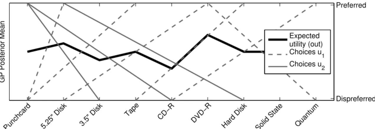
Figure 1: GPPREF result for a single user; the thick black line depicts the posterior mean

E[fu|Du,X] of the GP; dashed lines represent pairwise choices (training examples, right axis).

For example, the leftmost dashed line states that the user preferred a 5.25” floppy disk (upper end of the line) to a punchcard (lower end); the dashed lines’ thickness indicates the certainty with which the trained model reproduces the training examples. All training examples are reconstructed correctly, but the regression indicates lower certainty for the unusual training example on the far right.

of [Chu and Ghahramani, 2005b] are the definition of a plausible likelihood function for pair-wise choice data, and the description of a tractable procedure for approximating the posterior

P(fu|Du,X) as a multivariate Gaussian. One strength of the Bayesian framework is the clean separation between evidence and beliefs and, as such, other types of choice data (e.g., n-ary discrete choices) can in principle also be accommodated. We refer the interested reader to their work for technical details; in the following, we abbreviate this standard form of Gaussian process preference regression as GPPREF.

Figure 1 gives an example of applying GPPREF to pairwise choices among storage tech-nologies from a single user. The thick black line depicts the mean of the GP posterior, µu = E[fu|Du,X]. Note, that all training examples are correctly reproduced by this line. For example, the leftmost training example (5.25”_u Punchcard) is correctly reproduced because the poste-rior mean at5.25”is greater than atPunchcard. A key advantage ofGPPREFfor our purposes is its principled approach to estimating predictive uncertainties. In the figure, the thickness of the choice lines captures the certainty with which they are reproduced by the trained model. Interestingly, most choices are reproduced with high certainty except for the unusual example on the far right, which conflicts with the user’s general preference for more advanced storage technology. In an autonomous decision-making context, an agent could use this information to prompt the user to either revise or confirm the conflicting choiceDVD-R_u Quantum. Despite its advantages,GPPREFis limited when it comes to typical information systems scenarios with multiple users, because it estimates only a single posterior distribution over utility functions. To resolve this, one of two na¨ıve approaches can be followed:

1. Infer one utility function for all users simultaneously. This approach works well as long as all users share similar preferences. It fails, however, in the more probable case of heterogeneity among users. Figure 2 illustrates this situation for the two user case. 2. Infer one utility function for each user. This approach alleviates the problem of

conflicting preferences, but it only works if enough choices have been observed for each user. In other words, estimating one utility function per user misses out on an important opportunity to borrow statistical strength from like-minded users.

(11)

Punchcard 5.25" Disk 3.5" Disk

Tape _CD−R

DVD−R

Hard Disk _{Solid State} Quantum

GP Posterior Mean Dispreferred Preferred Expected utility (out) Choices u₁ Choices u₂

Figure 2: GPPREFresult for two users with conflicting preferences; even though many training examples are reconstructed correctly, the regression indicates low certainty across all training examples, and pronounced difficulties in finding a utility function that generalizes across both users.

of certainty and accuracy with minimal intrusiveness. [Jiang and Tuzhilin, 2006] have shown that, for a broad range of models, the best results in this regard are to be expected between

individual-level and population models, at the level of user segments. While it is possible to segment the user population based on, e.g., demographics and then use GPPREF on the resulting segments, this solution is unsatisfactory for both theoretical and practical reasons. On a theoretical level, demographics are likely too coarse to be a good approximation of users’ like-mindedness. It is therefore unclear whether segments derived in this way will lead to the intended gain in statistical strength. From a practical perspective, demographics may simply not be available, e.g., in online settings. A better solution would be to inducesegments based on users’ choices, but it is unclear how such an induction could proceed using pairwise choices or similarly unwieldy types of data.

3.3 Modeling Multi-User Preferences

Our mixed-effect preference model MEP facilitates probabilistic preference estimation at the segment level and it segments users based on their choices in the process. The general idea behind MEP is that the latent utility function fu for each user u is partly explained by the

effects of the user’s association with one of ns segments (segment-level effects) and partly by

idiosyncratic effects of the user himself (individual-level effects). More formally

fu(x) =szu(x) +iu(x), for u∈U (1)

where zu ∈ {1, . . . , ns} denotes the membership of user u in one of the ns segments, and the

{szu} and {iu} are Gaussian processes which capture the segment-level and individual-level

effects, respectively.

While this formulation may look superficially similar to discrete choice models, it is important to note that the {fu}, {szu}, and {iu} in our notation are stochastic processes. Most discrete

choice models assume that users’ latent utility functions come from a predetermined parametric class of functions (e.g., the class of linear functions), and they estimate the concrete parameters of the hypothesized utility function based on observed choices. In contrast, our model computes a full distribution over a broad range of utility functions without presupposing a certain function class. This formulation allows us to sidestep the question of the “true” utility function’s shape, and it yields predictive uncertainty estimates that are crucial in an autonomous decision-making context.

(12)

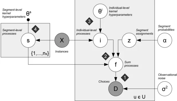
Figure 3 shows the probabilistic graphical model for MEP. Given instances X and choices

Du, our goal is to estimate a probabilistic model that describes how theDu are generated for

each user u∈U. Working backwards from theDu, this generative process proceeds as follows:

Figure 3: Probabilistic graphical model forMEP; circles indicate random variables; dark coloring indicates observed data; arrows denote probabilistic dependence; shaded platesare instantiated for each segment or user, respectively

Observed choices in Du are generated by utility functions fu ∼ GP. In an ideal world, a

user’s choices could simply be read off any concrete utility function drawn from P(fu|·). But in reality, choices will be distorted by behavioral influences and by several types of measurement errors (e.g., when users accidentally make unintended choices). These deviations are captured in the noise parameter σ2_.

Utility functionsfu are generated by summing an individual-level effectiu and a

segment-level effect szu. We model the membership of a user u in segment k as a multinomial

distribution with ns segments and segment probabilities α, that is, zu ∼ M ulti(α). The

number of segments is a user-defined input to our model. Alternatively, it could be modeled probabilistically as a Dirichlet process [Ghahramani, 2012] at the expense of additional computational cost. But, as we will show in our experiments, MEP is reasonably robust to mis-specification ofns and we therefore prefer this simpler formulation.

Individual-level effects iu ∼ GP(µu,Kiu) are generated by GPs with kernel functions Ki_u(θi

u) that describe the processes’ covariance structure. Previous researchers have

suc-cessfully used Gaussian kernels for preference estimation, e.g., [Birlutiu et al., 2012], and we follow this choice in our experiments below, while noting that our model can accom-modate any other kind of kernel as well. The kernel functions at the individual level are parametrized with parametersθi

u that are estimated from the data.

Segment-level effects sk∼ GP(µk,Ks) are generated by GPs with a common kernel

func-tion Ks(θs_{), the parameters of which are a user-defined input to the model. Generally}

speaking, the segment-level parameters will be chosen such that thesk are more adaptive

since they are estimated based on all of a segment’s users, whereas the θi

(13)

to emphasize each user’s idiosyncrasies. The fixed choice of θs _{allows us to simplify the}

inference task; below, we will only consider the maximum a-posteriori (MAP) estimates for thesk while maintaining full distributions over the iu. The Gaussian process formulation

can in this case can be thought of as a regularization on the realizations of the sk [Lu

et al., 2008, Wang et al., 2010].

In sum, we are given instances X={Xu}, choicesD ={Du}, the number of segments ns, and

the segment-level kernel functionKs with its parameters θs_{. What we are interested in finding}

is the maximum likelihood estimate Θ∗ for Θ = {α,s, σ2_{, θ}i

u} where s = {sk(X)} denotes a

random vector containing the evaluation of the segment-level GPs sk at all instances x ∈ X.

More formally we aim to find

Θ∗ = arg max

Θ P(D|X,Θ)P(s|θ

s₎ ₍₂₎

Once we have estimated Θ∗, we can answer a number of interesting queries, such as

• What is the probability that user u prefers instancex+ _{to instance}_x−_{? Here,} _x+ _and _x−

may or may not have been referenced in earlier choices by the user. In fact, x+ _and _x−

may be entirely new in the sense thatno userhas made any earlier statement about them. • What is the probability that user u belongs to segment k; or what is the most likely association between users and segments? Which users are borderline cases between two or more segments?

• What are the commonalities of all users that are likely associated with segment k?

Input: InstancesX={Xu}, choicesD={Du}, number of segments ns, segment-level

kernel parametersθs

Output: Segment-level effectss, individual-level kernel parametersθi

u, segment

assignmentszu, segment probabilitiesα, observational noise parameter σ2 Qt₌_Qt−1 ₌_−∞_;

Initialize Θ; Θt−1 _{= Θ ;} _{/* Section A.1 */}

repeat

Q(Θ,Θt−1) =E{i,z|X,D,Θt−1_}log [P(D,i,z|X,Θ)×P({s_k}|θs)] ; /* E-Step, Section

A.2 */

Θ∗= arg maxxQ(x,Θt−1) ; /* M-Step, Section A.3 */

Qt−1 ₌_Qt_;_Qt₌_Q_(Θ∗_,_Θt−1_);

Θt−1 = Θ; Θ = Θ∗;

untilQt_≈_Qt−1_;

Algorithm 1:Mixed-Effect Preference Model

The direct optimization of the objective function in Equation (2) is intractable and we therefore resort to the Expectation Maximization (EM) algorithm [Dempster et al., 1977]. The hidden variables in our model are z={zu} and i ={iu(Xu)} where iu(Xu) denotes a random

vector containing the evaluation of the GP iu at all instance x ∈ Xu that user u has stated

something about. The EM algorithm estimates the desired values in an iterative fashion where each step is guaranteed to improve the objective function, and the algorithm is guaranteed to converge to a local optimum. Algorithm 1 shows an outline of this process; full technical details are provided in Appendix A.

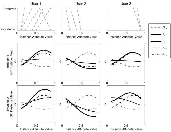
We limit the discussion of inference inMEP here to an example. Figure 4 shows two MEP

iterations for three users (columns) and two segments. The choices of each user (training exam-ples) are depicted in the top row. For example, the first user prefers an instance with attribute

(14)

0 0.5 1 Dispreferred

Preferred

Instance Attribute Value User 1

0 0.5 1

Instance Attribute Value User 2

0 0.5 1

Instance Attribute Value User 3 0 0.5 1 0 Iteration 1 GP Posterior Mean 0 0.5 1 0 0 0.5 1 0 0 0.5 1 0 Iteration 2 GP Posterior Mean

Instance Attribute Value

0 0.5 1

0

0 0.5 1

0

Du

fu

iu szu

sz¯u

Figure 4: MEP sample run for three users and two segments; each column represents one user; top row shows users’ pairwise choices, remaining rows show the first two iterations of the algorithm. Dash-dotted lines represent posterior means of the segment-level effects E[sk|D,X]

for two segments, where the highest-probability segment for each user is drawn in black. Thin black lines represent the posterior means of the individual-level effects E[iu|Du,X]; thick black lines represent the sum of the individual-level and the most likely segment-level means, see Equation (1).

(15)

value 0.2 over an instance with attribute value 0.1, which gives rise to the leftmost dashed line in the top-left panel in Figure 4. The middle and bottom rows of the figure visualize the first two iterations on these input data. There, the dash-dotted lines depict the two segment-level effects sk. We replicated these effects across all plots in each row and colored the most likely

segment assignment for the respective user black. The thin black lines represent the individual-level effects iu for each user, and the thick black lines additionally include the most probable

segment-level effect fu =iu+szu. 1

Consider the first iteration in the middle row of Figure 4. The overall utility f1 for u1

is comparable to the result of the user regression from Figure 1, but unlike the single-user case much of its general shape has now been absorbed by the segment-level effect. The individual-level effect i1 only serves to slightly increase the steepness at low attribute values.

Similarly, for u2 much of the downward-sloping tendency suggested by her choices is absorbed by the second segment-level effect. For u3 finally, only very limited observations are available.

In deciding which segment to assign the user to,MEPopts for the same segment asu1 based on

the observation that both users share the same preferences with respect to high attribute values. The individual-level effecti3 amplifies the (more conclusive) evidence foru3 in that region and

adds further to the downward sloping trend towards the right of the plot.

Such generalizations from the individual to the segment level are the driver behind MEP’s ability to make inferences from limited observations per user: by inferring that u3’s preferences so far have been similar tou1, it can make more informed statements about u3’s preferences in

the low attribute value region that the users has not stated anything about. Importantly, the

MEP estimate acknowledges the speculative nature of this generalization: while the segment assignment probabilities (not shown in the figure) are close to certainty for u1 (89%) and u2

(84%),MEPonly deems itmore likelyforu3to belong to the same segment asu1 (62%) than to

the other segment (38%, plausible based on u2’s general preference for lower attribute values). In an autonomous decision-making context, such certainty information is crucial for deciding whether a user should be prompted for additional information or not.

The second iteration in the bottom row of Figure 4 only serves to refine this estimate. During this iteration, the algorithm finds a slightly better allocation of the effects between the individual and the segment level. Specifically, the hump shape in s1 remains while more of the general

upward trend for u1 and downward trend foru3 are now captured in the individual-level effects. Similarly, more ofu2’s behavior is now captured by her individual-level effecti2as she is the only high-impact member of that segment. This behavior is typical of MEP, and we found during our experiments that it usually took three or less EM iterations to arrive at such high-quality estimates.

4 Experimental Evaluation

Given the fragile, constructed nature of human preferences, one can question the evaluation of preference models on converted ranking, rating, or regression datasets as is frequently the case in preference learning studies. For example, ranking tasks evoke a quantitative mode of reasoning in human decision-makers [Slovic, 1995] which is markedly different from the qualitative reasoning mode evoked in pairwise choices.

For this study, we collected a dedicated set of pairwise choice data in accordance with the focus of our model. Our data was collected on Amazon Mechanical Turk (MTurk,http://www. mturk.com), a crowdsourcing platform that has recently attracted attention among behavioral scientists [Buhrmester et al., 2011, Mason and Suri, 2012] but that has so far not been used

1

To keep the text uncluttered, we omit the expectation operators and the conditioning of the processes in this

example. That is, we refer to the posterior mean E[sk|D,X] of the segment-level processes as sk, and to the

posterior meanE[iu|Du,X] of the individual-level processes asiu. The reader should bear in mind, however, that

(16)

for the collection of preference data. Several scholars have studied the demographics of MTurk workers [Ipeirotis, 2010] and have proposed guidelines for assuring the quality of data collected through MTurk tasks [Paolacci et al., 2010]. These studies give reason to believe that (1) MTurk data can be of equal or better quality than data selected though channels such as student surveys, (2) MTurk workers are highly diverse (increasing external validity), and (3) the unsupervised nature of MTurk tasks may reduce the risk of experimenter bias (increasing internal validity), all if proper precautions are taken against distractions and random responses.

Our 80 adult American participants were asked to state their preferences in ten pairwise choices between electricity tariffs from the Texan retail electricity market. As a commodity, electricity is exhaustively described using a few quantifiable attributes (price per kilowatt-hour, renewable content, etc.) and unaffected by appearance or workmanship, which makes it a good object for online preference experiments. Each tariff pair was selected at random from a total of 30 tariffs. We also asked participants to answer ten questions on their demographics and electricity consumption behavior, some of which were attention checkers for which the correct answer had to be consistent with an answer given on another question. We restricted the final dataset to 58 participants who had taken three minutes or more to answer all our questions, and had passed all attention checks. Further details on the data collection process are given in Appendix B. Our interest in the experimental evaluation was threefold:

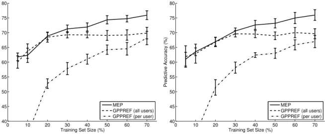
1. Predictive accuracy is a key quality indicator for preference models. We measured how well trained MEP instances performed on held-out test data compared to GPPREF

(population level and individual level) for different training set sizes.

2. The second important indicator for the autonomous decision-making task we consider is

predictive certainty. Note, that predictive certainty is also the key differentiator of our probabilistic approach. Certainty indications should be highly informative in the sense that the model should indicate high certainty on predictions that turn out to be correct and low certainty otherwise.

3. And finally, we were interested inMEP’s sensitivity to the user-defined number of segments

ns, and the segment-level kernel hyperparameterθs_.

0 10 20 30 40 50 60 70 40 45 50 55 60 65 70 75 80

Training Set Size (%)

Predictive Accuracy (%)

MEP

GPPREF (all users) GPPREF (per user)

0 10 20 30 40 50 60 70 40 45 50 55 60 65 70 75 80

Predictive Accuracy (%)

MEP

Figure 5: Predictive accuracy for MEP versus GPPREF; two segments (left) versus five seg-ments (right); error bars show confidence at the 95% level based on 10-fold cross validation;

MEP performs similar to GPPREF(all users) for limited observations and significantly better from about 3-4 pairwise choices per user; GPPREF(per user) requires significant input before predicting well and performs worse than random for limited observations

(17)

Figure 5 shows predictive accuracies on test data for MEP and GPPREF when MEP is initialized to learn two segments (left) or five segments (right). The horizontal axis shows the percentage of pairwise choices used to train the model; all remaining choices are held out for testing. The 40% point, for examples, shows runs where four out of ten choices per user (on average) are used to train the model. It is unsurprising that predictive accuracy increases as more training data become available. But MEP combines reasonable accuracy for cases with very limited data (where at best a general tendency can be estimated) with substantial accuracy growth as more choices are observed. A singleGPPREFmodel over all users, on the other hand, levels out for denser datasets because the increasing detail of these heterogeneous data cannot be captured in a single utility function. And estimating separateGPPREFmodels per user delivers unsatisfactory performance for all but the densest training sets, as these localized models do not generalize across users. In fact, the per-user estimates perform worse than random guessing for less than three observations due to strong overfitting. It is interesting to note that all aforementioned results are identical for the two and the five segment case, except for small differences in confidence interval widths.2

0 10 20 30 40 50 60 70 0 0.05 0.1 0.15 0.2 0.25 0.3 0.35 0.4

Certainty Score

MEP

0 10 20 30 40 50 60 70 0 0.05 0.1 0.15 0.2 0.25 0.3 0.35 0.4

Certainty Score

MEP

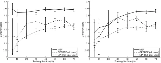
Figure 6: Certainty scores for MEP versusGPPREF; two segments (left) versus five segments (right); error bars show confidence at the 95% level based on 10-fold cross validation; certainties are strongly affected when misestimating segment numbers for limited observations, but stabilize at about 3-4 pairwise preferences per user

Figure 6 shows similar graphs for thecertainty scoresof the different models, where higher scores are better.3 MEP’s certainty estimates are highly informative in the sense that it only indicates certainty on predictions that later turn out to be correct. Interestingly, certainty scores for very limited data are more strongly affected by the of choice segments ns than predictive

accuracies. This effect is, however, simply caused by distributing very limited evidence across many segments. Beginning at about four to five training samples per user, this choice becomes inconsequential and MEP’s certainty estimates are again significantly more informative than those given by other models.

2_{We also examined}_MEP_{’s robustness with respect to different segment-level kernel parameters} _θs_{and found}

the same degree of robustness. We omit details in the interest of brevity.

3

Our certainty score is designed to capture how informative the predictive certainty output of a model is. For each test sample, we determine how far the model’s certainty indication lies from the indifference point (50%). For predictions that later turn out to be correct, the certainty indicated by the model should have been high (ideally 100%), whereas for predictions that turn out to be incorrect the opposite should be the case (ideally 0%). The certainty score is the average of these contributions over all test samples, and it therefore ranges from -0.5 (worst) to +0.5 (best).

(18)

5 Conclusions and Future Work

Models of human preferences will play an important role in the personalized, autonomous in-formation systems of the future. Useful preference models have to learn from multiple types of observations; make inferences based on limited, unobtrusively collected data; and yield confi-dence estimates so that autonomous agents can return control to their users when unsure about high-value decisions. We are gradually beginning to understand how preferences are formed based on insights from Psychology and Marketing. But the best design for a computational model that captures such inherently fragile preferences while satisfying the aforementioned re-quirements remains to be found.

Our preference model MEP is the first to combine probabilistic estimates, systematic data pooling across multiple users, flexibility with respect to different types of preference data, and a principled approach to segmentation in one coherent method. We demonstrated MEP’s ability to deliver more accurate predictions and more informative certainty indications than previous probabilistic models for pairwise choices. Importantly, we obtained our results on real-world preference data instead of converted rating datasets with artificially high internal consistency. This mirrors our intention to embrace inconsistencies, and to let them unfold in the form of uncertainties that can guide autonomous agents. We acquired this data through Amazon Me-chanical Turk, a commercial crowdsourcing platform, a practice which we have not previously encountered in preference learning. Our work confirms the finding of [Jiang and Tuzhilin, 2006] that the best predictive performances can be expected at the segment-level for the case of prob-abilistic preference models.

The work presented in this article lays the foundation for a number of interesting applications and extensions:

1. The clean separation between the internal GP representation and the observations inher-ited from GPPREF allows us to learn from other types of information besides pairwise choices. For example, choices between more than two alternatives, and contextual and temporal information could all be used to accelerate learning and improve predictive cer-tainty.

2. The principled uncertainty estimates produced by MEP can be used for active learning schemes that determine the highest-value question to ask when eliciting preferences inter-actively, thereby reducing the user’s burden, e.g., [Birlutiu et al., 2012, Saar-Tsechansky et al., 2009, Houlsby et al., 2012]. Uncertainty estimates can also serve to locate inconsis-tencies in user preferences over time. Such inconsisinconsis-tencies can point to regime shifts [Ketter et al., 2012] caused by changing tastes or more mundane causes like multiple users working from one account [Murthi and Sarkar, 2003]. We speculate that our data-driven approach to segmentation can help to identify and resolve such situations.

3. One disadvantage inherent in na¨ıve Gaussian process inference is its cubic complexity in the number of instances (on which the user made choices,|Xu|). To makeMEPpractically

applicable we are evaluating approximation schemes that overcome this deficit. Several approaches have been proposed, e.g., [Snelson and Ghahramani, 2006, Quinonero-Candela et al., 2007, Qi et al., 2010], and we are evaluating the speed versus quality tradeoffs they entail for our application.

Moreover, behavioral quality indicators, such as users’ trust in the model’s predictions, should be investigated as starting point for further improvements in user preference models, e.g., [H¨aubl and Trifts, 2000, H¨aubl and Murray, 2003, Lee and Benbasat, 2011].

Our work contributes to the foundations for next-generation information systems, and it constitutes an important step towards systems that act autonomously on their users’ behalf.

(19)

Acknowledgements The authors would like to thank Perry Groot and Tom Heskes for in-sightful discussions on probabilistic preference modeling, and for sharing their implementation of Gaussian process regression with preference likelihoods. We are also grateful for constructive comments on an earlier version of this work from four anonymous WITS 2012 reviewers. Their comments inspired, among other things, the rigorous mathematical derivation that we give for our algorithm in this paper.

APPENDIX

A

Probabilistic Inference in

MEP

We now derive the technical details required for probabilistic inference in MEP. Recall from Algorithm 1 in Section 3.3 that we are given as inputs

• instancesX={Xu},

• choicesD={Du},

• the number of segmentsns, and

• the segment-level kernel functionKs with its parameters θs_.

What we seek to infer is the maximum likelihood estimate Θ∗ for Θ ={α,s, σ2_{, θ}i

u} which we

restate here for convenience

Θ∗ = arg max

Θ P(D|X,Θ)P(s|θ

s₎ ₍₃₎

There is no analytical solution for this optimization problem and we instead resort to the Ex-pectation Maximization (EM) algorithm [Dempster et al., 1977] with hidden variablesz={zu} and i = {iu(Xu)}. Our presentation proceeds in three steps: A.1 discusses the initialization

of Θ, A.2 derives the complete-data log-likelihood Q(Θ,Θt−1) as required in the expectation step of Algorithm 1, and A.3 explains how to optimize Q(Θ,Θt−1) with respect to Θ in the maximization step.

A.1 Initialization

We follow one of the following two approaches in initializing Θ:

1. When no additional data on individual users is available, we first drawnsfunction

realiza-tions for sk from a GP prior with given parameter θs. We then determine, for each user,

the likelihood that his training observations were generated by each of thesk and initialize

α as the weighted segment probabilities over all users.

2. In the case where additional demographics on users are available, it can be leveraged for model initialization as follows: We perform a regular user segmentation by clustering users along their demographic data with an arbitrary clustering method for metric data. We then run a standard GPPREF regression (including hyperparameter estimation) on the resulting segments and initialize s using the estimated posterior means for each segment, andσ2_,_θi

u from the hyperparameter estimates. The segment probabilitiesαare initialized

(20)

A.2 Expectation Step

In the expectation step, we compute the expectation of the complete-data log-likelihood with respect to the hidden variables z and i, or formally

Q(Θ,Θt−1) =E{i,z|X,D,Θt−1_}log [P(D,i,z|X,Θ)×P({s_k}|θs)]

Our derivation is similar to that in [Wang et al., 2010] with the exception that they consider the simpler case of real-valued observations distorted by Gaussian noise, whereas in MEPwe adopt the more unwieldy noise formulation for pairwise choices from [Chu and Ghahramani, 2005b]. First, note that

P(i,z|X,D,Θt−1) =Y

u

P(iu, zu|X,D,Θt−1)

and we have that

P(iu, zu|X,D,Θt−1) =P(iu|zu,Xu,Du,Θt−1)×P(zu|Xu,Du,Θt−1) (4)

Let us consider each of the terms on the right-hand side of Equation (4) separately. The first term amounts to evaluating the posterior of a Gaussian process preference regression with a known segment-level effect szu. In other words, we perform a standard GPPREF regression

where the likelihood terms now include the segment-level effectszu

P(Du|zu,Xu,Θt−1) = nDu Y j=1 P(x+_u,j u x_u,j− |(iu+szu)(x + u,j),(iu+szu)(x − u,j)) (5)

Importantly, under the Bayesian framework, other types of data and likelihoods can also be accommodated instead of pairwise choices, as long as a tractable procedure for approximating the GP posterior exists. For the second term on the right-hand side of Equation (4) we have by Bayes’ rule that

P(zu|Xu,Du,Θt−1)∝P(zu|Θt−1)×P(Du|zu,Xu,Θt−1)

whereP(zu|Θt−1) =M ulti(αt−1_{) is known, and}_P₍_D

u|zu,Xu,Θt−1) is the likelihood of

observ-ing the choicesDuunder the segment-level effectszu. These latter likelihoods are already known

from the GPPREFregression (Equation (5)) above. Combining these results, we have that

Q=E{z,i|X,D,Θt−1_}[logP(D,i,z|X,Θ)] + logP({s_k}|θs) =E " logY u Y k P(Du|iu, zu =k,X,Θ)P(iu|zu =k,Θ)P(zu =k|Θ) # (6) + logP({sk}|θs)

Denote the expectation term in Equation (6) as ˜Q= ˜Q(Θ,Θt−1). ˜ Q(Θ,Θt−1) =E{z,i|X,D,Θt−1_}[logP(D,i,z|X,Θ)] =E{z|X,D,Θt−1_}E_{_i_|_z_,_X_,_D_,Θt−1_}[logP(D,i,z|X,Θ)] =X z P(z|X,D,Θt−1)X u X k 1[zu=k]× Z dP(iu|zu =k) log [P(Du|iu, zu=k,X,Θ)P(iu|zu=k,Θ)P(zu=k|Θ)] =X u X k X z P(z|X,D,Θt−1)1[zu =k] ! | {z } γu,k × Z . . .

(21)

Note that P

zP(z|D,X,Θt−1)1[zu =k]

=E[zu =k|Du,Xu,Θt−1] can be interpreted as the

fractional membership of user u in segment k and we will denote this term as γu,k henceforth. Substituting these results back intoQ we obtain

Q(Θ,Θt−1) = logP({sk}|θs) + ˜Q(Θ,Θt−1) = logP({sk}|θs) + X u X k γu,k× (7) h E{iu|zu=k,X,D,Θt−1}[logP(iu|zu=k,Θ)] + E{iu|zu=k,X,D,Θt−1}[logP(Du|iu, zu=k,X,Θ)] + E{iu|zu=k,X,D,Θt−1}[logP(zu=k|Θ)] i

A.3 Maximization Step

In the maximization step we aim to optimize Θ∗ = arg max

Θ Q(Θ,Θ t−1₎

This problem can be decomposed into three separate optimization problems by separating the terms from Equation (7) into Q=Q1+Q2+Q3 as follows:

Q1(Θ,Θt−1) = X u X k γu,k ×E{iu|zu=k,X,D,Θt−1}[logP(zu =k|Θ)] (8) Q2(Θ,Θt−1) = logP({sk}|θs)+ (9) X u X k

γu,k×E{iu|zu=k,X,D,Θt−1}[logP(Du|iu, zu =k,X,Θ)]

Q3(Θ,Θt−1) =X

u

X

k

γu,k ×E{iu|zu=k,X,D,Θt−1}[logP(iu|zu=k,Θ)] (10)

We now address the optimization of each of these terms in turn.

A.3.1 Optimizing α (Q1)

Note that P(zu = k|Θ) =αk and, hence, optimizingQ1 amounts to the following constrained

optimization problem: max α X u X k γu,k×logαk s.t.X k αk= 1

Computing the derivatives of the Lagrangian, we obtain the following system of equations

∂ ∂αi " X u X k [γu,k×logαk] +λ X k αk−1 !# = " X u γu,i αi +λ # i ! = 0

The solution to which is αi=−_λ1Puγu,i. We know that

1=! X k αk=−X k 1 λ X u γu,k ! =−1 λ X k X u γu,k =−1 λ X u 1

which means that λ=−nu and

αi= 1

nu

X

u γu,i

(22)

A.3.2 Optimizing s, σ2 ₍_Q 2)

In the next step, we considersto be the (ns×nx)-elements column vector of segment-level effect

values where each segment-level effectsk is evaluated at allx∈X. We denote asskall elements

of sthat pertain to thek-th segment, and assk,i the single element that pertains to instancexi

and segmentk. Expanding the expectation term in Q2 yields E{iu|zu=k,X,D,Θt−1}[logP(Du|iu, zu =k,X,Θ)] = Z iu P(iu|·)× nDu X j=1 logP(x+ u,j u x−u,j|sk, σ2)diu = Z iu P(iu|·)× nDu X j=1 log Φ i++s+−i−−s− √ 2σ sk, σ 2 diu (11)

where Φ stands for the CDF of a standard Gaussian and the last step in Equation (11) uses the definition of the pairwise choice likelihood from [Chu and Ghahramani, 2005b]. The integral above has no closed-form solution but it can be approximated using Gauss-Hermite quadrature where we take P(iu|·) to be the envelope function. Note, that Gauss-Hermite quadrature in general would require the computation of nx nested sums, where nx is the number of instances or, alternatively, the number of elements in iu. However, by realizing that (a) each element of Du makes use of only two components ofiu (namely its evaluationi+ at the preferred andi−at

the dispreferred instance), and that (b) the marginal ofiu with respect to these two dimensions is a bivariate Gaussian we can rewrite the integral as

nDu X j=1 Z d(i+,i−) P(i+, i−|·)×log Φ i++s+−i−−s− √ 2σ sk, σ 2 d(i+, i−) (12)

where the integral is now an integral over the density of a bivariate Gaussian. One last correction relates to the correlation structure of the (i+, i−). In general, the (i+, i−) are jointly Gaussian

with mean (µ+, µ−) a correlation that is reflected in the posterior covariance matrix of their

Gaussian process iu. Using the transform • t+= i+_σ+−µ+ ⇒i+(t+) =t+σ++µ+ • t−= i−−µ−−ρi+ σ− √ 1−ρ2 ⇒i−(t+, t−) =t−σ− p 1−ρ2₊_ρ₍_t+σ+₊_µ+_{) +}_µ₋ where σ2

+, σ−2, and ρ are the variances of i+ and i− and their correlation, respectively, we

obtain two uncorrelated and independent Gaussians. Following [Varin et al., 2005] we rewrite integral (12) as 1 2π nDu X j=1 Z t− Z t+ log Φ i+(t+) +s+−i−(t−)−s− √ 2σ sk, σ 2 e −t2₊ 2 e −t2₋ 2 dt₊dt₋ ≈ 1 2π nDu X j=1 M X m1=1 M X m2=1 log Φi+(hm1) +s+√−i−(hm2)−s− 2σ sk, σ 2 | {z } =:vj × 1[wm1wm2 > ]×wm1wm2 | {z } :=Wm₁,m₂

where the h are the quadrature nodes, w the corresponding quadrature weights, and M the number of quadrature terms used. As many of the products wm1wm2 will be close to zero, it

(23)

is common to use some form of pruning [Jaeckel, 2005] to further reduce the computational requirements of the approximation. Above we used the indicator function to include only prod-ucts greater than a fixed given value . Towards the optimization ofQ2, we can now compute

its derivatives with respect to s and σ. We first consider the derivative w.r.t. sk,i, the i-th

component of the k-th segment-level effect:4

∂Q2(Θ,Θt−1) ∂sk,i ≈ ∂logP(s|θ s₎ ∂sk,i + (13) 1 2π ∂ ∂sk,i   X u X k γu,k× nDu X j=1 M X m1,m2=1 log Φ(vj)×Wm1,m2  

Here, the first term is simply the i-th component of the derivative of a multivariate Gaussian log density: ∂logP(s|θs₎ ∂sk = P(sk|θ s₎ P(sk|θs) × −Σ−_s1(sk−~0) =−Σ−s1sk

From the second term in Equation (13), summations over segments other than k disappear, as do choices in Du that do not involve instancei. Overall, we obtain

1 2π ∂ ∂sk,i X u γu,k× X j∈Du i M X m1,m2=1 log Φ(vj)×Wm1,m2 = 1 2π X u γu,k× X j∈Du i M X m1,m2=1 pj_√(sk,i) 2σ N(vj) Φ(vj) ×Wm1,m2

where N represents the standard Gaussian density, and

pj(sk,i) =     

1 ifxi is the preferred instance in statementj

−1 ifxi is the dispreferred instance in statementj

0 otherwise

While optimizing Q2 w.r.t. σ we need to ensure that σ remains strictly positive. Instead of explicitly incorporating this constraint into the optimization, we optimize w.r.t. log(σ). The corresponding first derivative is

∂Q2(Θ,Θt−1) ∂log(σ) ≈ 1 2π ∂ ∂log(σ) X u X k γu,k × nDu X j=1 M X m1,m2=1 log Φ(vj)×Wm1,m2 = 1 2π X u . . . M X m1,m2=1 N(vj)×(−vj) Φ(vj) ×Wm1,m2 To summarize: Q2(Θ,Θt−1)≈X k logP(sk|θs) + X u X k γu,k 2π × nDu X j=1 M X m1,m2=1 log Φ(vj)×Wm1,m2 (14) ∂Q2(Θ,Θt−1) ∂sk,i ≈(−Σ−_s1×sk)i+ 1 2π X u γu,k× X j∈Du i M X m1,m2=1 pj_√(sk,i) 2σ N(vj) Φ(vj) ×Wm1,m2 (15) ∂Q2(Θ,Θt−1) ∂log(σ) ≈ 1 2π X u X k γu,k× nDu X j=1 M X m1,m2=1 N(vj)×(−vj) Φ(vj) ×Wm1,m2 (16)

4_{Recall that the}_s

(24)

A.3.3 Optimizing θi ₍_Q 3)

Lastly, we wish to find

θi∗ = arg max θi Q3(Θ,Θ t−1₎ = arg max θi X u X k γu,k×E{iu|zu=k,X,D,Θt−1}[logP(iu|zu =k,Θ)] (17)

whereP(iu|zu =k,Θ) is the approximate posterior of the Gaussian process preference regression from Equation (4). In other words, iu|zu = k,Θ is distributed N(µu,k,Σu) for some µu,k = E[iu|zu = k,Θ] and Σu = Σu(θi). Expanding the Gaussian density in Equation (17) and

collecting constant terms we obtain X u X k γu,kE{iu|zu=k,X,D,Θt−1}[logP(iu|zu =k,Θ)] =C−1 2 X u log|Σu| −1 2 X u X k γu,kE{iu|zu=k,X,D,Θt−1} (x−µu,k)TΣu−1(x−µu,k)

Note, that the expectation is over the posterior, conditional on the previous parameters Θt−1. Since the µu,k are constants under this expectation, we have that E[x−µu,k] = E[x] =: µt_u,k−1

and V ar(x−µu,k) = V ar(x) =: Cut−1. Recall that for the expectation of a quadratic form we

have E[vT_Av_{] =} _tr₍_AV_{) +}_mT_Am _where _E_[_v_{] =} _m _and _{V ar}₍_v_{) =} _V_{. Applying this result to} E{iu|zu=k,X,D,Θt−1}[. . .] with v = (x−µu,k) and A = Σ

−1

u we obtain E[. . .] = tr[Σu−1(Cut−1 + µt_u,k−1(µt_u,k−1)T)], and hence the optimization task amounts to finding:

θi∗ = arg max θi Q3(Θ,Θ t−1₎ = arg max θi − 1 2 X u logΣ_u(θi_u) − 1 2 X u X k γu,k×trhΣu(θui) −1_Ct−1 u +µt −1 u,k(µ t−1 u,k) Ti ₍₁₈₎

Evaluation of this function is expensive. Computing the log determinant and solving the linear system of equations in Equation (18) require a Cholesky decomposition of each Σu which scales

as O(n3

x) with the number of instances. In our experiments, we assumed that all users within

a segment share the same kernel parameters θi_{, thereby reducing the}_number _{of evaluations of}

(18). Alternatively, thecostof evaluation can be reduced through approximations, e.g., [Snelson and Ghahramani, 2006].

B

Experimental Details

We collected the dataset used in Section 4 using Amazon Mechanical Turk (MTurk, http: //www.mturk.com), a commercial crowdsourcing platform. Eighty adult American participants were invited to fill in an academic survey about their electricity tariff preferences5 _{in exchange}

for a payment of $0.30. All American MTurk workers could theoretically preview our survey through the MTurk platform, and 80 workers ultimately self-selected to participate. The survey consisted of three parts:

1. First, we reviewed basic electricity tariff concepts: fixed, variable, and indexed tariffs; and tariffs guaranteeing that a certain percentage of delivered electricity is produced from renewable sources.

(25)

Table 2: Example choice situation. Each participant in our experiment made ten choices. Imagine having to choose between the following two tariffs for the household that you currently spend most of your time in. Which one would you prefer?

1. A Fixed tariff with 100 percent renewable energy content. Your monthly cost of electricity will be

• 57.00$ if you consume 500 kWh, • 106.00$ if you consume 1000 kWh, and • 204.00$ if you consume 2000 kWh

under this tariff. You pay your monthly electricity bill at the end of each month. A 12 months notice period applies before you can cancel this tariff.

2. A Variable tariff with 0 percent renewable energy content. The cost of electricity in the first month will be

• 54.50$ if you consume 500 kWh, • 101.00$ if you consume 1000 kWh, and • 194.00$ if you consume 2000 kWh

under this tariff. After the first month, the price of electricity may go up or down in accordance with the tariff’s terms (and within legal bounds). You will have to pre-pay your monthly electricity bill at the beginning of the month. You can cancel your tariff anytime.

(26)

2. Next, participants were asked to make ten choices between pairs of tariffs, see Table 2 for an example. Each pair was randomly generated from a total of thirty tariffs that we kept constant throughout. The set of thirty, in turn, was randomly selected from over 230 tariffs offered in Austin, Texas in February 2013. We chose to work with a subset of all available tariffs to keep the number of required participants manageable. Texas has one of the most advanced competitive retail electricity markets in the United States and provides daily information on available tariffs, seehttp://www.powertochoose.org.

3. Finally we asked participants to answer ten questions on their demographics and electricity consumption behavior, some of which were attention checkers for which the correct answer had to be consistent with an answer given on another question.

Participants had a maximum of thirty minutes to fill out all questions, but could submit their results before that time. Participants could also withdraw, allowing another MTurk worker to fill out the survey instead. Next to the given answers, we recorded the time between self-selecting for participation and the submission of results. In pretests among colleagues, we had established that it took a quick reader at least three minutes to process all provided information. We therefore discarded surveys submitted before that time. As a further safeguard against random answers, we asked two pairs of attention check questions in the demographics section where the answers to one question depended on the answer of the other. We also discarded surveys where at least one of the attention check pairs was answered inconsistently, leaving us with a total of 58 surveys that met our quality standards.

References

Gediminas Adomavicius and Alexander Tuzhilin. Toward the next generation of recommender systems: A survey of the state-of-the-art and possible extensions. IEEE Transactions on Knowledge and Data Engineering, pages 734–749, 2005a.

Gediminas Adomavicius and Alexander Tuzhilin. Personalization technologies: a process-oriented perspective. Communications of the ACM, 48(10):83–90, 2005b.

Gediminas Adomavicius and Alexander Tuzhilin. Context-aware recommender systems. In

Recommender Systems Handbook, pages 217–253. Springer, 2011.

Greg M. Allenby and Peter E. Rossi. Marketing models of consumer heterogeneity. Journal of Econometrics, 89(1):57–78, 1998.

Asim Ansari, Skander Essegaier, and Rajeev Kohli. Internet recommendation systems. Journal of Marketing Research, 37(3):363–375, 2000.

Pelin Atahan and Sumit Sarkar. Accelerated learning of user profiles. Management Science, 57 (2):215–239, 2011.

Martin Bichler, Alok Gupta, and Wolfgang Ketter. Designing smart markets. Information Systems Research, 21(4):688–699, 2010.

Adriana Birlutiu, Perry Groot, and Tom Heskes. Efficiently learning the preferences of people.

Machine Learning, pages 1–28, 2012.

Edwin Bonilla, Shengbo Guo, and Scott Sanner. Gaussian process preference elicitation. Neural Information Processing Systems, 2010.

Craig Boutilier, Ronen I. Brafman, Carmel Domshlak, Holger H. Hoos, and David Poole. CP-nets: A tool for representing and reasoning with conditional ceteris paribus preference state-ments. Journal of Artificial Intelligence Research, pages 135–191, 2004.

(27)

Ronald J. Brachman. Systems that know what they’re doing. IEEE Intelligent Systems, 17(6): 67–71, 2002.

Ronen Brafman and Carmel Domshlak. Preference handling - an introductory tutorial. AI Magazine, 30(1):58–86, 2009.

Michael Buhrmester, Tracy Kwang, and Samuel D. Gosling. Amazon’s mechanical turk: A new source of inexpensive, yet high-quality, data? Perspectives on Psychological Science, 6(1):3–5, 2011.

Rich Caruana. Multitask learning. Machine Learning, 28(1):41–75, 1997.

Yann Chevaleyre, Frédéric Koriche, Jérôme Lang, Jérôme Mengin, and Bruno Zanuttini. Learn-ing ordinal preferences on multiattribute domains: The case of CP-nets. InPreference Learn-ing, pages 273–296. Springer, 2011.

Wei Chu and Zoubin Ghahramani. Gaussian processes for ordinal regression. The Journal of Machine Learning Research, 6:1019–1041, 2005a.

Wei Chu and Zoubin Ghahramani. Preference learning with Gaussian processes. InProceedings of the 22nd international conference on Machine Learning, pages 137–144. ACM, 2005b. Thomas H Davenport and Jeanne G Harris. Automated decision making comes of age. MIT

Sloan Management Review, 46(4):83, 2005.

Arthur P Dempster, Nan M Laird, and Donald B Rubin. Maximum likelihood from incomplete data via the em algorithm. Journal of the Royal Statistical Society. Series B (Methodological), pages 1–38, 1977.

Theodoros Evgeniou, Massimiliano Pontil, and Olivier Toubia. A convex optimization approach to modeling consumer heterogeneity in conjoint estimation.Marketing Science, 26(6):805–818, 2007.

Johannes F¨urnkranz and Eyke H¨ullermeier. Preference learning. Springer, 2011.

Zoubin Ghahramani. Bayesian nonparametrics and the probabilistic approach to modelling. 2012.

William Greene. Econometric Analysis. Prentice Hall, 7th edition, 2012.

Gerald H¨aubl and Kyle B Murray. Preference construction and persistence in digital market-places: The role of electronic recommendation agents. Journal of Consumer Psychology, 13 (1&2):75–91, 2003.

Gerald H¨aubl and Valerie Trifts. Consumer decision making in online shopping environments: The effects of interactive decision aids. Marketing Science, 19(1):4–21, 2000.

Alan R. Hevner, Salvatore T. March, Jinsoo Park, and Sudha Ram. Design Science in Informa-tion Systems research. Management Information Systems Quarterly, 28(1):75–105, 2004. Neil Houlsby, Jose M. Hernandez-Lobato, Ferenc Huszar, and Zoubin Ghahramani.

Collabora-tive Gaussian processes for preference learning. Advances in Neural Information Processing Systems, 2012.

Zan Huang, Huimin Zhao, and Dan Zhu. Two new prediction-driven approaches to discrete choice prediction. ACM Transactions on Management Information Systems, 3(2):9:1–9:32, July 2012. ISSN 2158-656X. doi: 10.1145/2229156.2229159.