Light Beam Search Based Multi-objective Optimization using
Evolutionary Algorithms
Kalyanmoy Deb and Abhay Kumar
KanGAL Report Number 2007005
Abstract— For the past decade or so, evolutionary multi-objective optimization (EMO) methodologies have earned wide popularity for solving complex practical optimization problems, simply due to their ability to find a representative set of Pareto-optimal solutions for mostly two, three, and some extent to four and five-objective optimization problems. Recently, emphasis has been made in addressing the decision-making activities in arriving at a single preferred solution. The multiple criteria decision making (MCDM) literature offers a number of possibilities for such a task involving user preferences which can be supplied in different forms. This paper presents an interactive methodology for finding a preferred set of solutions, instead of the complete Pareto-optimal frontier, by incorporating preference information of the decision maker. Particularly, we borrow the concept of light beam search and combine it with the NSGA-II procedure. The working of this procedure has been demonstrated on a set of test problems and on engineering design problems having two to ten objectives, where the obtained solutions are found to match with the true Pareto-optimal solutions. The results highlight the utility of this approach towards eventually facilitating a better and more reliable optimization-cum-decision-making task.
I. INTRODUCTION
In the recent past, much efforts have been put in combining evolutionary multi-objective optimization (EMO) method-ologies with a multi-criterion decision-making (MCDM) strategy in finding a set of Pareto-optimal solutions and then choosing a single preferred solution [7], [6], [11], [9]. This paper is another effort in this direction, but uses the so-called light beam methodology [8] of MCDM strategies along with the popularly-used NSGA-II procedure [4].
Interactive methodologies involving the designer or a decision-maker have been actively pursued in the field of multi-objective optimization in the recent past. In the clas-sical multi-objective optimization literature, during the past four decades, more than a dozen of interactive methodologies have been proposed. In most of these methods, some initial preference information is given by the decision-maker (DM). The algorithm then finds and presents one or more Pareto-optimal solutions satisfying the preference information pro-vided by the DM. This allows the DM to analyze the solutions and offers the DM to change his/her decision, if he/she is not completely satisfied. He/she can then change the preference information or specify more information and K Deb, Kanpur Genetic Algorithms Laboratory (KanGAL), Department of Mechanical Engineering, Indian Institute of Technology, Kanpur, India (email: [email protected])
Abhay Kumar, Kanpur Genetic Algorithms Laboratory (KanGAL), De-partment of Mechanical Engineering, Indian Institute of Technology, Kan-pur, India (email: [email protected])
do further iterations till a satisfactory solution is achieved. In some of these methods, preference information is given by specifying an aspiration or a reference point. In other methods, aspiration level is expressed based upon the trade-off rate information or by comparing two or more solutions. On the other hand, EMO methodologies are found to be adequate in finding multiple and widely-distributed trade-off solutions in a single simulation. Thus, an ideal usage of EMO lies in the steps of a MCDM procedure which require multiple evaluation of different Pareto-optimal so-lutions. For example, in the reference point based EMO suggested elsewhere [7], Pareto-optimal solutions close to the optimal solution to the achievement scalarizing function computed from the supplied reference point were found using II. In the suggested reference direction based NSGA-II procedure [6], Pareto-optimal solution corresponding to the reference points on a reference direction (dictated by two supplied points in the objective space) were found simultaneously. In this paper, we follow the light beam search procedure and instead of finding a single Pareto-optimal solution corresponding to the intersection of a line joining the supplied aspiration and reservation points and the Pareto-optimal front, we find a set of solutions in the vicinity to provide a region of interest to the DM. The light beam search procedure was proposed by Jaszkiewicz and Slowinski [8]. The basic setting is identical to the reference point method of Wierzbicki [12] in the spirit of satisfying decision making. It is analogous to projecting a focussed beam of light from an aspiration point on to the Pareto-optimal front, in the direction of a reservation point.
In the remainder of this paper, we briefly discuss the clas-sical interactive multi-objective optimization methodologies and then suggest the hybrid light beam search based EMO procedure. Thereafter, we demonstrate the working principle of the hybrid procedure on a number of test problems and engineering design problems. The problems involve two to ten objectives and a number of constraints. The paper ends with a number of conclusions and extensions to this study.
II. PREFERENCEBASEDEVOLUTIONARY MULTI-OBJECTIVEOPTIMIZATION
For a decade or so, researchers in the field of evolutionary multi-objective optimization (EMO) have shown interests in developing EMO based interactive methods. Many prefer-ence based methods have also been proposed. Phelps and Koksalan [10] have proposed a method where a pair-wise comparison is used to include DM’s preference. Branke et
al. [2] and Branke and Deb [1] have proposed a guided multi-objective evolutionary algorithm (G-MOEA), where the defi-nition of dominance has been modified based upon the DM’s preference information. Deb et al. [7], [6] have proposed the reference point based and reference direction based EMO procedures. Thiele et al. [11] have proposed a preference-based interactive EMO (PBEA). In this method, initially a rough approximated Pareto-optimal front is presented to the DM. Thereafter, the DM specifies a reference point to focus the search to his/her region of interest.
One of the advantages with most of these interactive EMO methodologies is that they attempt to find a set of preferred solutions or locate a preferred region on the Pareto-optimal frontier, instead of finding a single preferred solution. With the knowledge of multiple solutions near the region of interest, the DM will be in a better position to make a satisfactory decision. Another advantage with interactive EMO procedures is that instead of finding one or more preferred solutions near a single region of the Pareto-optimal front, an EMO can help find multiple preferred regions corresponding to different preferences simultaneously. This facility becomes handy in cases where the DM is hesitant to provide a single preferred information (such as a single reference point or a single reference direction etc.), sim-ply because he/she is not confident yet in making such a bold decision. Although, multiple yet different preference information can be considered serially one at a time before making a final choice, the EMO based procedures allow one to consider multiple (two or more) different preference information simultaneously.
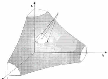
III. THELIGHTBEAMSEARCHAPPROACH The light beam search (LBS), as described in Jaszkiewicz and Slowinski [8], combines the reference point idea and tools of multi-attribute decision analysis (MADA). It enables an interactive analysis of multiple-objective decision prob-lems due to presentation of samples of a large set of non-dominated points to the decision maker in each iteration. An aspiration and a reservation point must be supplied by the DM. These two points determines the direction of the search in an iteration. If these two points are not suggested, the ideal point and the nadir point or some other worse points can be assumed as aspiration and reservation points, respectively. Initially a non-dominated middle point is determined by projecting the aspiration point on to the non-dominated front by using an augmented version of Wierzbicki’s scalarizing achievement function. Thereafter, a local preference model in the form of an outranking relation S is used to obtain neighboring solutions of the current non-dominated point, or the middle point. It is said thataoutranksb(oraSb), ifais considered to be at least as good asb. To define outranking relation, DM has to specify three preference thresholds for each objective. They are indifference threshold, preference threshold and veto threshold. In the LBS procedure, they are assumed to provide only local information, thus they are as-sumed to be constants. Based on these values, the outranking relation finds a solution which is incomparable or indifferent
to the middle point. It determines only those solutions which outrank the middle point. All such solutions constitute the outranking neighborhood of the middle point. The extreme points or characteristic neighbors are found one for each objective by considering the maximum allowed improvement in a particular objective in relation to the middle point. The DM can control the search by either modifying the aspiration and/or reservation points, or by shifting the middle point to selected better point from its neighborhood or by modifying the preference threshold values.
f3
f1
f2
Fig. 1. The light beam search approach is shown.
The following LBS procedure was suggested:
1) Ask the DM to specify starting aspiration and reserva-tion points.
2) Compute the starting middle point on the Pareto-optimal front.
3) Ask DM to specify the local preferential information used to build an outranking relation.
4) Present the middle point to the DM.
5) Calculate the characteristic neighbors of the middle point and present them to the DM.
6) If DM is satisfied, terminate the procedure, else ask DM to choose one of the neighboring points to be the new middle point, or to update the preferential information, or to define new aspiration point and/or reservation point. The algorithm proceeds by moving to to step 4.
IV. LBSBASEDEMO
With the above principle of the LBS procedure, we now propose an EMO methodology by which a set of Pareto-optimal solutions in the neighborhood of the middle point can be found using the modified outranking relation. In the original LBS method, the decision-maker has to specify three preference parameters for each objective, which is quite demanding on the part of the DM. Thus, to reduce the input parameter requirement, we use only the veto preference parameter here.
In the original LBS procedure, once the middle point is obtained, the feasible direction of the largest improvement of each objective is determined. The best feasible point in each direction, satisfying the outranking criterion is determined. These points are then projected onto the Pareto-optimal front by solving augmented form of Wierzbicki’s achievement scalarizing problem. This results in the best feasible point in each direction, satisfying the outranking criterion and Pareto-optimality.
Since the EMO approach deals with a population of solu-tions, the required points satisfying the outranking criterion in all the directions would be obtained in one simulation run. It can also find multiple preferred regions of the Pareto-optimal front corresponding to multiple light beams in one iteration, if desired by the DM. In this paper, to demonstrate the ability of the suggested procedure we shall choose any two points as aspiration and reservation points, respectively, instead of ideal and nadir point always.
To implement the procedure, we use NSGA-II as an EMO procedure, although other methods can also be tried. The following procedure is suggested for minimization problems: 1) Non-domination ranking is done for the whole
popu-lation.
2) For each front, each solution in the front is assigned a crowding rank:
a) Crowding distance (d) of each solution is calcu-lated as: d= max{λj(fj−zjr)}+ρ M X j=1 (fj−zjr), (1) wherezr = [zr
1, . . . , zMr ] is the aspiration point, Λ = [λ1, . . . , λM] is a weighting vector, λj >
0, j = 1, . . . , M and ρ is a sufficiently small positive number (called the augmentation coeffi-cient, which we have fixed to 10−6
here). The weighting vector can be defined by aspirationzr
and reservation zv points, such that zr j < z
v j, j= 1, . . . , M in the following manner:
λj = 1 zv j −z r j . (2)
b) Solution with least d value is the middle point (zc), and it is assigned the highest crowding rank. c) All the solutions which outrank the middle point are found using the outranking relation (described later).
d) For all the solutions which outrank the middle point, the maximum difference in objective value withzc is determined, as follows:
δ= max(fj−zjc), j= 1, . . . , M. (3)
Based upon the δ value, a crowding rank is assigned to each solution. A solution with lesser δ is assigned a higher rank and vice versa.
e) Remaining solutions are assigned lesser crowding rank so that they are not preferred during the selection procedure.
In case of multiple light beams, a crowding rank corresponding to each light beam is first determined for each solution. Thereafter, the minimum rank for all light beams is assigned as the final crowding rank of the particular solution.
3) To obtain a uniform distribution of solutions in the lighted region, no two solutions apart by less than distance are preferred.
The modified outranking relation used here is given below: mv(zc,f) = card{j:fj−zcj≥vj, j = 1, . . . , M},
fSzc, ifmv= 0.
The solutionf outrankszc (that is,fSzc) meansf is as good as zc. As both solutions belong to the same non-dominated
front, if f is better than zc in some objectives, then it must
be worse in at least in one other objective. Forf to outrank zc, the amount of deterioration off overzc must not exceed
the supplied veto threshold.
V. SIMULATIONRESULTS
Simulation results on two to ten objective problems are presented in this section. First, some test problems have been considered followed by a few standard engineering design optimization problems. In all simulation runs, the SBX recombination operator has been used with a distribution index of10and the polynomial mutation with a distribution index of 20 [3]. We use populations of size 100, 200, 200, and 500 for two, three, five and ten objectives, respectively. A. Two-Objective Test problem ZDT1
First, we consider the 30-variable ZDT1 problem. This problem has a convex Pareto-optimal front spanning con-tinuously in f1 ∈[0,1]and follows a function relationship:
f2= 1−√f1. Figure 2 shows various terms used for the LBS
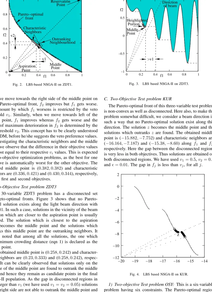
procedure. The ideal point is assumed as the aspiration point and the nadir point is assumed as the reservation point, in this case. It can be observed that the middle point is obtained by projecting the aspiration point on to the Pareto-optimal front in the direction of the reservation point. Neighboring solutions are obtained by the outranking relation. The span of the light beam on the Pareto-optimal front is determined by the veto threshold (v). We have usedv1=v2= 0.05and
= 0.01 here. It is clear that with a small v, the range of obtained solutions are also small. Thus, if the DM is interested in obtaining a large neighborhood of solutions near the desired region, a large value of the veto threshold vectorv
is required to be chosen. By using different aspiration and/or reservation points, different regions of the Pareto-optimal front can also be easily obtained. But, it may be a better strategy to assume the ideal point as the aspiration point and use different points in the objective space as the reservation point to explore different parts of the Pareto-optimal frontier.
f1 f2 front Pareto−optimal Reservation Neighbourhood Aspiration Point Point Characteristic Outranking Point Middle v1 v2 Neighbors 0 0.2 0.4 0.6 0.8 1 0 0.2 0.4 0.6 0.8 1
Fig. 2. LBS-based NSGA-II on ZDT1.
As we move towards the right side of the middle point on to the Pareto-optimal front, f2 improves butf1 gets worse.
The amount by which f1 worsens is restricted by the veto
threshold v1. Similarly, when we move towards left of the
middle point, f1 improves whereas f2 gets worse and the
extent of maximum deterioration inf2is determined by the
veto thresholdv2. This concept has to be clearly understood
by the DM, before he/she suggests the veto preference values. By investigating the characteristic neighbors and the middle point, we observe that the difference in their objective values is almost equal to their respectivevivalues. This is expected
for two-objective optimization problems, as the best for one objective is automatically worst for the other objective. The obtained middle point is (0.382,0.382) and characteristic neighbors are (0.336,0.421) and (0.430,0.344), respectively, for the first and second objectives.
B. Two-Objective Test problem ZDT3
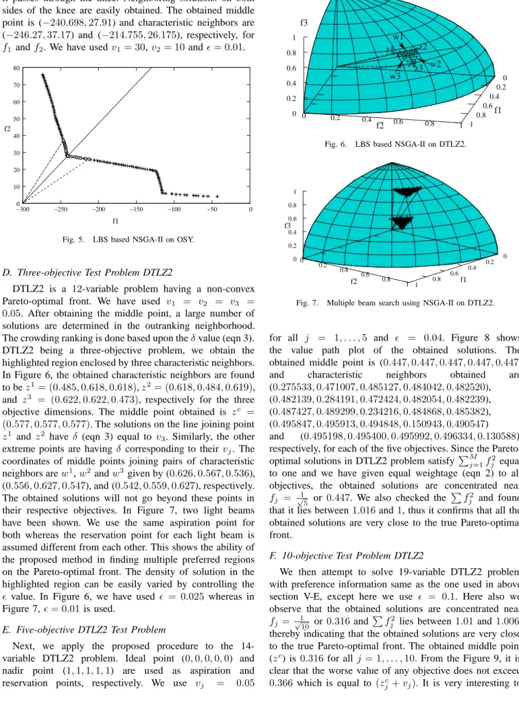
The 30-variable ZDT3 problem has a disconnected set of optimal fronts. Figure 3 shows that no Pareto-optimal solution exists along the light beam direction with = 0.01. In such a case, solutions in the vicinity of the beam direction which are closer to the aspiration point is usually obtained. The solution which is closest to the aspiration point becomes the middle point and the solutions which outranks this middle point are the outranking neighbors. It can be noted that among all the solutions, the one which has minimum crowding distance (eqn 1) is declared as the middle point.
The obtained middle point is (0.258,0.242) and character-istic neighbors are (0.23,0.333) and (0.258,0.242), respec-tively. It can be clearly observed that solutions only on the left side of the middle point are found to outrank the middle point and hence they remain as candidate points in the final NSGA-II population. As the gap in disconnected regions in f1is larger thanv1(we have usedv1=v2= 0.05) solutions
on the right side are not able to outrank the middle point and hence they cannot be present in the obtained set along with the middle point.
f1 f2 Heighlighted Portion Direction of beam Middle Point >v1 −1 −0.5 0 0.5 1 0 0.2 0.4 0.6 0.8 1
Fig. 3. LBS based NSGA-II on ZDT3.
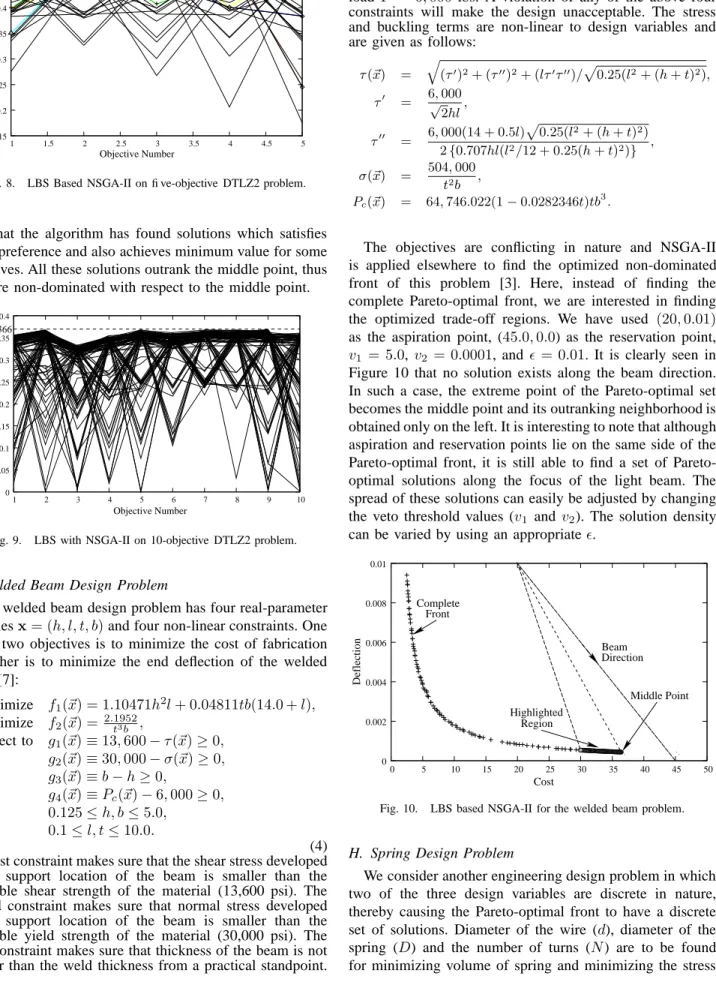
C. Two-Objective Test problem KUR
The Pareto-optimal front of this three-variable test problem is non-convex as well as disconnected. Here also, to make the problem somewhat difficult, we consider a beam direction in such a way that no Pareto-optimal solution exist along this direction. The solution z becomes the middle point and the solutions which outranksz are found. The obtained middle point is (−15.882,−7.752) and characteristic neighbors are (−16.164,−7.187) and (−15.38,−8.60) along f1 and f2,
respectively. Here the gap between the disconnected regions is very less in both objectives. Thus solutions are obtained on both disconnected regions. We have usedv1= 0.5,v2= 0.8
and= 0.01. The gap infj is less thanvj, for allj.
z
−12 −10 −8 −6 −4 −2 0 2 −20 −19 −18 −17 −16 −15 −14Fig. 4. LBS based NSGA-II on KUR.
1) Two-objective Test problem OSY: This is a six-variable problem having six constraints. The Pareto-optimal region is a concatenation of five regions. To make the task chal-lenging, we choose the beam direction in such a way that
it passes through the knee. Neighboring solutions on both sides of the knee are easily obtained. The obtained middle point is (−240.698,27.91) and characteristic neighbors are (−246.27,37.17) and (−214.755,26.175), respectively, for f1 andf2. We have usedv1= 30,v2= 10and= 0.01.
f1 f2 0 10 20 30 40 50 60 70 80 −300 −250 −200 −150 −100 −50 0
Fig. 5. LBS based NSGA-II on OSY.
D. Three-objective Test Problem DTLZ2
DTLZ2 is a 12-variable problem having a non-convex Pareto-optimal front. We have used v1 = v2 = v3 =
0.05. After obtaining the middle point, a large number of solutions are determined in the outranking neighborhood. The crowding ranking is done based upon theδvalue (eqn 3). DTLZ2 being a three-objective problem, we obtain the highlighted region enclosed by three characteristic neighbors. In Figure 6, the obtained characteristic neighbors are found to bez1
= (0.485,0.618,0.618),z2
= (0.618,0.484,0.619), and z3
= (0.622,0.622,0.473), respectively for the three objective dimensions. The middle point obtained is zc =
(0.577,0.577,0.577). The solutions on the line joining point z1
and z2
have δ (eqn 3) equal to v3. Similarly, the other
extreme points are havingδ corresponding to theirvj. The
coordinates of middle points joining pairs of characteristic neighbors arew1
,w2
andw3
given by (0.626,0.567,0.536), (0.556,0.627,0.547), and (0.542,0.559,0.627), respectively. The obtained solutions will not go beyond these points in their respective objectives. In Figure 7, two light beams have been shown. We use the same aspiration point for both whereas the reservation point for each light beam is assumed different from each other. This shows the ability of the proposed method in finding multiple preferred regions on the Pareto-optimal front. The density of solution in the highlighted region can be easily varied by controlling the value. In Figure 6, we have used = 0.025 whereas in Figure 7, = 0.01 is used.
E. Five-objective DTLZ2 Test Problem
Next, we apply the proposed procedure to the 14-variable DTLZ2 problem. Ideal point (0,0,0,0,0) and nadir point (1,1,1,1,1) are used as aspiration and reservation points, respectively. We use vj = 0.05
f1 f2 f3 z2 z1 z3 w1 w2 w3 0 0.2 0.4 0.6 0.8 1 0 0.2 0.4 0.6 0.8 1 0 0.2 0.4 0.6 0.8 1
Fig. 6. LBS based NSGA-II on DTLZ2.
f3 f1 f2 0 0.2 0.4 0.6 0.8 1 0 0.2 0.4 0.6 0.8 1 0 0.2 0.4 0.6 0.8 1
Fig. 7. Multiple beam search using NSGA-II on DTLZ2.
for all j = 1, . . . ,5 and = 0.04. Figure 8 shows the value path plot of the obtained solutions. The obtained middle point is (0.447,0.447,0.447,0.447,0.447) and characteristic neighbors obtained are (0.275533,0.471007,0.485127,0.484042,0.482520), (0.482139,0.284191,0.472424,0.482054,0.482239), (0.487427,0.489299,0.234216,0.484868,0.485382), (0.495847,0.495913,0.494848,0.150943,0.490547) and (0.495198,0.495400,0.495992,0.496334,0.130588), respectively, for each of the five objectives. Since the Pareto-optimal solutions in DTLZ2 problem satisfy PMj=1f
2
j equal
to one and we have given equal weightage (eqn 2) to all objectives, the obtained solutions are concentrated near fj =
1
√
5 or 0.447. We also checked the
P f2
j and found
that it lies between1.016and1, thus it confirms that all the obtained solutions are very close to the true Pareto-optimal front.
F. 10-objective Test Problem DTLZ2
We then attempt to solve 19-variable DTLZ2 problem with preference information same as the one used in above section V-E, except here we use = 0.1. Here also we observe that the obtained solutions are concentrated near fj = 1 √ 10 or0.316and P f2
j lies between1.01and1.006,
thereby indicating that the obtained solutions are very close to the true Pareto-optimal front. The obtained middle point (zc) is 0.316for allj = 1, . . . ,10. From the Figure 9, it is
clear that the worse value of any objective does not exceed 0.366which is equal to (zc
Objective Value Objective Number 0.15 0.2 0.25 0.3 0.35 0.4 0.45 0.5 1 1.5 2 2.5 3 3.5 4 4.5 5
Fig. 8. LBS Based NSGA-II on five-objective DTLZ2 problem.
note that the algorithm has found solutions which satisfies DM’s preference and also achieves minimum value for some objectives. All these solutions outrank the middle point, thus they are non-dominated with respect to the middle point.
Objective Value Objective Number 0.366 0 0.05 0.1 0.15 0.2 0.25 0.3 0.35 0.4 1 2 3 4 5 6 7 8 9 10
Fig. 9. LBS with NSGA-II on 10-objective DTLZ2 problem.
G. Welded Beam Design Problem
The welded beam design problem has four real-parameter variablesx= (h, l, t, b)and four non-linear constraints. One of the two objectives is to minimize the cost of fabrication and other is to minimize the end deflection of the welded beam [7]: Minimize f1(~x) = 1.10471h2l+ 0.04811tb(14.0 +l), Minimize f2(~x) = 2.1952 t3b , Subject to g1(~x)≡13,600−τ(~x)≥0, g2(~x)≡30,000−σ(~x)≥0, g3(~x)≡b−h≥0, g4(~x)≡Pc(~x)−6,000≥0, 0.125≤h, b≤5.0, 0.1≤l, t≤10.0. (4) The first constraint makes sure that the shear stress developed at the support location of the beam is smaller than the allowable shear strength of the material (13,600 psi). The second constraint makes sure that normal stress developed at the support location of the beam is smaller than the allowable yield strength of the material (30,000 psi). The third constraint makes sure that thickness of the beam is not smaller than the weld thickness from a practical standpoint.
The fourth constraint makes sure that the allowable buckling load (alongtdirection) of the beam is more than the applied load F = 6,000lbs. A violation of any of the above four constraints will make the design unacceptable. The stress and buckling terms are non-linear to design variables and are given as follows:
τ(~x) = q (τ0)2+ (τ00)2+ (lτ0τ00)/p0.25(l2+ (h+t)2), τ0 = 6,√000 2hl, τ00 = 6,000(14 + 0.5l) p 0.25(l2+ (h+t)2) 2{0.707hl(l2/12 + 0.25(h+t)2) } , σ(~x) = 504,000 t2b , Pc(~x) = 64,746.022(1−0.0282346t)tb 3 .
The objectives are conflicting in nature and NSGA-II is applied elsewhere to find the optimized non-dominated front of this problem [3]. Here, instead of finding the complete Pareto-optimal front, we are interested in finding the optimized trade-off regions. We have used (20,0.01) as the aspiration point, (45.0,0.0) as the reservation point, v1 = 5.0, v2 = 0.0001, and = 0.01. It is clearly seen in
Figure 10 that no solution exists along the beam direction. In such a case, the extreme point of the Pareto-optimal set becomes the middle point and its outranking neighborhood is obtained only on the left. It is interesting to note that although aspiration and reservation points lie on the same side of the optimal front, it is still able to find a set of Pareto-optimal solutions along the focus of the light beam. The spread of these solutions can easily be adjusted by changing the veto threshold values (v1 andv2). The solution density
can be varied by using an appropriate.
Cost Highlighted Region Middle Point Direction Beam Deflection Complete Front 0 0.002 0.004 0.006 0.008 0.01 0 5 10 15 20 25 30 35 40 45 50
Fig. 10. LBS based NSGA-II for the welded beam problem.
H. Spring Design Problem
We consider another engineering design problem in which two of the three design variables are discrete in nature, thereby causing the Pareto-optimal front to have a discrete set of solutions. Diameter of the wire (d), diameter of the spring (D) and the number of turns (N) are to be found for minimizing volume of spring and minimizing the stress
developed due to the application of a load. Denoting the variable vector x = (x1, x2, x3) = (N, d, D), we write
the two-objective, eight-constraint optimization problem as follows [7]: Minimize f1(~x) = 0.25π 2 x2 2 x3(x1+ 2), Minimize f2(~x) = 8KPmaxx3 πx23 ,
Subject to g1(~x) =lmax−Pmaxk −1.05(x1+ 2)x2≥0,
g2(~x) =x2−dmin≥0, g3(~x) =Dmax−(x2+x3)≥0, g4(~x) =C−3≥0, g5(~x) =δpm−δp≥0, g6(~x) = Pmaxk−P −δw≥0, g7(~x) =S− 8KPmaxx3 πx23 ≥0, g8(~x) =Vmax−0.25π 2 x2 2 x3(x1+ 2)≥0,
x1 is integer,x2 is discrete,x3 is continuous.
(5) The parameters used are as follows:
K=4C−1 4C−4+
0.615x2
x3 , P= 300 lb, Dmax= 3 in,
Pmax= 1,000 lb, δw= 1.25 in, δp=Pk,
δpm= 6 in, S= 189 ksi, dmin= 0.2 in,
G= 11,500,000 lb/in2 , Vmax= 30 in 3 , k= Gx24 8x1x33, lmax= 14 in, C=x3/x2.
The 42 discrete values ofdare given below:
0 B B B B B B B @ 0.009, 0.0095, 0.0104, 0.0118, 0.0128, 0.0132, 0.014, 0.015, 0.0162, 0.0173, 0.018, 0.020, 0.023, 0.025, 0.028, 0.032, 0.035, 0.041, 0.047, 0.054, 0.063, 0.072, 0.080, 0.092, 0.105, 0.120, 0.135, 0.148, 0.162, 0.177, 0.192, 0.207, 0.225, 0.244, 0.263, 0.283, 0.307, 0.331, 0.362, 0.394, 0.4375, 0.5. 1 C C C C C C C A
All design variables are treated as real-valued parameters in the NSGA-II withdtaking discrete values from the above set and N taking integer values in the range [1,32]. We have used 1.0 and 32.99 as lower and upper limit respectively forN, and then taking its ceil before before evaluating the solution.
We have used (15,200000) as the aspiration point, (0,40000) as the reservation point,v1= 2.0,v2= 6000and
= 0.01 as our preference information. Figure 11 shows the obtained solutions on the Pareto-optimal front. This shows the ability of the proposed method in finding Pareto-optimal solutions irrespective of the position of aspiration and reservation points.
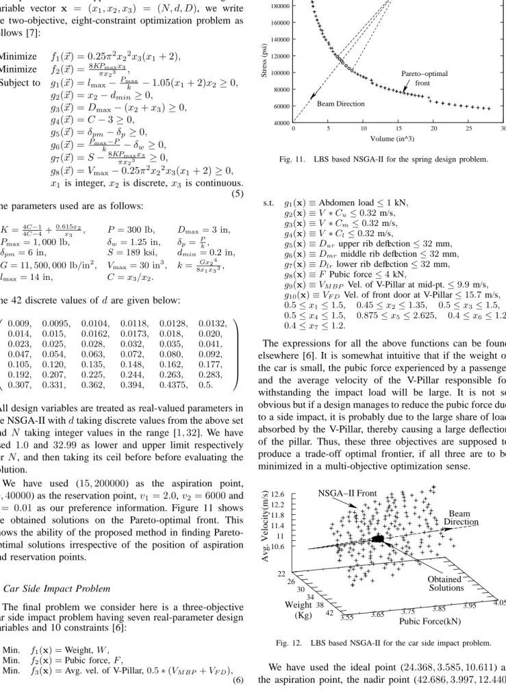
I. Car Side Impact Problem
The final problem we consider here is a three-objective car side impact problem having seven real-parameter design variables and 10 constraints [6]:
Min. f1(x) =Weight,W ,
Min. f2(x) =Pubic force,F ,
Min. f3(x) =Avg. vel. of V-Pillar,0.5∗(VM BP+VF D),
(6) Volume (in^3) Stress (psi) Beam Direction Pareto−optimal front 40000 60000 80000 100000 120000 140000 160000 180000 200000 0 5 10 15 20 25 30
Fig. 11. LBS based NSGA-II for the spring design problem.
s.t. g1(x)≡Abdomen load≤1kN,
g2(x)≡V ∗Cu≤0.32m/s,
g3(x)≡V ∗Cm≤0.32m/s,
g4(x)≡V ∗Cl≤0.32m/s,
g5(x)≡Dur upper rib deflection≤32mm,
g6(x)≡Dmr middle rib deflection≤32mm,
g7(x)≡Dlr lower rib deflection≤32mm,
g8(x)≡F Pubic force≤4kN,
g9(x)≡VM BP Vel. of V-Pillar at mid-pt.≤9.9m/s,
g10(x)≡VF D Vel. of front door at V-Pillar≤15.7m/s,
0.5≤x1≤1.5, 0.45≤x2≤1.35, 0.5≤x3≤1.5,
0.5≤x4≤1.5, 0.875≤x5≤2.625, 0.4≤x6≤1.2,
0.4≤x7≤1.2.
The expressions for all the above functions can be found elsewhere [6]. It is somewhat intuitive that if the weight of the car is small, the pubic force experienced by a passenger and the average velocity of the V-Pillar responsible for withstanding the impact load will be large. It is not so obvious but if a design manages to reduce the pubic force due to a side impact, it is probably due to the large share of load absorbed by the V-Pillar, thereby causing a large deflection of the pillar. Thus, these three objectives are supposed to produce a trade-off optimal frontier, if all three are to be minimized in a multi-objective optimization sense.
Avg. Velocity(m/s) Pubic Force(kN) Weight (Kg) DirectionBeam Solutions Obtained NSGA−II Front 22 26 30 34 38 42 3.55 3.65 3.75 3.85 3.95 4.05 10.6 11 11.4 11.8 12.2 12.6
Fig. 12. LBS based NSGA-II for the car side impact problem.
We have used the ideal point (24.368,3.585,10.611) as the aspiration point, the nadir point (42.686,3.997,12.440)
as the reservation point, v1 = 2.0, v2 = 2.0,v3 = 0.4and
= 0.02. The nadir point is found by using a NSGA-II-based methodology proposed earlier [5]. The solutions obtained on the Pareto-optimal front are as shown in Figure 12.
VI. COMPARISON OFINTERACTIVEEMO METHODOLOGIES
With an increase in attention for developing interactive EMO methodologies, it is also important to know the pros and cons of different strategies. Here, we compare the LBS strategy with the previously suggested reference point and reference direction based EMO methodologies.
• Reference point based EMO [7]: One or more
ref-erence points, a weight vector, for spread are user-supplied. The procedure finds a region close to the Pareto-optimal solution corresponding to the achieve-ment scalarized solution from the reference point. Mul-tiple reference points can be used. The procedure works with more than one reference point simultaneously. Some obtained solutions can be non Pareto-optimal.
• Reference direction based EMO [6]: One or more
reference directions, each dictated by two points on the objective space, a weight vector and number of points on each reference direction are user-supplied. The proce-dure finds a set of Pareto-optimal solutions correspond-ing to reference points along the reference direction. In some sense, the obtained Pareto-optimal solutions are projection of points on a reference direction. Multiple reference directions can be used simultaneously. This method theoretically finds Pareto-optimal solutions.
• Light beam search based EMO (this study): One
or more pairs of aspiration and reservation points, veto threshold vector, are user-supplied. The procedure finds the portion of the Pareto-optimal frontier, in some sense, illuminated by the light beam emanating from the aspiration point towards the reservation point with a span dictated by veto threshold. Multiple light beams can be considered simultaneously. Density of solutions are governed by . This method theoretically finds Pareto-optimal solutions.
Each of the above methodologies finds a set of Pareto-optimal solutions in a preferred region dictated by different parameters. Such a methodology must have to be used iteratively with the help of a utility function or other decision-making aides so that one or more particular solutions can be chosen from the obtained set and a similar EMO procedure can be applied once again. Such an iterative procedure should continue till the DM is satisfied with the obtained solution.
VII. CONCLUSIONS
In this paper, we have used an EMO procedure along with the concept of the light beam search strategy for finding a preferred set of Pareto-optimal solutions. By specifying an aspiration point and a reservation point, the search results in focusing on the Pareto-optimal frontier by a divergent light beam controlled by a veto threshold vector. The distribution
of the solutions in the focussed region is controlled by an parameter. Using the above procedure, the decision-maker can also obtain more than one set of preferred regions simultaneously by simply choosing multiple light beams. Its strength is evident from its ability to converge satisfactorily to the true Pareto-optimal front even for a ten-objective optimization problem. In addition, the suggested procedure has also been able to find a uniformly distributed set of solutions. Upto three objective problems it achieves exactly the true Pareto-optimal solutions, whereas for higher objective problems the obtained solutions are very close to the true Pareto-optimal front. The procedure is now ready to be implemented with a GUI-based procedure so that DM can specify aspiration and reservation points and other parameters interactively and the above procedure can be applied iteratively till a single preferred solution is found.
ACKNOWLEDGEMENT
This study is supported by a gift support by General Motors R&D, Bangalore.
REFERENCES
[1] J. Branke and K. Deb. Integrating user preferences into evolutionary multi-objective optimization. In Y. Jin, editor, Knowledge
Incor-poration in Evolutionary Computation, pages 461–477. Hiedelberg,
Germany: Springer, 2004.
[2] J. Branke, T. Kauβler, and H. Schmeck. Guidance in evolutionary multi-objective optimization. Advances in Engineering Software,
32:499–507, 2001.
[3] K. Deb. Multi-objective optimization using evolutionary algorithms. Chichester, UK: Wiley, 2001.
[4] K. Deb, S. Agrawal, A. Pratap, and T. Meyarivan. A fast and elitist multi-objective genetic algorithm: NSGA-II. IEEE Transactions on
Evolutionary Computation, 6(2):182–197, 2002.
[5] K. Deb and S. Chaudhuri. Towards estimating nadir objective vector using evolutionary approaches. In Proceedings of the Genetic and
Evolutionary Computation Conference (GECCO-2006), pages 643–
650. New York: The Association of Computing Machinery (ACM), 2006.
[6] K. Deb and A. Kumar. Interactive evolutionary multi-objective optimization and decision-making using reference direction method. Technical Report KanGAL report number 2007001, Kanpur Genetic Algorithms Laboratory, Department of Mechanical engineering, Indian Institue of Technology Kanpur, India, 2007.
[7] K. Deb, J. Sundar, N. Uday, and S. Chaudhuri. Reference point based multi-objective optimization using evolutionary algorithms.
In-ternational Journal of Computational Intelligence Research (IJCIR),
2(6):273–286, 2006.
[8] A. Jaszkiewicz and R. Slowinski. The light beam search approach – An overview of methodology and applications. European Journal of
Operation Research, 113:300–314, 1999.
[9] M. Luque, K. Miettinen, P. Eskelinen, and F. Ruiz. Three different ways for incorporating preference information in interactive reference point based methods. Technical Report W-410, Helsinki School of Economics, Helsinki, Finland, 2006.
[10] S. Phelps and M. Koksalan. An interactive evolutionary metaheuristic for multiobjective combinatorial optimization. Management Science, 49(12):1726–1738, December 2003.
[11] L. Thiele, K. Miettinen, P. Korhonen, and J. Molina. A preference-based interactive evolutionary algorithm for multiobjective optimiza-tion. Technical Report Working Paper Number W-412, Helsingin School of Economics, Helsingin Kauppakorkeakoulu, Finland, 2007. [12] A. P. Wierzbicki. The use of reference objectives in multiobjective optimization. In G. Fandel and T. Gal, editors, Multiple Criteria
Decision Making Theory and Applications, pages 468–486. Berlin: