What macroeconomic shocks affect the
German banking system?
Analysis in an integrated micro-macro model
Sven Blank
(University of Tübingen)
Jonas Dovern
(Kiel Institute for the World Economy)
Discussion Paper
Series 2: Banking and Financial Studies
No 15/2009
Editorial Board: Heinz Herrmann
Thilo Liebig
Karl-Heinz Tödter
Deutsche Bundesbank, Wilhelm-Epstein-Strasse 14, 60431 Frankfurt am Main, Postfach 10 06 02, 60006 Frankfurt am Main
Tel +49 69 9566-0
Telex within Germany 41227, telex from abroad 414431 Please address all orders in writing to: Deutsche Bundesbank,
Press and Public Relations Division, at the above address or via fax +49 69 9566-3077 Internet http://www.bundesbank.de
Reproduction permitted only if source is stated. ISBN 978-3–86558–579–0 (Printversion) ISBN 978-3–86558–580–6 (Internetversion)
Abstract
We analyze what macroeconomic shocks affect the soundness of the German bank-ing system and how this, in turn, feeds back into the macroeconomic environment. Recent turmoils on the international financial markets have shown very clearly that assessing the degree to which banks are vulnerable to macroeconomic shocks is of utmost importance to investors and policy makers. We propose to use a VAR framework that takes feedback effects between the financial sector and the macroe-conomic environment into account. We identify responses of a distress indicator for the German banking system to a battery of different structural shocks. We find that monetary policy shocks, fiscal policy shocks, and real estate price shocks have a significant impact on the probability of distress in the banking system. We identify some differences across type of banks and different distress categories, though these differences are often small and do not show any systematic patterns.
Keywords: VAR, banking sector stability, sign restriction approach
Non-technical summary
To understand how the financial system is influenced by macroeconomic shocks and how the financial stance of the economy in turn feeds back into the macroe-conomic environment is key for policy makers. In this paper, we analyze how different macroeconomic shocks affect the German banking system.
To this end, we draw on a micro-macro stress-testing framework for the Ger-man banking system that has recently been proposed by De Graeve et al. (2008). The micro-level explains the distress probabilities of banks. The macro-level is described by a vector autoregressive (VAR) model. The two appealing features of this approach are, on the one hand, that it makes use of both, macro and bank-specific data and, on the other hand, that it allows for contemporaneous feedback effects between the macro- and micro-level.
Formally, we augment the baseline version of the integrated micro-macro model by a set of additional endogenous variables and a set of additional exogenous variables in the VAR. By extending the model in this way, it becomes feasible to identify fiscal shocks (Caldara and Kamps, 2008), exchange rate, and asset price shocks (Fratzscher et al., 2007).
To identify structural shocks from the reduced form VAR, restrictions have to be imposed. Like De Graeve et al. (2008), the approach recently proposed by Uhlig (2005) is followed, which achieves identification of the VAR by imposing sign-restrictions on the impulse responses of a set of variables. The main advantage of this identification scheme is that only relative mild identifying assumptions have to be made. For instance, the results are insensitive to the ordering of the variables in the VAR. Thus, we do not have to take any stance on how the banking sector should respond to a particular shock. Instead, the data can speak freely about the effects of the shocks on the banking sector.
The empirical results lead to the following conclusions. First, there is a close link between macroeconomic developments and the stance of the banking sector. Second, monetary policy shocks are the most influential shocks for the develop-ment of the distress indicator. Third, fiscal policy shocks and real estate price shocks have a significant impact on the distress indicator. However, the evidence is mixed for exchange rate shocks. Equity price shocks have no impact at all. Fourth, for the identification of most shocks it is essential to work in the inte-grated model that combines the micro and the macro evidence.
The scarce availability of data for the banking sector that is used to estimate the micro level of the integrated model makes an estimation of a “global” model, that includes all relevant variables altogether, infeasible. However, it would be very interesting to address this issue in future work with an extended data set.
Nicht-technische Zusammenfassung
Wie der Finanzsektor von makro¨okonomischen Schocks beeinflusst wird und wie dies wiederum auf das makro¨okonomische Umfeld wirkt, ist von zentraler Bedeu-tung f¨ur Wirtschaftspolitiker. In diesem Papier untersuchen wir die Auswirkungen verschiedener makro¨okonomischer Schockszenarien auf das deutsche Bankensys-tem.
Zu diesem Zweck greifen wir auf ein Mikro-Makro-Stress-Testing Modell zur¨uck, das von De Graeve et al. (2008) entwickelt wurde. Auf der Mikroebene erkl¨aren wir die Wahrscheinlichkeit einer Schieflage von Banken; auf der Makroebene modellieren wir ein vektorautoregressives Modell (VAR). Die zwei wichtigsten Vorteile des verwendeten Ansatzes sind, dass er sowohl Informationen aus makro-¨
okonomischen Daten als auch aus mikro¨okonomischen, bankspezifischen Daten ber¨ucksichtigt und dass das Modell kontempor¨are R¨uckkoppelungseffekte zwis-chen Makro- und Mikroebene zul¨asst.
Wir erweitern die Grundversion des integrierten Mikro-Makro-Modells durch zus¨atzliche endogene und exogene Variablen im VAR-Modell. Diese Erweiterung erm¨oglicht es, mehr fundamentale Schocks zu indentifizieren, wie z.B. fiskalpoli-tische Schocks (Caldara and Kamps, 2008) oder Wechselkurs- und Aktienpreis-schocks (Fratzscher et al., 2007).
Wie De Graeve et al. (2008) nutzen wir den von Uhlig (2005) vorgeschlagenen Sign-Restriction-Ansatz, um von der Sch¨atzung der reduzieren Form des VAR-Modells auf die Wirkung der strukturellen Schocks zu schließen. Der Vorteil dieser Methode ist, dass nur relativ milde Annahmen bez¨uglich aufzuerlegender Restrik-tionen getroffen werden m¨ussen. Die Ergebnisse sind zum Beispiel nicht sensitiv hinsichtlich der Ordnung der Variablen im VAR-Modell. Der Ansatz erm¨oglicht es uns, keine Annahmen ¨uber die kontempor¨are Reaktion des Bankensektors auf makro¨okonomische Schocks treffen zu m¨ussen, sondern die dynamischen Reak-tionsmuster ausschließlich aus den Daten zu sch¨atzen.
Unsere empirischen Ergebnisse lassen folgenden Schlussfolgerungen zu. Er-stens best¨atigen die Sch¨atzungen, dass ein enger Zusammenhang zwischen makro-¨
okonomischen Entwicklungen und dem Zustand des Bankensektors besteht. Zweit-ens sind geldpolitische Schocks mit Abstand die einflussreichsten Schocks f¨ur den Zustand des Bankensektors. Drittens haben Fiskalschocks und Immobilienpreiss-chocks einen Einfluss auf den Zustand des Bankensektors, w¨ahrend die Evidenz
hinsichtlich der Effekte von Wechselkursschocks gemischt ist. Außerdem zeigen die Ergebnisse, dass Schocks auf Aktienpreise keinen Einfluss auf den Zustand des Bankensystems haben. Viertens ist es f¨ur die Identifizierung der meisten Schocks essenziell mit dem kombinierten Modell zu arbeiten, welches sowohl die Mikro-als auch die Makroebene integriert.
Die geringe Verf¨ugbarkeit an Bankdaten, die zur Sch¨atzung der Mikroebene des integrierten Modells herangezogen werden, macht die Sch¨atzung eines “glob-alen” Modells, das alle relevanten Variablen integriert, unm¨oglich. Es w¨are sehr in-teressant ein solches Modell mit einem erweiterten Datensatz in einer zuk¨unftigen Arbeit zu analysieren.
Contents
1 Introduction 1
2 The Model 4
2.1 The Basic Model . . . 4
2.2 Extending the Basic Model . . . 6
2.3 Identification of Structural Shocks . . . 6
3 Data 7 3.1 Data Sources . . . 7 3.2 Data Availability . . . 9 4 Stylized Facts 9 5 Results 10 5.1 Micro-Level Estimates . . . 10
5.2 Responses to Macroeconomic Shocks in the Combined Framework 14
6 Conclusion 17
List of Figures
1 Distress Indicator and Macroeconomic Variables . . . 28
2 Monetary Policy Shock in the Integrated VAR . . . 28
3 Aggregate Demand Shock in the Integrated VAR . . . 29
4 Aggregate Supply Shock in the Integrated VAR . . . 29
5 Equity Price Shock in the Integrated VAR . . . 30
6 Pure Government Revenue Shock in the Integrated VAR . . . 30
7 Contractionary Fiscal Policy Shock in the Integrated VAR . . . . 31
8 Real Estate Price Shock in the Pure Macro VAR . . . 31
9 Real Estate Prices Shock in the Integrated VAR . . . 32
10 Exchange Rate Shock in the Integrated VAR . . . 32
11 Exchange Rate Shock in the Integrated VAR (longer restrictions) 33
List of Tables
1 Cross-Correlations . . . 222 Analyzed Shocks and Corresponding Models . . . 22
3 Micro-Level Estimations for Baseline Scenario . . . 23
4 Micro-Level Estimations with German Stock Market Index . . . . 24
5 Micro-Level Estimations with Fiscal Variables . . . 25
6 Micro-Level Estimations with Real Estate Prices . . . 26
What Macroeconomic Shocks Affect the German Banking
System? Analysis in an Integrated Micro-Macro Model
*1
Introduction
We analyze what macroeconomic shocks affect the soundness of the German bank-ing system and how this, in turn, feeds back into the macroeconomic environment. Recent turmoils on the international financial markets have shown very clearly that continuously monitoring the banking system and quantifying the risks to which banks are exposed is of utmost importance to investors and policy makers. Over the last two decades, stress testing at the level of financial institutions has be-come more and more important in addition to traditional approaches like value-at-risk (VaR) (Committee on the Global Financial System, 2001). However, stress testing from a macroeconomic perspective has attracted attention not until more recent years (Sorge, 2004).
In this paper, we demonstrate how the recently introduced approach by De Graeve et al. (2008) can be extended to allow for identification of a richer va-riety of macroeconomic shocks. Their approach combines the micro (banks) and macro (entire economy) sphere into an integrated model framework for analyzing the sensitivity of the banking sector to macroeconomic shocks. The two appealing features of this approach are, on the one hand, that it makes use of both macro and bank-specific data and, on the other hand, that it allows for contemporaneous feedback effects between the macro and micro level in both directions. Both fea-tures are also advantageous when analyzing shocks different to the ones presented in De Graeve et al. (2008).
Motivated by the financial crises in emerging markets in the late 1990’s and the increasing world wide integration of financial markets, central banks and
in-*Sven Blank, University of T¨ubingen, [email protected]; Jonas Dovern, The
Kiel Institute for the World Economy (IfW),[email protected]. Financial support
by “Stiftung Geld und W¨ahrung” is highly appreciated by both authors. The authors would like
to thank the banking supervision department of the Deutsche Bundesbank for its hospitality and for access to its bank-level data. We would also like to thank Claudia Buch, Ferre De Graeve, Thomas Kick, Michael Koetter and Thomas Laubach for very helpful comments. Any errors are of course the responsibility of the authors. The views presented in this paper reflect the authors’ opinion, and do not necessarily coincide with those of the IfW or the Deutsche Bundesbank.
ternational institutions took lead in augmenting the micro perspective at the individual bank by a macro perspective that addresses overall financial stability. Even though the weakness of individual banks possibly will be the trigger to larger crises, it is mostly the deterioration of macroeconomic environment that makes the single bank fail and may cause chain reactions in a tightened surrounding (Gavin and Hausmann, 1996). Major crises in the financial system, therefore, cannot simply be dispatched as a result of failures in single institutions. It is the interaction between the financial system and the macro-economy that drives the dynamics. Increasingly, central banks and international organizations study this interaction to assess the resilience of the financial system – especially the banking sector – to extreme but plausible shocks to its operational environment (European Central Bank, 2006). The most extensive appliance of macroeconomic stress testing so far has been accomplished by the IMF as part of its Financial System Assessment Programs (FSAPs).1
Existing evidence on feedback effects between the real economy and the finan-cial sector suggests that the link between the two parts of the De Graeve et al. (2008) model is indeed very important (Goodhart et al., 2004, 2006). On the one hand, the well-being of the banking sector – as measured by various balance sheet items – can be affected by macroeconomic shocks (see e.g. Dovern et al., 2008). On the other hand transmission channels are also working in the oppo-site direction; the two most important concepts are thebank lending channel and the financial accelerator effect. The former concerns the intermediation role of banks in transmitting changes in the monetary policy stance into the real econ-omy (see e.g. Bernanke and Gertler, 1989). The second effect refers to the fact that frictions in the banking sector can amplify business cycle fluctuations (see e.g. Kiyotaki and Moore, 1997, Bernanke et al., 1999, Allen and Saunders, 2004). While we do not identify the contribution of each channel to the shock transmis-sion in our empirical analysis below, the integrated micro-macro framework in principle allows both channels to be prevalent.
The basic model by De Graeve et al. (2008) has been extended recently along several dimensions. De Graeve and Koetter (2007a) expand the model to allow for endogenous balance sheet adjustments in the banking sector in response to macroeconomic shocks by making the bank specific variables in the baseline model react endogenously to variations in the other variables. They show that only the
share of customer loans reacts significantly to monetary policy shocks while the other bank specific variables are not affected. De Graeve and Koetter (2007b) propose an identification scheme that can be used to identify an exogenous fi-nancial distress shock in the extended model. They show that while the effects of monetary policy and aggregate supply shocks remain the same, those effects attributed to aggregate demand shocks in the original model are likely to actually reflect the influence of financial distress shocks.
The original model is extended by Blank et al. (2009) along a different dimen-sion. The authors explore whether shocks originating at large banks affect the probability of distress of smaller banks. To this end, they construct a measure of idiosyncratic shocks at large banks and include this measure into the integrated model proposed by De Graeve et al. (2008). They conclude that positive shocks at the large banks reduce the probability of distress for smaller banks.
In this paper, we extend the model along a third dimension. While the con-tributions mentioned so far made an attempt to introduce more realistic features into the micro part of the integrated model, we enlarge the macro part of the model. By doing so, we are able to identify additional macroeconomic structural shocks which might be of interest in stress testing the banking system.
Our results support the following conclusions. First, the results show a close link between macroeconomic developments and the stance of the banking sector. We find some differences across sub-samples by restricting the data for estimation to only those observations that corresponds to a certain category of distress events or to certain types of banks. There is a larger impact of macroeconomic variables for weaker distress events. In addition, the results are more robust for cooperative banks. Second, monetary policy shocks are the most influential shocks for the de-velopment of the distress indicator. Third, while also fiscal policy shocks and real estate price shocks have a significant impact on the distress indicator. However, the evidence is mixed for exchange rate shocks. For equity price shocks we do not find any impact. Fourth, for the identification of most shocks it is essential to work in the integrated model that combines micro and macro evidence.
The remainder of the paper is structured as follows. In Section 2, we present the model framework in which we analyze the stability of the banking sector. We show how the reduced form integrated micro-macro VAR model is extended to allow for a richer set of structural shocks and how we identify these shocks. In Section3, we briefly outline the different data sets which are used in the empirical
analysis. In Section 4, we show some basic correlation statistics to demonstrate how our indicator of financial distress moves in line with several macroeconomic variables. In Section 5, we present the empirical results of our analysis. We present results for the microeconomic model as well as for the combined approach for the full sample and various sub-samples of our data. Section 6 concludes the paper.
2
The Model
2.1
The Basic Model
The basic model is presented in De Graeve et al. (2008). Their extension of an approach proposed by Jacobson et al. (2005) combines macroeconomic and indi-vidual data on single banks in one integrated model framework that allows for feedback effects between micro and macro data in both directions. The microe-conometric part of the model is given by a binary model that links the probability of distress (P D) for a bank to bank specific covariates and macroeconomic vari-ables. The macroeconometric part is modeled as a vector autoregressive (VAR) model including the most important macroeconomic variables. As shown below the two parts are combined to yield an integrated VAR model that inherits all features described so far.
The key equation at the micro-level explains a bank’s P D as a function ofk1 bank specific covariates, collected in vector Xit, andk2 macroeconomic variables, collected in vector Zt:
P Dit=
exp(β1Xit−1+β2Zt−1)
1 + exp(β1Xit−1+β2Zt−1) (1) This equation is estimated using yearly data and a pooled logit model.2 Since we expect the explanatory variables to have a delayed impact on the probability of a distress event of a bank, we adopt the specification proposed by De Graeve et al. (2008) and choose a lag length of one year which is suggested by conventional lag selection criteria.
2Note that the macroeconomic variables do not vary across the different banks. Hence, we
cannot include time fixed effects in the regressions. As a consequence, the marginal effects of the macroeconomic variables potentially reflect to some degree the effects of unobserved macroeconomic factors.
The macro part of the model can be written as
Zt = ΠMMZt−1+ ΠF MP Dta−1+ut. (2)
It models the dynamics of the macroeconomy as an autoregressive process of Zt. As an additional explanatory variable we include the aggregate probability of bank distress, P Dat, which is constructed as in De Graeve et al. (2008) and measured by the frequency of distressed events across all banks in the sample.
The VAR approach is used for three reasons. First, VARs usually perform relatively well in describing the data generating process of macroeconomic vari-ables. Second, the general form of the model is not based on any structural assumptions on the way financial distress and the macroeconomy interact. A con-sensus on the effectiveness of different transmission channels has not yet emerged (European Central Bank, 2005). It is therefore appealing to resort to a model that needs as little a priori theorizing as possible. Finally, the structure of the model allows us to introduce feedback effects in a very convenient way in the next step.
Note that so far the model does not incorporate the feedback effects between the micro and the macro sphere, since P Dta is assumed to be exogenously deter-mined. To obtain the integrated model, we need to augment the macroecono-metric model by one equation originating from the micro part that describes the evolution of the probability of distress.
Zt P Da t = ΠMM ΠMF Zt−1 + ΠF M ΠF F P Da t−1+t (3)
The elasticity of the probability of distress with respect to the macroeconomic variables is given by the outcome from the microeconometric part of the model:
ΠMF ≡∂P(P Dit= 1|Zt−1, Xit−1)
∂Zt
= exp( ˆβ1Xit−1+ ˆβ2Zt−1) 1 + exp( ˆβ1Xit−1+ ˆβ2Zt−1)
2 βˆ2 (4)
Note that by imposing the estimated effects from the microeconometric model the bank specific variables retain an important role in the integrated model although they are assumed to be exogenous at this stage. This is because ΠMF depends on the level of each of the variables in the micro part of the model.3
3De Graeve et al. (2008) note that this feature makes the coefficients state dependent and
2.2
Extending the Basic Model
In this subsection, we enhance the basic model by ? to allow for a wider set of macroeconomic shocks. We can write an augmented version of the model presented in Equation (3) as
Yt= ΠYt−1+ ΓWt+t, (5)
where Yt = [ZtP Dtay1y2 . . . yp] includes the endogenous variables of the basic model together with p additional endogenous variables, Wt = [w1w2 . . . wq] de-notes a vector of q exogenous variables, and Π and Γ are properly dimensioned coefficient matrices. By extending the model with the appropriate additional ex-ogenous and endex-ogenous variables it becomes feasible to identify more specific fundamental shocks – such as fiscal shocks (Caldara and Kamps, 2008), or ex-change rate and asset price shocks (Fratzscher et al., 2007) – than in the basic model where the variation could only be attributed to monetary policy shocks, aggregate supply shocks, or aggregate demand shocks (De Graeve et al., 2008).
2.3
Identification of Structural Shocks
Starting from the complete reduced form n-dimensional VAR given in Equation (5), we are interested in the responses of the variables in Yt to various structural shocks. To this end, the vector of prediction errorsut has to be translated into a vector of economically meaningful structural innovations. The essential assump-tion in this context is that these structural innovaassump-tions are orthogonal to each other. Consequently, identification amounts to providing enough restrictions to uniquely solve for a decomposition of the covariance matrix of the reduced form VAR: Σ =A0A0. This defines a one-to-one mapping from the vector of orthogo-nal structural shocks νt to the reduced-form residuals, ut=A0νt. Because of the orthogonality assumption, and the symmetry of Σ, only n(n−1)/2 restrictions need to be imposed to pin downA0.
Like De Graeve et al. (2008), we follow an approach recently proposed by Uhlig (2005), which achieves identification of the VAR by imposing sign-restrictions on
variables. While we do not pursue this issue in this paper and set ΠMF equal to its value obtained
for the sample averages ofXitandZt, an example of such an analysis can be found in the paper
the impulse responses of a set of variables.4 Identification of the model is achieved by a simulation approach.5
This so-called “pure sign-restriction approach” has one main advantage. Sign-restrictions are relative mild identifying assumptions compared to conventional approaches like identification through recursive ordering of the variables or long-run zero restrictions. The obtained results are, for instance, insensitive to the specific decomposition of Σ or the ordering of the variables in the VAR.6 Thus, we do not have to take any stance on how the banking sector should respond to a particular shock. Instead, we let the data speak about the effects of the shocks on the banking sector.
3
Data
3.1
Data Sources
3.1.1 Distress Indicators
For the estimation of the micro part of the model, we use data on distress events among German banks between 1994 and 2004 from the annual distress database of the Deutsche Bundesbank. These data are confidential and are available on the premises of the Deutsche Bundesbank only. The construction of the distress events follows the classification proposed by Kick and Koetter (2007) and used by De Graeve et al. (2008).7 The data includes the following four categories of distress events. The weakest type of distress (”distress category I”) comprises mandatory announcements by individual banks to the supervisory authority like a drop of annual operational profits or liable capital by more than 25%. The second category (”distress category II”) captures official warnings by the German
4Initially it has been proposed to obtain these restrictions by choosingA
0to be a Cholesky
factorization of Σ, implying a recursive ordering of the variables as in Sims (1986). This
method has been questioned on various grounds (see e.g. Sims, 1992, Grilli and Roubini, 1996, Christiano et al., 1998). Although, alternative identification schemes like for instance the ap-proach proposed by Blanchard and Quah (1989) have been introduced in the past, none of them has remained without criticism (Fernald, 2007).
5For the specifics of this Bayesian estimation strategy we refer to Appendix B in Uhlig (2005).
6De Graeve et al. (2008) note that in fact for some standard identifying restrictions like for
instance for a monetary policy shock, “the restrictions [in the sign-restriction approach] nest the recursive (or Choleski) response.”
financial supervisory authority (Bundesanstalt f¨ur Finanzdienstleistungsaufsicht,
BaFin). A more severe sign of banking distress (”distress category III”) are direct interventions into the ongoing business of a bank by the BaFin, like restrictions to lending or deposit taking. In addition, this category also comprises capital injections by the insurance scheme of the respective banking sector. Finally, the worst distress category (”distress category IV”) comprises all closures of banks and restructuring mergers.
On the aggregate level, the probability of distress is constructed as the ratio of distress events in the banking sector to the total number of banks in the sample. It measures the unconditional frequency of distress events across the banking sector.8
3.1.2 Other Bank-Specific Variables
Information on individual bank balance sheets comes from confidential data col-lected by theDeutsche Bundesbank. Since the number of bank-specific covariates is potentially very large, we use a selection of variables that have been identified by De Graeve et al. (2008) following an approach by Hosmer and Lemeshow (2000). The selection procedure is oriented at the so-called CAMEL (Capitalization, As-set quality, Management, Earnings, and Liquidity) taxonomy (King et al., 2006). Details on the selection process can be found in the paper by De Graeve et al. (2008). The bank-specific variables which are taken into account, are the eq-uity ratio, total reserves, customer loans, off-balance sheet activities, size, return on equity and liquidity. Consequently, the vectors Xit contains eight variables (including a constant).
3.1.3 Macroeconomic Variables
The set of variables representing the macroeconomy consist of the three stan-dard variables, namely GDP growth, consumer price inflation, and the short term interest rate; consequently, the vector Zt has dimension three. In the different augmented models that we show in the next section, we include the German stock market index (DAX-index), government revenues and expenditures, a price defla-tor for construction in the housing secdefla-tor (which serves as a proxy for real estate
8Three subset databases of the distress database (measures, incidents, distressed mergers),
which contain information about exact dates, are used to allocate the distress events to quarters to construct this series on a quarterly frequency; this is done to match the highest frequency available for the macroeconomic variables described below.
prices), and the nominal effective exchange rate, respectively. The data – except for the exchange rate and the interest rate – have been seasonally adjusted prior to differencing.
3.2
Data Availability
The sample period is restricted by the availability of bank specific data on distress events and the banks’ characteristics. In its currently available form, these data cover the period from 1994 to 2004. We use annual data to estimate the model in Equation (1) since the properties of the data on the bank specific covariates do not allow to switch to a higher frequency. Due to the panel structure of the data with a fairly high cross-section dimension, estimation is feasible with effectively ten years of data.
The sample for the macroeconomic variables is chosen correspondingly. To enable us to estimate versions of the extended model given in Equation (5) we use quarterly data and transform the estimates subsequently to conform with the microeconometric part. Still, the sample size is relatively low and does not allow for estimation of very rich models, i.e. q andpcannot be chosen to be large. This is why estimation of a universal model is infeasible.
4
Stylized Facts
Before we present our model and the results of our formal econometric analysis, we give some stylized facts about the relation between the soundness of the banking system and the macroeconomy in this section.
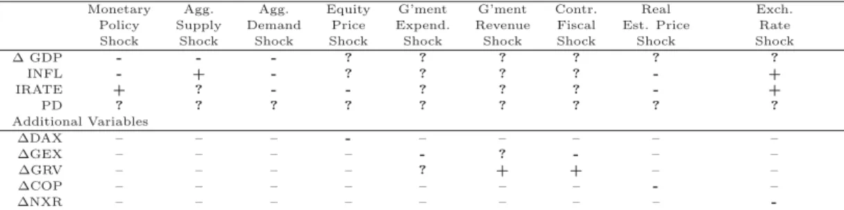
The distress indicator shows a substantial degree of co-movement with most of the macroeconomic variables (Figure 1). It seems to be especially moving to-gether with GDP growth, stock return, change of government expenditure, and the exchange rate. This visual impression is supported by an analysis of correla-tion coefficients which shows that the distress indicator is substantially negatively correlated to those six variables (Table1). There are differences, however, in the size of the correlation and the lag at which a high correlation can be found.
The distress indicator shows a strong contemporaneous correlation with GDP growth and stock returns, that is strong growth and high stock market returns go in line with a reduction of the probability of distress events in the banking
sector. In contrast, the distress indicator seems to lag behind the development of government expenditures and, even more pronounced, the exchange rate, i.e. increases of government expenditure and an appreciation of the Euro are followed by a reduction of the probability of distress events in the banking sector.
Hence, there seems to be indeed some interaction of the stance of the banking system and macroeconomic factors. This in turn indicates that the identification of structural shocks is of particular importance. To analyze which shocks exactly drive this interaction, we have to move to a formal econometric model.
5
Results
5.1
Micro-Level Estimates
On the micro level we estimate the impact of our bank-specific covariates and macroeconomic variables on the probability of distress using the model that is given by Equation 1. The results are given in the appendix (Tables 3to 7).
5.1.1 Results for the Full Sample
In the baseline model (Table 3, column (1)), the estimates of the marginal ef-fects of bank-level and macro-level variables largely confirm the results shown in De Graeve et al. (2008). The explanatory power, as measured by the pseudo-R2 is 11.45 %.
Better capitalized banks, i.e. banks with a higher equity ratio and higher reserves, have a lower probability of distress. The coefficients are negative and highly significant. Higher customer loans and broader off-balance sheet activities imply higher credit risk, and we would expect a positive impact on the probability of distress (Kick and Koetter, 2007). While we find the influence of off-balance sheet activities to be insignificant, this is indeed the case for customer loans. The size of small and medium-sized banks significantly reduces the likelihood of a distress event. In addition, more profitable banks, as measured by the return on equity, have a lower probability of distress. One could argue that banks with higher liquidity are less likely to experience a distress event. On the other hand, liquidity is consistent with a ’signaling effect’. High liquidity signals a lack of interest-bearing investment possibilities and thus low profitability. In fact, similar to Blank et al. (2009), we find this signaling effect to dominate, since liquidity
enters positively significant.
A positive macroeconomic environment, as measured by higher real GDP growth, that is usually accompanied by rising prices, should reduce the proba-bility of distress. We find indeed a significantly negative coefficient for both, real GDP growth as well as inflation for most of the sub-samples. We would expect the interest rate to exert a positive influence on the probability of distress as it higher costs of refinancing. However, in the baseline scenario, the interest rate is insignificant.
The remaining models allow for a more comprehensive impact of the macroeco-nomic environment on the probability of distress. The estimates show that adding additional macroeconomic variables to this baseline specification leaves the result for the bank-specific covariates remarkably stable in general.
In Table4column (1), we report our results for the effects of a change in stock market valuation. A rise of the DAX has a significant negative impact on the probability of distress. Some of the effect might be due to the signaling property of the DAX for business cycle movements. But there could also exist a direct effect since banks hold some of their assets in equity which leads to re-valuations of the banks’ assets due to changes in stock prices. This might – in case of an adverse shock – lead to an increasing distress probability. The coefficients for the other three macroeconomic variables remain unchanged.
In Table 5 column (1), we report our results for fiscal policy effects. In this model, we also include dummies to account for the extraordinary high revenues through alienation of UMTS licences in 2000. Government revenues have a sig-nificant positive effect on banks’ probability of distress, whereas expenditures are insignificant. The positive sign for revenues may be explained by higher tax bur-den that might increase the likelihood of borrowers’ defaults. In addition, we find, somewhat unexpectedly, a negative coefficient for the interest rate.
In Table 6 column (1), we report our results for the effects of changes on the real estate market. Like increasing inflation, rising prices for construction in the housing sector should reduce the probability of distress. Indeed, we find a negative significant effect in both specifications. Also, the interest rate now has the expected positive sign.
In Table 7 column (1), we report our results for the effects of exchange rate movements. Roughly 50% of German banks’ foreign liabilities and 30% to 40% of banks’ foreign assets were denominated in foreign currency in the period under
study (see Bank for International Settlements, various years). Thus, an appreci-ation of the Euro should have a significant negative effect on banks’ cross-border assets and liabilities. However, since the ratio of foreign liabilities to foreign assets ranges from 1.1 to 0.7, the impact of valuation changes stemming from exchange rate fluctuations and their effect on the probability of distress is not clear cut. In fact, we find the marginal impact of changes in the nominal effective exchange rate to be insignificant.
5.1.2 Results for Different Distress Categories
So far, we have not accounted for the ordinal character of our endogenous variable. We check the robustness of our results by splitting our sample according to the different categories of distress (see also De Graeve et al., 2008).9 It is likely that the different distress events correlate differently with macroeconomic shocks. One could expect for instance that the weaker distress events as automatic signals or warnings by the financial supervisor, as summarized in categories I and II, are driven by both, bank-specific characteristics as well macroeconomic factors, while severer events are caused solely by bank-specific factors.
The estimation results for the various sub-samples are given in Tables 3 to 7
in columns (2) to (5). In the baseline model without any additional macroeco-nomic variables (Table 3), we indeed find that, together with most bank-specific covariates, GDP growth and inflation enter significantly for distress category I and II. In addition, the interest rate enters significantly positive in the sub-sample for distress category I. In contrast, there is no impact from the macro sphere when considering events that comprise interventions from the banking pil-lars head institution or the financial supervisor into the active business of a bank (distress category III). However, in the most severe distress category, we find a significant impact of inflation and, somewhat weaker, of GDP growth. Thus, the timing of restructuring mergers is influenced by the macroeconomic environment (Blank et al., 2009).
We also check whether these results are in line with the specifications including other macroeconomic factors. The most striking results are given for the model including fiscal variables (Table 5). For the distress category II, the results are very similar to the full sample results. For distress categories I, both, government
9Alternatively, we could also adopt the method employed by Kick and Koetter (2007) and
expenditures and revenues are insignificant. The only macroeconomic factor that drives the likelihood to observe an event assigned to distress category III is gov-ernment expenditures, which enters with a positive sign. One explanation might be that the government could try to stimulate the economy when there is a wors-ening of the business cycle. Hence, an increase in government expenditures could be an indication for a severe recession that increases the probability of distress.
5.1.3 Results for Different Banking Sectors
Next, we check the robustness of our findings if we split up the sample according to Germany’s three banking pillars into private commercial banks, savings banks, and cooperative banks. As the business models of the different types of banks in Germany differ considerably, it is reasonable to expect the different types of banks to be affected differently by certain macroeconomic shocks. For example, cooperative banks may be less exposed to international shocks, since these banks are mainly engaged on the domestic market. We report the detailed results in the appendix in Tables 3 to7, columns (6) to (8).
In the baseline regressions without any additional macroeconomic variables, some of the bank-specific variables as well the macroeconomic aggregates are in-significant. We find the most stable results for cooperative banks, which drive the results for the full sample, as these banks make up nearly 20,000 observations (out of roughly 28,000 observations in the full sample). However, the impact of the size of a bank now switches in sign from being negative to positive. The sub-sample for savings banks comprises approximately 6,000 observations. The only signifi-cant influence from the macroeconomic environment is given by the inflation rate, which enters negatively. In addition to inflation, the interest rate is significant with the expected positive sign if we restrict the sample to private banks, which make up nearly 1,700 observations. Most of the banks-specific covariates turn out to be insignificant in this specification.
For the specifications with an enriched macroeconomic environment, the find-ings compared to the baseline regressions are more or less the same. However, some differences are noteworthy. House prices have a negative significant influ-ence on the probability of distress in the sub-sample for cooperatives as well as in the sub-sample for savings banks. This may be due to the fact that lending on mortgages is more important for these banking sectors than for commercial banks. Government expenditures are positively significant for the sub-sample
comprising savings banks. Government revenues enter positively significant in the sub-sample with cooperative banks. However, the inflation rate now has a positive sign, thus increases the probability of distress. Although the influence of the nominal exchange rate is insignificant for the full sample and for the different distress categories, we find a negative significant impact for both, the sub-sample for the private banks and for the savings banks. We cannot find a significant im-pact for cooperative banks, which are more concentrated on the national economy and, thus, are less prone to valuation effects through exchange rate changes.
5.2
Responses to Macroeconomic Shocks in the Combined
Framework
Having established the impact of the bank-specific and the macroeconomic vari-ables on the micro-level, we pursue and estimate the response of the probability of distress in the VAR framework described in Section 3.2. We do this for both, the pure macro VAR that does not incorporate feedback effects from the macro sphere to the financial sector as well as for the integrated model that allows for mutual macro-micro linkages. We also analyze the response of the financial stance to structural macroeconomic shocks in the various sub-samples. Since the number of scenarios that we study is large, we report only a collection of our results. As mentioned already in Section3.2, we have to use different versions of the extended model that include different sets of additional variables due to the low degrees of freedom. Table 2 gives an overview over the different shocks that we analyze and states which additional variables we include in each case as well as which sign-restrictions are used to identify the shocks.10
5.2.1 Standard Shocks in Baseline Model
As a benchmark, we replicate the findings by De Graeve et al. (2008) in the base-line model without any additional macroeconomic variables. To this end, we analyze the response of the probability of distress to a monetary policy shock. In Figure 2 we show the impulse responses for the combined system. A con-tractionary monetary policy, as given by a rise in the interest rate, significantly
10In setting the identification restrictions, we mainly follow various approaches presented in
the literature – among others by Uhlig (2005), Caldara and Kamps (2008), or Fratzscher et al. (2007).
increases the aggregate probability of distress from the first year onward, pointing to a potential conflict of objectives between the financial supervisor and the Eu-ropean Central Bank. Note that like De Graeve et al. (2008) or Jacobson et al. (2005), we find that integrating the micro part of the model is very important for the dynamics. Neglecting the impact of bank-specific variables leads to consider-able different responses for the probability of distress. To check if these results are robust across different sub-samples or whether we can observe some differences across sub-samples, we split the sample and redo the impulse response analysis. We find similar results for distress category IV. In addition, the response of the probability of distress is very pronounced when restricting the sample to private banks. This may reflect the fact that in contrast to savings banks or cooperative banks those banks rely much more on re-financing via the capital market (as their deposit business is relatively small) and are, hence, directly affected by a change of the yield curve that is usually implied by changes in the short term interest rate.
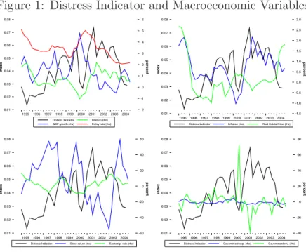
In addition to monetary policy shocks, the baseline model allows to identify aggregate demand and aggregate supply shocks. We find that while an aggregate demand shock causes the distress probability to rise (Figure3), an aggregate sup-ply shock does not seem to have any significant impact on the distress probability (Figure 4). An analysis of sub-samples reveals that the distress probability of savings banks is less affected by aggregate demand shocks - and the effect is only marginally significant. The distress probability of commercial banks is affected -but only for one year after the shock hit the economy. The aggregate result seems to be solely driven by the response of cooperative banks for which the reaction of the distress probability looks like the one for the entire sample. Regarding the aggregate supply shocks, our results show that they have no significant impact for all of the sub-samples.
We now turn to the augmented models that allow us to identify a bunch of other structural shocks in addition to the three basic macroeconomic shocks for which we have presented results so far.11
11Note that we will do not attribute shares of the variation of the distress probability to
specific shocks, since we do not identify all shocks in one model; consequently we cannot perform a forecast error decomposition that takes into account all structural shocks.
5.2.2 Equity Price Shocks
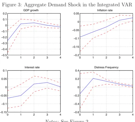
Next, we examine the consequences of an equity price shock. Note that this shock can be understood as a combination of a immediate shock to the banks’ balance sheets (because some of their assets are equity investments) and a more precisely defined aggregate demand shock. The difference to the standard aggregate de-mand shock presented above is simply that we do not force aggregate output to fall but set the sign-restriction in such a way that we specify a specific cause for declining aggregate demand. As Figure 5 shows, we cannot find any signifi-cant impact on the probability of distress. This finding is neither reversed in the integrated model nor for any of the sub-sample estimations.
5.2.3 Fiscal Policy Shocks
When we impose sign-restrictions to identify different fiscal policy shocks, the re-sults depend to a high degree on how the fiscal policy shock is designed. While a “pure government spending shock” (Caldara and Kamps, 2008) does not signif-icantly affect the distress probability even in the integrated model, the opposite is true for a “pure government revenue shock” (Figure 6). A rise in government revenues leads to a significant increase of the distress probability after one year. An explanation is that an increased tax burden leads to a higher insolvency rate among debtors that eventually causes the frequency of distressed events to go up. A weaker, but still significant impact can be found for the sub-sample for cooperative banks as well as distress category II.
Instead of concentrating on just one side of the government budget, one could also argue that what we will call a “contractionary fiscal shock” should be identi-fied by decreasing government expenditures and increasing government revenues. We find that such an identification scheme has a pronounced influence on the dis-tress probability in the integrated model (Figure7). The aggregate probability of distress sharply and significantly increases one period period after the shock hits the economy. Again, we cannot detect such an impact in the pure macro VAR. We further explore the role of the “contractionary fiscal shock” for financial stability and conduct the impulse response analysis for different sub-samples. For distress category I and for cooperative banks, we qualitatively find the same response of the distress probability.
5.2.4 Real Estate Price Shocks
When we impose the sign-restrictions to identify a real estate price shock in the pure macro VAR, we cannot find any significant impact on the probability of distress (Figure8).12 However, a real estate price shock significantly increases the likelihood to observe a distress event one period after the shock hits the economy if we shock the integrated system (Figure9). This significant effect in the integrated model also holds if we consider cooperative banks only, and, though somewhat weaker, if we restrict our sample to private banks or to distress category II.
5.2.5 Exchange Rate Shocks
When we impose the sign-restrictions to identify an exchange rate shock, we ob-serve no significant reaction of the distress probability - neither in the pure macro VAR nor in the integrated model (Figure 10). Also, the estimation based on the various sub-samples yields no significant response. The identification of this shock is, however, a good example to demonstrate the sensitivity of the results to the parameters chosen for estimation. We can for instance impose the sign-restrictions for two instead of only one year. This might be justified by the fact that currency deprecations (appreciations) tend to occur in rather persistent long movements. If we do so, it turns out that the distress probability rises, though significantly only two and three years after the shock hit the economy (Figure 11). It seems to be the case that banks get into trouble once the re-valuation of their assets, that are denominated in foreign currency, causes write-offs due to a sustained depreciation of the home currency.
6
Conclusion
In this paper, we have demonstrated how the model recently proposed by De Graeve et al.
(2008) can be enriched to allow for the analysis of impacts on the banking system of a higher variety of structural macroeconomic shocks.
The empirical results lead to the following conclusions. First, there is a close link between macroeconomic developments and the stance of the banking sector. 12Note that this shock can be understood as a more precisely defined aggregate demand shock.
The difference to the standard aggregate demand shock presented above is simply that we do not force aggregate output to fall but set the sign-restriction in such a way that we specify a specific cause for declining aggregate demand.
Second, monetary policy shocks seem to be the most influential shocks for the development of the distress indicator. Third, while also fiscal policy shocks and real estate price shocks have a significant impact on the distress indicator, the evidence is mixed for exchange rate shocks. For equity price shocks we do not find any impact. Fourth, for the identification of most shocks it is essential to work in the integrated model that combines micro and macro evidence. Finally, we could identify some differences across sub-samples by restricting the data for estimation to only those observations that corresponds to a certain category of distress events or to certain types of banks. Most importantly, we find that monetary policy shocks hit private banks much more severe than savings banks or cooperative banks. In addition, we found that macroeconomic shocks tend to increase the probability of distress events of category I or II more than they do for the more severe events of categories III and IV. In general, however, the differences across sub-samples are smaller than expected and do not show a systematic pattern.
Our analysis suffers from the scarce data availability of distress events over the time dimension. We expect most of the insignificant coefficients to be due to the low number of data points available for estimating the models which impedes identifying the true correlation structure of the data generating processes. In addition, the lack of data makes an estimation of a “global” model, that includes all relevant variables altogether, infeasible. However, it would be very interesting to address this issue in future work with an extended data set.
References
Allen, Linda, and Anthony Saunders (2004), “Incorporating systemic influences into risk measurements: survey of the literature,”Journal of Financial Services Research, 26(2), 161–192.
Bank for International Settlements (various years), “Quarterly Review,” Basel.
Bernanke, Ben S., and Mark Gertler (1989), “Agency cost, net worth, and business fluctuations,”American Economic Review, 79(1), 14–31.
Bernanke, Ben S., Mark Gertler, and Simon Gilchrist (1999), “The Financial Accelerator in a Quantitative Business Cycle Framework,” in John B. Taylor and Michael Woodford, editors,Handbook of Macroeconomics Volume 1, North-Holland, Amsterdam, New York, and Oxford.
Blanchard, Oliver J., and Danny Quah (1989), “The Dynamic Effects of Aggregate Demand and Supply Disturbances,” American Economic Review, 79, 655–673.
Blank, Sven, Claudia M. Buch, and Katja Neugebauer (2009), “Shocks at Large Banks and Banking Sector Distress: The Banking Granular Residual,”Journal of Financial Stability, forthcoming.
Caldara, Dario, and Christophe Kamps (2008), “What are the effects of fiscal policy shocks? A VAR-based comparative analysis,” Working Paper Series 877, European Central Bank.
Christiano, Lawrence, Martin S. Eichenbaum, and Charles L. Evans (1998), “Mon-etary policy shocks: what have we learned and to what end?” Working Paper 6400, National Bureau for Economic Research.
Committee on the Global Financial System (2001), “A survey of stress tests and current practice at major financial institutions,” Report, Bank for International Settlements.
De Graeve, Ferre, Thomas Kick, and Michael Koetter (2008), “Monetary Policy and Financial (In)Stability: An Integrated Micro-Macro Approach,”Journal of Financial Stability, 4(3), 205–231.
De Graeve, Ferre, and Michael Koetter (2007a), “The Role of Balance Sheet Adjustments in Transmitting Monetary Policy to Financial Distress,” Mimeo.
De Graeve, Ferre, and Michael Koetter (2007b), “Shock to the system: real shocks, financial shocks and financial distress,” Mimeo.
Dovern, Jonas, Carsten-Patrick Meier, and Johannes Vilmeier (2008), “How Re-silient is the German Banking System to Macroeconomic Shocks?” Kiel Work-ing Papers 1419, Kiel Institute for the World Economy.
European Central Bank (2005), “Financial Stability Report,” Frankfurt am Main.
European Central Bank (2006), “Financial Stability Review,” Frankfurt am Main.
Fernald, John G. (2007), “Trend Breaks, Long Run Restrictions, and Contrac-tionary Technology Improvements,” Working Paper 2005-21, Federal Reserve Bank of San Francisco.
Fratzscher, Marcel, Luciana Juvenal, and Lucio Sarno (2007), “Asset prices, ex-change rates and the current account,” Working Paper 790, European Central Bank, Frankfurt.
Gavin, Michael, and Ricordo Hausmann (1996), “The roots of banking crises: the macroeconomic context,” Working Paper Series 318, Inter-American Develop-ment Bank.
Goodhart, Charles A., Pojanart Sunirand, and Dimitrios Tsomocos (2004), “A Model to Analyse Financial Fragility: Applications,”Journal of Financial Sta-bility, 1, 1–30.
Goodhart, Charles A., Pojanart Sunirand, and Dimitrios Tsomocos (2006), “A Model to Analyse Financial Fragility,”Economic Theory, 27, 107–142.
Grilli, Vittorio U., and Nouriel Roubini (1996), “Liquidity models in open economies: theory and empirical evidence,” European Economic Review, 40, 847–859.
Hosmer, David W., and Stanley Lemeshow (2000), Applied logistic regression, Wiley, New York, 2nd edition.
International Monetary Fund (2008), “Financial Sector Assessment Program (FSAP),” Retrieved fromhttp://www.imf.org/external/NP/fsap/fsap.asp on July 28.
Jacobson, Tor, Jesper Lind´e, and Kasper Roszbach (2005), “Exploring Interac-tions between Real Activity and the Financial Stance,” Journal of Financial Stability, 1(3), 308–341.
Kick, Thomas, and Michael Koetter (2007), “Slippery Slopes of Stress: Ordered Failure Events in German Banking,” Journal of Financial Stability, 3(2), 132– 148.
King, Thomas B., Daniel Nuxoll, and Timothy J. Yeager (2006), “Are the Causes of Bank Distress Changing? Can Researchers Keep up?” Federal Reserve Bank of St. Louis Review, 88(1), 57–80.
Kiyotaki, Nobuhiro, and John Moore (1997), “Credit Cycles,”Journal of Political Economy, 105(2), 211–248.
Sims, Christopher A. (1986), “Are Forecasting Models Usable for Policy Analy-sis?” Quarterly Review 10, Federal Reserve Bank of Minneapolis.
Sims, Christopher A. (1992), “Interpreting the Macroeconomic Time Series Facts: The Effects of Monetary Policy,”European Economic Review, 36, 975–1011.
Sorge, Marco (2004), “Stress-testing financial systems: an overview of current methodologies,” BIS Working Papers 165, Bank for International Settlements.
Uhlig, Harald (2005), “What are the Effects of Monetary Policy? Results from an Agnostic Identification Procedure,” Journal of Monetary Economics, 52, 381–419.
Appendix
Table 1: Cross-Correlations Correlation of the distress indicator with . . .
. . . at lag 0 . . . at lag 1 . . . at lag 2 . . . at lag 4
GDP growth −0.37∗∗ −0.29 −0.11 0.18 Inflation 0.11 0.04 −0.09 −0.41∗∗ Policy rate −0.11 −0.03 0.06 0.25 Defl. Construct. −0.37 −0.43∗ −0.46∗∗ −0.42∗ Stock returns −0.50∗∗∗ −0.49∗∗∗ −0.48∗∗∗ −0.02 Exchange rate 0.11 −0.02 −0.15 −0.48∗∗∗ Government exp. −0.16 −0.29∗ −0.31∗ −0.42∗∗ Government rev. −0.08 −0.09 −0.11 0.06
Notes: Correlations are calculated over the sample 1994Q1-2004Q3; for govern-ment revenues we excluded those observations that are distorted by the revenues from the auction of UMTS licences. *, **, and *** denote significance at the 10%, 5%, and 1% level, respectively.
Table 2: Analyzed Shocks and Corresponding Models
Monetary Agg. Agg. Equity G’ment G’ment Contr. Real Exch. Policy Supply Demand Price Expend. Revenue Fiscal Est. Price Rate Shock Shock Shock Shock Shock Shock Shock Shock Shock
Δ GDP - - - ? ? ? ? ? ? INFL - + - ? ? ? ? - + IRATE + ? - - ? ? ? - + PD ? ? ? ? ? ? ? ? ? Additional Variables ΔDAX – – – - – – – – – ΔGEX – – – – - ? - – – ΔGRV – – – – ? + + – – ΔCOP – – – – – – – - – ΔNXR – – – – – – – –
-Notes: A “-” indicates that we impose a decreasing of the corresponding variable to identify the shock, likewise a “+” indicates that we impose an increasment, and a “?” indicates that we do not impose any restrictions. “–” denotes that the corresponding variable is not included in the model used to identify the shock.
T a ble 3: Micro-Lev el Estimations for Baseline Scenario (1) ( 2) (3) ( 4) (5) ( 6) (7) ( 8) F u ll sample All b anking sectors All d istress categories Distress category I Distress category I I D istress category I I I Distress category IV C ommercial b anks Sa vings b anks Co op erativ e b anks Equit y R atio -0.075*** 0.011 -0.135*** -0.143*** -0.055** 0.012 -0.127 -0.125*** (0.016) (0.02) (0.03) (0.03) (0.02) (0.01) (0.11) (0.02) T o tal r eserv e s -0.748*** -0.846*** -0.273*** -1.489*** -1.242*** -0.686* -0.826*** -0.666*** (0.085) (0.27) (0.08) (0.42) (0.15) (0.39) (0.19) (0.11) Customer loans 0 .022*** 0.015* 0.020*** 0.030*** 0.018*** 0.008 0.042*** 0.020*** (0.003) (0.01) (0.00) (0.00) (0.00) (0.01) (0.01) (0.00) OBS a ctivities -0.002 -0.053 -0.037** 0.022 0.008 -0.019 0.023 -0.001 (0.009) (0.04) (0.02) (0.02) (0.01) (0.02) (0.07) (0.01) Size -0.046** 0.178*** -0.046 -0.061* -0.138*** 0.027 -0.176 0.168*** (0.021) (0.06) (0.03) (0.04) (0.04) (0.09) (0.13) (0.03) Return o n e quit y -0.042*** -0.040*** -0.034*** -0.039*** -0.037*** -0.013** -0.058*** -0.044*** (0.002) (0.00) (0.00) (0.00) (0.00) (0.01) (0.01) (0.00) Liquidit y 0 .030*** 0.021* 0.039*** 0.033*** 0.015* 0.000 0.113*** 0.041*** (0.005) (0.01) (0.01) (0.01) (0.01) (0.01) (0.04) (0.01) GDP gro w th -0.175*** -0.336*** -0.227*** -0.062 -0.135* -0.186 -0.250 -0.130*** (0.043) (0.13) (0.07) (0.08) (0.08) (0.14) (0.16) (0.05) Inflation -0.440*** -0.614*** -0.580*** -0.145 -0.518*** -0.571*** -0.653*** -0.354*** (0.058) (0.20) (0.09) (0.12) (0.10) (0.20) (0.19) (0.07) In terest Rate 0.048 0.354*** -0.078 -0.011 0.090 0.446*** 0.164 -0.021 (0.049) (0.14) (0.08) (0.10) (0.09) (0.14) (0.19) (0.06) Constan t -0.616 -8.713*** -0.732 -1.413 -0.031 -4.481** 1.075 -4.092*** (0.475) (1.37) (0.74) (0.91) (0.87) (1.93) (3.11) (0.75) Observ ations 27,699 26,622 26,978 26,801 26,891 1,662 5,927 19,894 Pseudo-R 2 0.1145 0.1016 0.0742 0.1494 0.1164 0.0385 0.1869 0.1226 Notes : A ll v a riables a re measured in p e rcen t, except s ize w hic h the n atural logarithm of total a ssets. “ OBS a ctivities” denotes off-balance sheet activiti es. R obust s tandard errors are in p aren theses. Significance a t t he 10%, 5 %, and 1 % lev el is denoted b y * , **, and ***, resp ectiv ely .
T a ble 4: Micro-Lev el Estimations w ith G erman S to ck Mark et Index (1) ( 2) (3) ( 4) (5) ( 6) (7) ( 8) F u ll Sample All b anking sectors A ll distress categories Distress category I Distress category I I D istress category I I I Distress category IV C ommercial b anks Sa vings b anks Co op erativ e b anks Equit y R atio -0.076 0.009 -0.139*** -0.143*** -0.054** 0.012 -0.102 -0.131*** (0.016) (0.023) (0.027) (0.033) (0.025) (0.011) (0.104) (0.024) T o tal r eserv e s -0.804*** -1.059*** -0.389*** -1.489*** -1.216*** -0.691* -0.900*** -0.732*** (0.087) (0.271) (0.08) (0.426) (0.154) (0.39) (0.197) (0.109) Customer loans 0 .023*** 0.018** 0.024*** 0.030*** 0.017*** 0.007 0.049*** 0.022*** (0.003) (0.008) (0.004) (0.005) (0.005) (0.006) (0.013) (0.003) OBS a ctivities 0 .005 -0.013 -0.012 0.022 0.005 -0.026 0.041 0.007 (0.009) (0.029) (0.015) (0.015) (0.014) (0.02) (0.071) (0.013) Size -0.068*** 0.096 -0.103*** -0.061* -0.127*** 0.041 -0.196 0.131*** (0.021) (0.063) (0.034) (0.037) (0.039) (0.088) (0.136) (0.034) Return o n e quit y -0.04*** -0.033*** -0.029*** -0.039*** -0.038*** -0.014*** -0.055*** -0.042*** (0.002) (0.005) (0.003) (0.004) (0.003) (0.005) (0.009) (0.003) Liquidit y 0 .027*** 0.012 0.032*** 0.033*** 0.016* 0.001 0.102*** 0.035*** (0.005) (0.013) (0.007) (0.009) (0.009) (0.008) (0.038) (0.008) GDP gro w th -0.15*** -0.276* -0.016 -0.062 -0.143* -0.184 -0.221 -0.100* (0.046) (0.166) (0.092) (0.075) (0.076) (0.134) (0.185) (0.054) Inflation -0.541*** -1.057*** -0.758*** -0.144 -0.469*** -0.459** -0.804*** -0.457*** (0.061) (0.225) (0.104) (0.127) (0.101) (0.215) (0.213) (0.07) In terest rate 0.085 0.63*** -0.162 -0.012 0.074 0.37** 0.206 0.007 (0.053) (0.175) (0.106) (0.101) (0.086) (0.151) (0.226) (0.062) Change in D A X -0.009*** -0.038*** -0.023*** 0.000 0.004 0.010 -0.012 -0.009*** (0.002) (0.006) (0.003) (0.004) (0.003) (0.006) (0.008) (0.002) Constan t -0.186 -7.691*** 0.656 -1.414 -0.276 -4.651** 1.265 -3.319*** (0.489) (1.464) (0.813) (0.923) (0.875) (1.962) (3.131) (0.770) Observ ations 27,699 26,622 26,978 26,801 26,891 1,662 5,927 19,894 Pseudo-R 2 0.1172 0.1344 0.0885 0.1494 0.1169 0.0421 0.1905 0.1254 Notes :S e e T a b le 3 .
T a ble 5: Micro-Lev el Estimations w ith Fiscal V ariables (1) ( 2) (3) ( 4) (5) ( 6) (7) ( 8) F u ll Sample All b anking sectors A ll distress categories Distress category I Distress category I I D istress category I I I Distress category IV C ommercial b anks Sa vings b anks Co op erativ e b anks Equit y R atio -0.076*** 0.006 -0.139*** -0.143*** -0.052** 0.013 -0.083 -0.129*** (0.016) (0.025) (0.027) (0.033) (0.024) (0.011) (0.103) (0.024) T o tal r eserv e s -0.814*** -1.071*** -0.406*** -1.486*** -1.206*** -0.685 -0.886*** -0.758*** (0.087) (0.270) (0.081) (0.425) (0.155) (0.386) (0.196) (0.111) Customer loans 0 .024*** 0.018** 0.025*** 0.030*** 0.018*** 0.008 0.055*** 0.023*** (0.003) (0.008) (0.004) (0.005) (0.005) (0.007) (0.013) (0.003) OBS a ctivities 0 .007 -0.011 -0.010 0.024 0.006 -0.028 0.027 0.01 (0.009) (0.029) (0.015) (0.015) (0.014) (0.02) (0.073) (0.012) Size -0.071*** 0.090 -0.107*** -0.063* -0.122*** 0.047 -0.179 0.122*** (0.021) (0.065) (0.035) (0.037) (0.039) (0.088) (0.135) (0.035) Return o n e quit y -0.039*** -0.033*** -0.029*** -0.039*** -0.038*** -0.015*** -0.059*** -0.041*** (0.002) (0.005) (0.003) (0.004) (0.003) (0.005) (0.009) (0.003) Liquidit y 0 .027*** 0.013 0.032*** 0.033*** 0.017* 0.002 0.108*** 0.035*** (0.005) (0.013) (0.007) (0.009) (0.009) (0.008) (0.039) (0.008) GDP gro w th -0.292*** -0.346* -0.35*** -0.101 -0.26*** -0.11 -0.426 -0.234*** (0.058) (0.200) (0.13) (0.093) (0.095) (0.178) (0.263) (0.066) Inflation 0.089 1.322** 0.66*** -0.066 -0.854*** -1.535*** -0.948* 0.287** (0.125) (0.552) (0.207) (0.255) (0.22) (0.489) (0.495) (0.137) In terst r ate -0.362*** -1.051*** -1.121*** -0.058 0.38** 1.169 0.251 -0.521*** (0.094) (0.365) (0.151) (0.195) (0.17) (0.361) (0.398) (0.107) Change in go v. exp. 0.037 -0.020 0.035 0.091** 0.039 0.138 0.234** 0.006 (0.027) (0.108) (0.05) (0.046) (0.046) (0.093) (0.111) (0.029) Change in go v. rev. 0.076*** 0.110 0.146*** 0.006 0.048* -0.085 0.009 0.082*** (0.016) (0.082) (0.026) (0.034) (0.027) (0.074) (0.067) (0.018) Dumm y 2000 0.024* 0.224*** 0.085*** 0.007 -0.095*** -0.094 -0.044 0.039*** (0.014) (0.053) (0.02) (0.031) (0.025) (0.057) (0.056) (0.015) Dumm y 2001 -0.126*** -0.250*** -0.25*** -0.009 -0.057* 0.113 -0.100 -0.127*** (0.020) (0.097) (0.034) (0.042) (0.033) (0.086) (0.08) (0.022) Constan t 0.868 -4.442*** 2.773*** -1.181 -0.956 -6.392*** 0.942 -2.028** (0.548) (1.667) (0.886) (1.071) (0.973) (2.214) (3.155) (0.83) Observ ations 27,699 26,622 26,978 26,801 26,891 1,662 5,927 19,894 Pseudo-R 2 0.1195 0.1377 0.0934 0.151 0.1208 0.0488 0.2033 0.1279 Notes : S ee T a ble 3 . “go v. exp.” a nd “go v. rev.” d enote g o v ernmen t e xp enditures a nd rev e n u es, r esp ectiv ely .
T a ble 6: Micro-Lev el Estimations w ith R eal Estate P rices (1) ( 2) (3) ( 4) (5) ( 6) (7) ( 8) F u ll Sample All b anking sectors A ll distress categories Distress category I Distress category I I D istress category I I I Distress category IV C ommercial b anks Sa vings b anks Co op erativ e b anks Equit y R atio -0.074*** 0.013 -0.133*** -0.144*** -0.054** 0.012 -0.117 -0.125*** (0.02) (0.02) (0.03) (0.03) (0.02) (0.01) (0.11) (0.02) T o tal r eserv e s -0.756*** -0.882*** -0.275*** -1.479*** -1.256*** -0.686* -0.858*** -0.670*** (0.09) (0.27) (0.08) (0.42) (0.15) (0.39) (0.20) (0.11) Customer loans 0 .022*** 0.017** 0.021*** 0.030*** 0.018*** 0.008 0.046*** 0.021*** (0.00) (0.01) (0.00) (0.00) (0.00) (0.01) (0.01) (0.00) OBS a ctivities -0.002 -0.049 -0.037** 0.022 0.009 -0.019 0.020 -0.001 (0.01) (0.04) (0.02) (0.02) (0.01) (0.02) (0.07) (0.01) Size -0.047** 0.170*** -0.046 -0.060 -0.139*** 0.027 -0.189 0.165*** (0.02) (0.06) (0.03) (0.04) (0.04) (0.09) (0.14) (0.03) Return o n e quit y -0.041*** -0.038*** -0.034*** -0.039*** -0.037*** -0.013 -0.057*** -0.044*** (0.00) (0.00) (0.00) (0.00) (0.00) (0.01) (0.01) (0.00) Liquidit y 0 .029*** 0.019** 0.038*** 0.033*** 0.014 0.000 0.107*** 0.039*** (0.01) (0.01) (0.01) (0.01) (0.01) (0.01) (0.04) (0.01) GDP gro w th -0.165*** -0.360** -0.206** -0.071 -0.119 -0.187 -0.249 -0.118** (0.04) (0.15) (0.08) (0.07) (0.08) (0.14) (0.19) (0.05) Inflation -0.311*** -0.3301 -0.341*** -0.266** -0.336*** -0.558** -0.407* -0.243*** (0.07) (0.26) (0.13) (0.14) (0.12) (0.22) (0.24) (0.08) In terest rate 0.213** 0.885*** 0.209* -0.147 0.350*** 0.469** 0.580* 0.108 (0.07) (0.29) (0.12) (0.14) (0.13) (0.23) (0.32) (0.08) Change in COP -0.222*** -0.633** -0.438*** 0.185 -0.331*** -0.026 -0.548** -0.182** (0.07) (0.25) (0.11) (0.13) (0.11) (0.22) (0.27) (0.07) Constan t -1.286** -10.628*** -1.964** -0.870 -1.070 -4.563** -0.352 -4.593*** (0.52) (1.72) (0.82) (1.00) (0.93) (2.18) (2.99) (0.77) Observ ations 27,699 26,622 26,978 26,801 26,891 1,662 5,927 19,894 Pseudo-R 2 0.1158 0.1093 0.0784 0.1501 0.1186 0.0385 0.1935 0.1235 Notes : S ee T a ble 3 . “ COP” denotes t he price d eflator for c onstruction in t he housing s ector whic h w e u se as a p ro xy for r eal e state p rices.
T a ble 7: Micro-Lev el Estimations w ith N ominal E xc hange Rate (1) ( 2) (3) ( 4) (5) ( 6) (7) ( 8) F u ll sample All b anking sectors A ll distress categories Distress category I Distress category I I D istress category I I I Distress category IV C ommercial b anks Sa vings b anks Co op erativ e b anks Equit y R atio -0.078*** 0.013 -0.135*** -0.154*** -0.060** 0.018 -0.197** -0.132*** (0.017) (0.023) (0.027) (0.037) (0.027) (0.012) (0.098) (0.025) T o tal r eserv e s -0.758*** -0.978*** -0.301*** -153*** -1.224*** -0.701* -0.867*** -0.667*** (0.086) (0.274) (0.076) (0.450) (0.155) (0.420) (0.203) (0.107) Customer loans 0 .022*** 0.017* 0.021*** 0.029*** 0.019*** 0.005 0.047*** 0.020*** (0.003) (0.009) (0.005) (0.005) (0.005) (0.007) (0.013) (0.004) OBS a ctivities -0.003 -0.072* -0.035* 0.0182 0.012 -0.025 0.013 -0.001 (0.009) (0.039) (0.018) (0.016) (0.013) (0.021) (0.075) (0.014) Size -0.055** 0.144** -0.057* -0.061 -0.151*** 0.012 -0.182 0.159*** (0.021) (0.062) (0.033) (0.038) (0.040) (0.092) (0.142) (0.034) Return o n e quit y -0.041*** -0.035*** -0.033*** -0.038*** -0.038*** -0.011** -0.060*** -0.044*** (0.002) (0.005) (0.003) (0.004) (0.003) (0.005) (0.010) (0.003) Liquidit y 0 .028*** 0.016 0.036*** 0.032*** 0.015 -0.001 0.106** 0.038*** (0.005) (0.012) (0.007) (0.009) (0.009) (0.008) (0.038) (0.008) GDP gro w th -0.294*** -1.475*** -0.547*** 0.098 -0.029 0.052 -0.238 -0.266** (0.077) (0.297) (0.118) (0.162) (0.139) (0.289) (0.310) (0.085) Inflation -0.452*** -1.449*** -0.751*** 0.091 -0.341* 0.133 0.080 -0.467*** (0.110) (0.478) (0.166) (0.238) (0.187) (0.430) (0.422) (0.122) In terest rate 0.189*** 1.940*** 0.351** -0.257 -0.080 0.022 -0.028 0.166 (0.104) (0.450) (0.163) (0.217) (0.177) (0.367) (0.419) (0.113) Change in NXR -0.009 0.005 -0.005 -0.015 -0.014 -0.070* -0.097** 0.003 (0.010) (0.046) (0.016) (0.022) (0.018) (0.040) (0.042) (0.011) Constan t -0.684 -11.407*** -1.401* -0.800 0.568 -3.377 2.078 -4.231*** (0.509) (1.674) (0.798) (0.997) (0.906) (212) (3.144) (0.768) Observ ations 26,018 24,973 25,331 25,137 25,232 1,513 5,569 18,738 Pseudo-R2 0 .1134 0.1222 0.0684 0.1517 0.1199 0.0452 0.2103 0.1207 Notes : S ee T a ble 3 . “ NXR” denotes t he the n ominal exc h ange rate.