Time-Inconsistent Portfolio Investment Problems
Yidong Dong∗ Ronnie Sircar†
April 2014; revised October 6, 2014
Abstract
The explicit results for the classical Merton optimal investment/consumption problem rely on the use of constant risk aversion parameters and exponential discounting. However, many studies have suggested that individual investors can have different risk aversions over time, and they discount future rewards less rapidly than exponentially. While state-dependent risk aversions and non-exponential type (e.g. hyperbolic) discounting align more with the real life behavior and household consumption data, they have tractability issues and make the problem time-inconsistent. We analyze the cases where these problems can be closely approximated by time-consistent ones. By asymptotic approximations, we are able to characterize the equilibrium strategies explicitly in terms of the corrections to solutions for the base problems with constant risk aversion and exponential discounting. We also explore the effects of hyperbolic discounting under proportional transaction costs.
1
Introduction and Background
1.1 The Merton Problem of Portfolio Optimization
The portfolio optimization problem in a continuous-time diffusion model was first introduced by Merton in the 1960s, with the original papers reprinted later in [24], where he was able to derive explicit solutions for the value functions and optimal strategies in cases with geometric Brownian motions and special types of utility functions. Ever since then, there has been plenty of development aimed at generalizing Merton’s results in different ways. To deal with market incompleteness is a direction that a large proportion of the works have been dedicated to. For example, Campbell and Viceira [4] and Wachter [31] studied the problem with stochastic drift returns. For problems of partial hedging with a non-traded asset, as well as utility indifference pricing, one could refer to the collection [5]. Meanwhile, stochastic volatility and transaction cost are two topics that have received much attention and popularity. We refer the reader to Chacko and Viceira [6] and Kraft [22] for some explicit results in cases with stochastic volatility. For transaction costs, things are much more subtle as the problem becomes less tractable. Davis and Norman [10] were able to solve the problem numerically as a free-boundary ODE system, and Shreve and Soner [28] treated it using the viscosity solution approach.
More recently, asymptotic methods have been used widely to solve the extensions of Merton’s problem around their classical and well-established counterpart problems. For example, Fouque et al. [15] have
∗
Department of Operations Research and Financial Engineering, Princeton University, Princeton, NJ 08544, USA. [email protected].
†
Department of Operations Research and Financial Engineering, Princeton University, Princeton, NJ 08544, USA. [email protected]. Partially supported by NSF grant DMS-1211906.
used multiscale expansions to approximate the case with stochastic volatility around the constant volatility case. Bouchardet al.[3] used asymptotics for small transaction costs to derive tractable models for a partial hedging problem under expected loss constraints.
1.2 Time Inconsistency
The key to solving Merton’s problem is the use of the Dynamic Programming Principle (hereinafter DPP) in order to formulate the Hamilton-Jacobi-Bellman (hereinafter HJB) equation. In a typical dynamic pro-gramming problem setup, when an agent wants to optimize an objective function by choosing the best plan, he is only required to decide his current action. This is because DPP assumes that one’s future selves are going to solve the remaining part of today’s problem and act optimally when future comes. However, in many problems, the DPP does not hold, and an agent does not have such “commitment power” on their future selves, which is the ability to enforce a course of plans obtained by repeatedly optimizing the same objective function over time. In such problems, the future selves may have changed preferences or tastes, or would want to make decisions based on different objective functions, effectively acting as opponents of the current self.
The dilemma described above is called dynamic inconsistency, which has been noted and studied by economists for many years, mainly in the context of non-exponential type discount functions. In [29], Strotz demonstrated that when a discount function was applied to consumption plans, one could favor a certain plan at the beginning, but later switch preference to another plan. This would hold true for most types of discount functions, the only exception being the exponential. Nevertheless, exponential discounting is the default setting in most literatures, as none of the other types could produce explicit solutions. Results from experimental studies contradict this assumption (see, for example, Loewenstein and Prelec [23]), indicating that the discount rates for the near future are much lower than the discount rates for the time further away in future, and therefore a hyperbolic type discount function would be more realistic.
Other types of time-inconsistency do exist as well. Bjork and Murgoci [1] listed out three possible scenarios where time inconsistency would occur in typical Markovian stochastic control problems. More specifically, given an objective function of the following form:
J(t, x, π) =E Z T t ϕ(s−t)F(Xsπ, x)ds+G(XTπ, x) +H(x,E[XTπ]),
whereXπ is some controlled diffusion process withXtπ =xandπbeing our control, the optimization for J(t, x, π)is a time-inconsistent problem if:
1. the discount functionϕ(s−t)is not of exponential type, e.g. a hyperbolic discount function; 2. xappears in the objective function, e.g. a utility function that depends on the initial wealthx; 3. H()is a nonlinear function ofE[XTπ], e.g. continuous-time mean-variance optimization onXTπ.
In all the three cases, the standard HJB equations cannot be derived since the usual formulation requires an argument about the value function (process) being a supermartingale for arbitrary controls and being a martingale at optimum, which does not hold here. In light of the non-applicability of DPP on these problems, some have turned in a game-theoretic direction. By treating the problem as a game played with one’s future selves, it is possible to derive a sub-game Nash equilibrium. In the next section, we will discuss recent work on deriving equilibrium strategies in some of the time-inconsistent problems.
1.3 Recent Literature on Time-inconsistent Portfolio Optimization
One of the earlier advances was made by Harris and Laibson who discussed the existence and uniqueness of an equilibrium consumption path in the case of hyperbolic (in [16]) and quasi-hyperbolic (in [17]) discount functions in a discrete-time setup. They also derived the Euler relation for the equilibrium path using the recursive property of an equilibrium consumption plan. Ekeland and Lazrak [11] studied the problem in continuous time with a more general non-exponential type discount function and derived an equation for the equilibrium value function process, which was comparable to Harris and Laibson’s results and resembles the classical HJB equation plus a non-local term. Later, Ekelandet al.[13] looked at an investment/consumption problem from life insurance with time-inconsistent discount functions. They solved the non-local HJB-type equation numerically and were able to obtain a hump-shaped consumption path that agreed with the household consumption data, as opposed to the monotone shape path produced by exponential discount functions.
Progress has been made on other types of time inconsistent problems as well. Bjorket al.[2] used the same technique to study the continuous time mean-variance optimization problem with a state-dependent risk aversion parameter. They obtained a system of HJB-type equations which they were able to reduce to an ODE system and solve numerically if risk aversion had a special form. Their equilibrium strategy was comparable to the utility-maximizing strategy in a Merton model statically, but was able to capture some horizon effect as opposed to the Merton optimal strategy which was constant in time. On the other hand, Huet al. [18] derived an open-loop equilibrium strategy, characterized by a system of forward-backward stochastic differential equations, to solve a time-inconsistent stochastic linear quadratic control problem, which is the generalized version of the mean-variance problem. Pirvu and Zhang [26] have studied the problem of utility indifference pricing under a discrete time model with a state-dependent risk aversion modeled by a two-state regime-switching Markov chain.
The remaining part of this article is organized as follows. In Section 2, we study the portfolio optimiza-tion problem with time-varying risk aversions that depend on the wealth or volatility factor. A discrete-time example will be given to illustrate the time inconsistency, followed by the derivation of the HJB-type equa-tion in continuous time. We will use asymptotic methods to derive the equilibrium strategies up to first order. In Section 3, we look at hyperbolic discounting problems and use similar methodologies to obtain tractable solutions in this case. An extension with proportional transaction costs is also studied, and we provide some numerical results for this problem. Section 4 concludes.
2
Utility Maximization with Time-varying Risk Aversion
In this section, we look at the classical Merton’s problem of portfolio optimization, but with the risk aversion parameter being state-dependent1. Our motivation is that, in the classical case, we need to, at time 0, fix a (constant) risk aversion parameter for expected utility at terminal time T. This value reflects our present conjecture about our future attitude towards risk, and thus it would be unnatural for this conjecture to be independent of the current state of the world, for example the wealth level and economic conditions. There are many indicators in the market that can, at least partially, measure investors’ risk aversion. As mentioned in Coudert and Gex [9], the movement of risk aversion is often correlated with market indices, for example the gold price and VIX. There are also aggregate indicators of risk aversion created by financial institutions such as JP Morgan’s Liquidity, Credit and Volatility Index. The consequence of incorporating
1
These models can be seen as a particular example of the studies on state-dependent utility/preference by Karni [20]. In this case the dependency has an explicit functional form asγ(·).
such dependence is that the problem now becomes time-inconsistent, as the risk aversion will likely to be different at a later time leading to a different objective function to optimize. An example is provided in the next section as an illustration. We will follow closely the methodology described in [1]. As we will see later, a system of equations of the HJB type can be obtained in this manner, which admits the equilibrium solution via first order conditions. And when the risk aversion is constant, this system will degenerate to the classical HJB equation.
2.1 Time-inconsistency and Wealth-dependent Risk Aversion
To keep the dimension small, we start by describing the time-inconsistency problem with the risk aversion being dependent on the current wealth level, Xt. Since the current wealth level is an indicator on how
much loss (downside risk) one is able to bear, we believe this dependence is natural. We will illustrate the derivation of the HJB-type system of equations in this case, which can be easily extended to cases where risk aversion depends on other state variables.
2.1.1 An Illustration
We can use a simple two-period binomial tree to illustrate the time inconsistency that results from the wealth-dependent risk aversion. Letk ∈ {0,1,2}denote the time periods. Suppose there are two assetsSkand
Bk,Bk being the risk free asset andSk being the risky one withu > 1,d <1andp ∈[0,1]as the usual
parameters in a binomial tree model. We also assume that both assets have value equal to1at time0and we have zero interest rate soBk= 1∀k.
S0 : 1 u d u2 ud d2 1− p p B0 : 1 1 1
LetXkdenote our wealth at timekand supposeX0 = 1for simplicity. We use an exponential utility
function U(x) = −e−γx here, and we let the risk aversion γ be a function of the current wealth level (denoted asxhere): γ(x) = a if x >1 1 if x= 1 b if x <1, fora, b >0.
Let 0 < π < 1 denote the amount of wealth invested inSk at time0. At timek = 0, with wealth
X0= 1, the expected utility of terminal wealthX2π :=πS2+ (1−π)B2can be written as: E[U(X2π)] =−e−1
n
p2eπ(1−u2)+ 2p(1−p)eπ(1−ud)+ (1−p)2eπ(1−d2)
o
where the risk aversionγ = 1. At timek= 1, depending on whether the stock price goes up or down, the risk aversion will becomesγ = aorbbecause we have eitherX1 >1orX1 <1. The expected utility of
X2πat time 1 is either E[U(X2π) S1 =u] =−e−1 n peπ(1−u2)a+ (1−p)eπ(1−ud)a o =:−e−1f2(π), or E[U(X2π) S1 =d] =−e−1 n peπ(1−ud)b+ (1−p)eπ(1−d2)bo=:−e−1f3(π).
Remark 2.1. It is possible to choosep, u, d, πsuch that
∂ ∂πf1(π)>0, ∂ ∂πf2(π)<0 and ∂ ∂πf3(π)<0.
For instance, ifa= 0.5andb= 2, then by choosingu = 2,d= 0.5,p = 0.5andπ = 0.5we can obtain the desired inequalities.
Suppose we have Portfolio #1that has π in the stock and1−π in the bank, and Portfolio #2that hasπ−in stock and1−π+in the bank for an infinitesimal positive amount. The signs of the first derivatives in Remark 2.1 tell us that, at the second period, Portfolio#1is always favored over Portfolio
#2. However, at time0, Portfolio#2is the better one. We recall the definition of time consistent utility function, such as in [21] and [7]:
Definition 2.2. A dynamic utility function (Ut)Tt=0 is time-consistent if for all X, Y ∈ L(FT) and t ∈
0, . . . , T −1,
Ut+1(X)≥Ut+1(Y) implies Ut(X)≥Ut(Y).
We can see that in our case the preference between Portfolio#1and#2is “flipped” in the two periods, which clearly violates the definition of time consistency.
2.1.2 Formal Problem Setup in Continuous Time
We use the standard two-asset framework where we have a risky stockStand a risk-free bond that we can
invest our wealth in. By assuming zero interest rate or working under the discounted unit, we only need to define the stock dynamics:
dSt=µStdt+σStdWt, (1)
whereWtdenotes a standard Brownian motion, soStis a geometric Brownian motion (henceforth GBM).
For the time being, we assume constant driftµand volatilityσ. The case where the volatility is stochastic will be discussed in Section 2.3 when we consider the volatility-dependent risk aversion as an extension of this problem.
Let Xt denote our wealth at timet, which consists of the cash amount πt invested in the risky stock
as well as the remaining part invested in the riskless bond. The wealth processXt follows the controlled
diffusion:
dXt=πt
dSt
St
The optimization problem is to maximize the expected utility of terminal wealth at time T among all admissible strategiesπ, given the wealth level beingXt = x at timet. This problem can be represented
using the value functionV(t, x)
V(t, x) := sup π∈ΠE t,x[U(XTπ, γ(Xt))] = sup π∈Π J(t, x,π), (3) whereΠis the set of all admissible strategies that are adapted to the filtration(Fs)generated by the stock price process and which satisfy E[RtT πs2ds < ∞],andγ(Xt)is the risk aversion that we fix for our
fu-ture self at timeT based on the current wealth levelXt. HereU(x1, γ(x2))denotes the von
Neumann-Morgenstern utility function which is a twice differentiable, concave function inx1 ∈R+.
Remark 2.3. Note that in U(x1, γ(x2)), x1 is the wealth at future for which we want to compute the
utility, with risk aversion computed using current wealth levelx2. In order to retain the differentiability and
concavity at terminal timeT whenx1andx2coincide, we also requireγ(x2)to be chosen such that
• U(x1, γ(x2))is twice differentiable inx2;
• (Ux1x1 +Ux2x2+ 2Ux1x2) x2=x1 <0for allx1 >0.
In the classical case, the risk aversionγ is constant so we can suppress its argument by denoting the utility function asU =Uγ(x). Then the optimal strategy can be computed from the HJB equation associated with the value function, and the DPP, from which the HJB equation is derived, guarantees that the optimal strategyπ∗computed at the initial time will remain optimal at a later time. A rigorous proof of the derivation of HJB equation from DPP can be found in, for example, Pham [25]. In this case, the optimal strategy takes the form: π∗t = λ σ 1
γ for exponential utility functions λ
σ x
γ for log and power utility functions, whereXt=xandλis the Sharpe ratio defined byλ:= µσ.
Now, as we have made the risk aversion wealth dependent, intuitively the optimal strategy might be obtained by replacing the constantγ withγ(x)in the above expressions. Is it really the case? It turns out that this is not so trivial, since we cannot even formulate the HJB equation (in the classical DPP sense) once we allow the risk aversion to change with the current wealth level. As our objective function changes constantly, our future selves will not solve the “remaining” part of the optimization problem that our current self is facing now.
Using a game-theoretic approach, we can think of it as a game played by a number of ordered players (our selves at different times), each of whom has his own utility function and has temporary control over the resource (wealth). For a particular player, when the resource is in his possession (obtained from the previous player), he can choose the strategy to be applied to the resource at this particular moment. After that, the player has to pass on the resource to the next player and he will no longer be able to apply strategies to it or control what other players’ strategies will be. As the game is played by a continuum of players in the continuous time setting, each player would have to play against all his future selves.
To define the equilibrium in this game, we follow the explanation given in [11], in which it was assumed that the current self has the ability to commit all future selves to his decision up to a small period > 0.
Thus the player can form a small coalition with players in the near future. Now supposeπ ≡(πs)s∈[t,T]is
an admissible policy (all strategies over time). Define another policyπas:
π =
π, s∈[t, t+]
πs, s∈(t+, T], (4)
whereπcan be any strategy that makesπadmissible. Then the following from [11] gives the definition of
the equilibrium policy.
Definition 2.4. A policyπ¯ : (t, x)→Ris an equilibrium one if for anyt, x >0and any arbitraryπ,
lim
↓0
J(t, x,π)¯ −J(t, x,π¯)
≥0
whereJis our objective function.
This definition means that, if we are using the equilibrium policy π¯, then we will not be better off by committing the immediate future selves to our action instead of letting them choose the best strategy in their views. This also means that the equilibrium policy computed at one time should coincide, from the next period onward, with the equilibrium policy computed at the next period. The equilibrium policy is therefore time-consistent as the future selves have no incentives to deviate from this path. We refer the readers to the paragraphs following Definition 1 in Ekeland and Lazrak [12] for a detailed explanation about the equilibrium strategy in discrete time setting. The definition leads to the following result as appeared in, e.g. [1]:
Proposition 1. Assuming sufficient regularity, the equilibrium value function and Markovian policy satisfy
the following extended HJB-type system:
sup πt∈R (AπtV(t, x)− Aπtf(t, x, x) +Aπtfw(t, x)) = 0 Aπ∗tfw(t, x) = 0 V(T, x) =U(x, γ(x)) f(T, x, w) =U(x, γ(w)), (5)
whereAπt contains the infinitesimal generator of the wealth process taking the form:
Aπtg(t, x) =g t+µπtgx+ 1 2σ 2π2 tgxx Aπth(t, x, x) =h t+µπthx+µπthw|w=x+ 1 2σ 2π2 thxx+ 1 2σ 2π2 thww|w=x+σ2π2thxw|w=x,
andfw(t, x)means fixing thewvariable off(t, x, w)as constant. Proof. We need to define the following “auxiliary value function”:
f(t, x, w) =Et,x
h
U(XTπ∗, γ(w)) i
,
which is made fromV(t, x) by making the initial wealth value in γ(·) vary independently from Xt, and
xare independent. Thusf(t, x, w)is the value function for a Merton problem with constant risk aversion parameterγ(w).
By construction ofπfrom the definition, we have the following equality:
Et,x[J(t+, Xt+,π)] =Et,x[f(t+, Xt+, Xt+)]
=Et,x[f(t+, Xt+, Xt+)] + J(t, x,π)−Et,x[U(XTπ, γ(x))]
=Et,x[f(t+, Xt+, Xt+)] + J(t, x,π)−Et,x[E[U(XTπ, γ(x))|Xt+, t]]
=Et,x[f(t+, Xt+, Xt+)] + J(t, x,π)−Et,x[f(t+, Xt+, x)].
SinceJ(t+, Xt+,π) =V(t+, Xt+), we can write the above equation as:
Et,x[V(t+, Xt+)] =Et,x[f(t+, Xt+, Xt+)] + J(t, x,π)−Et,x[f(t+, Xt+, x)].
Taking the supremum and rearranging the equation, we get
sup
π∈Π
(Et,x[V(t+, Xt+)]−V(t, x) +Et,x[f(t+, Xt+, x)]−Et,x[f(t+, Xt+, Xt+)]) = 0.
Now we take the limit→0,
sup
πt
AπtV(t, x)− Aπtf(t, x, x) +Aπtfw|w=x(t, x)= 0. (6) Meanwhile, for every fixedw,f(t, Xt, w)corresponds to a martingale process and thus it must satisfy
the PDE
Aπt∗fw(t, x) = 0, (7)
whereπ∗is the equilibrium policy appeared in the definition off(t, x, w). In addition, there are two terminal conditions forV andf:
(
V(T, x) =U(x, γ(x))
f(T, x, w) =U(x, γ(w)). (8) We get the extended HJB-type system by combining equations (6), (7) and (8).
The verification theorem provided by [1] holds here, we shall quote:
Theorem 1(Bjork and Murgoci). Assume that(V(t, x), f(t, x, w))is a solution of the system defined in
(5), and that the strategy pathπ∗ realizes the supremum in the equation. Thenπ∗is an equilibrium policy, andV(t, x)is the corresponding value function.
Proof. See [1].
When writing out the first two equations in(5)explicitly, we get the following two PDEs:
Vt+ sup π µπ(Vx−fw) + 1 2σ 2π2(V xx−fww−2fxw) = 0 ft+µπ∗fx+ 1 2σ 2π∗2f xx = 0. (9)
We can find the equilibrium strategy by the first order condition: π∗ =−λ σ Vx−fw Vxx−fww−2fxw w=x , (10)
whereλdenotes the constant Sharpe ratio. Inserting (10) back into (9)and we obtain the following two PDEs to solve forV(t, x)andf(t, x, w)
Vt− 1 2λ 2 Vx2−2Vxfy +fw2 Vxx−fww−2fxw = 0 ft+λ2 fx(fw−Vx) Vxx−fww−2fxw +1 2 (Vx2−2Vxfw+fw2)fxx (Vxx−fww−2fxw)2 = 0. (11)
2.1.3 A Remark: Why Two Equations Instead of One?
As we can see from above, we now face an HJB-type system of two equations instead of solving one single HJB equation as in the time-consistent case. It turns out this is essential for characterizing the equilibrium strategy and value function. In the definition of the equilibrium strategy, coalition is allowed for an infinites-imal period, during which we are actually solving a Merton problem with constant risk aversion. That is what the functionf(t, x, w)represents when settingw=xand it is the time-consistent part of the problem. After this infinitesimal period, however, the evolution of the value function cannot be characterized by this functionf(t, x, w)any more, as the problem now is time-inconsistent. This is the reason we needV(t, x)
as our value function.
In Harris and Laibson [17], the dynamic consumption choice problem with quasi-hyperbolic discount-ing was also solved by the equilibrium strategy and value function that were defined similarly usdiscount-ing two functions. There is a continuation-value function characterizing the dynamics of the true time-inconsistent value function and there is another current-value function, which is used locally at the current point(t, x)
to derive the equilibrium strategy. Our HJB-type system has a strong analogy to the two functions in their work.
Another way of describing this is that the true value functionV(t, x)cannot be solved alone. For each point(t, x), the value ofV(t, x)is determined by another non-local functionf(t, x, w) by settingw = x in its third argument, i.e. V(t, x) =f(t, x, x). The first equation in (5) can be considered as a PDE of the non-local type. For the non-exponential discounting problem in [11], a non-local integro-PDE was obtained, where the dynamics of the value function depends on an integral of the value function at all future time. In general, non-local PDEs are very difficult to solve.
2.1.4 Asymptotic Expansions
If the time-inconsistent problem is close to a time-consistent one, we can approximate the first problem very effectively using the latter by asymptotic methods. Here we look at the special case where the risk aversion only varies slowly with the wealth level, i.e. it is close to the case of constant risk aversion. Mathematically, this corresponds to
γ(x) =γ0+γ1(x) +· · ·
for positive1. We look for an expansion of the form
and
f(t, x, w) =f0(t, x) +f1(t, x, w) +· · · ,
for the equations in(11).
We first introduce a few notations.
Definition 2.5. We define the risk tolerance to be
R:=−V0,x V0,xx
;
and we useDkto denote
Dk:=Rk
∂k ∂xk;
and finally define the linear operatorLt,xas
Lt,x:=∂t+λ2D1+ 1
2λ
2D 2.
Collecting zeroth order terms in (11) we get
(
Lt,xV0= 0
Lt,xf0= 0,
(12)
with terminal conditions V0(T, x) = U(x, γ0) andf0(T, x) = U(x, γ0). Sincef0 andV0 have the same
terminal condition, we findV0(t, x) = f0(t, x)which is the classical Merton value function with constant
risk aversion parameterγ0.
At the first order, we have:
Lt,xV1=λ2R f1,w+ λ2 2 R 2(f 1,ww+ 2f1,xw) Lt,xf1= 0, (13)
with terminal conditions V1(T, x) = ∂U∂γ(x, γ0)γ1(x)andf1(T, x, w) = ∂U∂γ(x, γ0)γ1(w). The following
proposition will be useful for solving the orderPDEs.
Lemma 1. We have ∂ ∂γLt,xV0=Lt,x ∂V0 ∂γ . (14)
Proof. For any functionv, ∂ ∂γLt,xv= ∂ ∂γ vt+λ2Rvx+ 1 2λ 2R2v xx =Lt,x ∂v ∂γ +λ2∂R ∂γvx+λ 2 R∂R ∂γ vxx.
Lemma 1 will lead us to the solutions off1andV1.
Proposition 2. The solution to the second equation in(13)is
f1(t, x, w) =γ1(w)
∂f0
∂γ . Therefore the ordervalue function is
V1(t, x) =γ1(x)
∂V0
∂γ . (15)
Proof. By direct substitution and verification.
2.1.5 Effect on the Trading Strategy
Recall the equilibrium strategy from(10)
π∗ =−λ σ Vx−fw Vxx−fww−2fxw . We plug inV =V0+V1 andf =f0+f1, π∗ =−λ σ V0,x+hxγ1(x) V0,xx+hxxγ1(x) = λ σR(1 + hxγ1(x) V0,x +o(2))(1−hxxγ1(x) V0,xx +o(2)) = λ σR 1 +γ1(x) hx V0,x − hxx V0,xx +o(2), (16) where we denoteh:= ∂V0
∂γ . Thus the equilibrium strategy will deviate from the optimal strategy in the case
of constant risk aversionγ0 by a fraction given byγ1(x) hx V0,x − hxx V0,xx .
2.1.6 Power Utility Case
Recall that the power utility function with constant risk aversion parameterγis: U(x) = x
1−γ
1−γ.
For the Merton problem with power utility and constant risk aversion, the value functionV(t, x)satisfies Vt− 1 2λ 2Vx2 Vxx = 0,
with terminal conditionV(T, x) = x11−−γγ. The solution for the PDE above is given by V(t, x) = x 1−γ 1−γe λ2 2 1−γ γ (T−t) .
This is our zeroth order value function V0(t, x) once we replace γ with γ0. We can find the first order
correction by taking the partial derivative w.r.t.γ and multiplying byγ1(x):
V1(t, x) =γ1(x) 1 1−γ0 −log(x)−λ 2(T −t) 2γ2 0 V0(t, x). (17) The equilibrium trading strategy up to first order is given by:
π∗ = λ σγ0 1 +γ1(x) hx V0,x − hxx V0,xx = λ σγ0 1 +γ1(x) γ0 .
We have provided some plots for the power utility case. Figure 1a compares a power utility function with constant risk aversionγ = 2to the one with risk aversion slowly decreasing with wealth. Here we have chosenγ1(x) =−tan−1(x−10)and= 0.01which retain the twice differentiability and concavity of the
utility function. Figure 1b compares the Merton optimal strategy with the equilibrium strategy up to the first order correction. 10 12 14 16 18 20 −0.1 −0.09 −0.08 −0.07 −0.06 −0.05 −0.04 x utility constant γ=2 varying with wealth
(a) Utility Functions
10 12 14 16 18 20 12 14 16 18 20 22 24 26 x Merton 1st order Equil
(b) Equilibrium Investment Strategies
Figure 1:Plots of utility functions and equilibrium trading strategies (up to 1st order correction) against wealth level in the case of power utility function. We choseµ = 0.15,r = 0,σ = 0.25,γ0 = 2,γ1(x) = −tan−1(x−10)
and = 0.01. Risk aversion is modeled as slowly decreasing with wealth level here and the corresponding utility function is still concave and slightly above the utility function with constant risk aversion. Moreover, we see that the equilibrium strategy is slightly above the Merton strategy due to a lower risk aversion.
2.2 Utility-indifference Pricing with Wealth-dependent Risk Aversion
One of the immediate applications of wealth-dependent risk aversion is indifference pricing, where the (buyer’s) price of the option is set such that the buyer has the same expected utility no matter he chooses to invest in a portfolio without the option or to invest in another portfolio with the option but paying a price at the beginning. In scenarios where the option is likely to cost a significant portion of the investor’s wealth, for example constructing a power plant or start an R&D project as often considered in real option valuation
problems, it is possible for the investor to become more risk averse after he purchases the option. A wealth-dependent risk aversion can be used to capture this change. Here we look at the indifference pricing of an option written on a non-traded asset. The controlled wealth process follows
dXtπ,x =πtdSt(1)+r(X π,x
t −πtSt(1))dt,
where the priceSt(1)of the traded asset follows the geometric Brownian motion with driftµ dSt1=µSt(1)dt+σSt(1)dWt(1).
The option written on the non-traded assetSt(2) has payoffC(ST(2))at terminal time T. AndSt(2) follows the SDE
dS(2)t =p dt+q dWt(2),
whereWt(1)andWt(2)have correlationρ. Now assumingr = 0, the value function for the Merton problem without the option is
V(x,0) =−e−γ0x−λ2T /2+γ1(x)xe−γ0x−λ2T /2+o(2)
=−e−γ0x−λ2T /2(1−γ1(x)x) +o(2). (18)
Note that we are using exponential utility here to simplify the calculations. Now the value function with a long position inkunits of the option is given by
V(x−pk, k) =−e−γ0(x−pk)−λ 2T /2 (1−γ1(x)x) EQ0[e−kγ0(1−ρ2)C(ST(2))(1−kγ 1(x)(1−ρ2)C(ST(2)))] 1/(1−ρ2) =−e−γ0(x−pk)−λ2T /2(1−γ1(x)x) EQ0[e−kγ0(1−ρ2)C(ST(2))] 1/(1−ρ2) +kγ1(x)e−γ0(x−pk)−λ2T /2 EQ0[e−kγ0(1−ρ2)C(ST(2))] ρ2/(1−ρ2) EQ0[C(S(2) T )e −kγ0(1−ρ2)C(S(2)T )], (19)
whereQ0is the probability measure under whichSt(2)has a new driftp−ρλqbut the same diffusionq.
For the solution ofpk, we seek the following expansion:
pk=p(0)k +pk()+o(2). Consequently, V(x−p(0)k −p(k), k) = V0(x,0)eγ0p(0)k Θ 1 1−ρ2 T 1 + 1−γ1(x−p(0)k )x− kγ1(x−p(0)k )EQ0 h C(ST(2))ΛT i ΘT +o(2) (20) where we have used the following notation
V0(x,0) :=−e−γ0x−λ2T /2, ΛT :=e−kγ0(1−ρ
2)C(S(2)
T ),
and thatγ1(x−p(0)k −pk())≈γ1(x−p(0)k ).
Now we just need to equate (18) and (20). At the zeroth order,
−e−γ0x−λ2T /2=−e−γ0(x−p(0)k )−λ2T /2Θ1/(1−ρ2)
T ,
from which we can find the zeroth order indifference price:
p(0)k =− 1
(1−ρ2)γ 0
log ΘT.
At order, after substituting inp(0)k , we have
−γ1(x)x=p(k)−γ1(x−p(0)k )x−kγ1(x−p(0)k )Θ −1 T E Q0hC(S(2) T )ΛT i , from which we can get the ordercorrection to the indifference price
p(k) =(γ1(x−p(0)k )−γ1(x))x+
kγ1(x−p(0)k )EQ0[C(ST(2))ΛT]
ΘT
.
As we have assumed that the investor will become more risk averse when holding the option, i.e. γ1(x−
p(0)k ) ≥ γ1(x), the correction p(k) above tells us that the true indifference price will be higher than the constant risk aversion case fork >0andC(·)≥0.
2.3 Stochastic Volatility Models with Volatility-dependent Risk Aversion
Since first introduced by Hull and White [19] for pricing options, stochastic volatility models have gained wide popularity as they could reproduce features about the implied volatility surface that are missing in the standard Black-Scholes models. Incorporating the stochastic volatility framework is also one of the many extensions being studied recently for the classical Merton portfolio optimization problems.
One way to look at the problem is to use the timescale stochastic volatility asymptotics, which have been applied to many option pricing problems, see Fouque et al.[14] and the references therein. In this framework, the volatility is assumed to have a fast mean-reverting factor following a speeded-up diffusion process and/or a slow factor following a slowed-down diffusion. The empirical evidence to support the multiscale stochastic volatility model can be found in Chernov [8]. When Fouqueet al. [15] treated the Merton problem in this way, they obtained in explicit forms both the fast and slow scale corrections to the value function, which resemble the stochastic volatility corrections for pricing European-style options.
A natural question to ask is whether volatility, an indicator of investment risk, would affect the risk aversion parameter, a measure of investor’s attitude towards risk. This question is nontrivial when the as-sumption of constant volatility has been dropped. Intuitively the answer should be yes, as investors would usually focus on preserving capitals when the risky assets have high volatility, thus becoming more risk averse. Empirical results also support this argument, which can be found in Scheicher [27] and Tarashev et al.[30]. Scheicher [27] discovered a positive relationship between the implied risk aversion in German equity market and the implied volatility of the US market, and Tarashev et al. [30] concluded from re-sults obtained in different equity and fixed income markets that a higher risk aversion is linked to higher volatilities and this is more noticeable in the equity markets.
In the next section, we will look at the case where risk aversion is a function of the slow scale volatility factor so it slowly varies. Our rationale is that the effect from the fast scale factor would likely be averaged
out over the investment horizon if it is long enough; and it is the general trend of the volatility that would reflect the change in investors’ risk aversion. We will derive the extended HJB system and carry out the slow scale asymptotic expansion in this case to approximate the value function and equilibrium strategy. Using power utility functions, we will show that it is possible to obtain results similar to Fouque et al.[15] but with an additional correction term to account for change in risk aversion.
2.3.1 Slow Scale Stochastic Volatility Model
Suppose that the volatility slowly fluctuates as a general diffusion process and the stock price follows a geometric Brownian Motion as usual:
( dSt=µStdt+σ(Zt)StdWt dZt=δc(Zt)dt+ √ δg(Zt)dWt0, (21)
whereWtandWt0 are Brownian motions with correlationρ0 ∈(−1,1). We have the wealth process:
dXt=πtµdt+πtσ(Zt)dWt, (22)
and the associated infinitesimal generator:
Aπt(t, x, z) =∂ t+πtµ(z)∂x+ 1 2π 2 tσ(z)2∂x2+δc(z)∂z+ 1 2δg(z) 2∂2 z + √ δπtρg(z)σ(z)∂xz2 .
The portfolio optimization problem we consider here is: V(t, x, z) = sup
π Et,x,z
[U(XTπ, γ(Zt))], (23)
where we make the risk aversion dependent on current level of the slow factorZt. The extended HJB system
for the value function can be derived in the same way as the wealth-dependent risk aversion case (with a two dimensional state process now), which is given by
sup πt {Vt+πtµ(z)Vx+ 1 2π 2 tσ(z)2Vxx+ √ δρπtg(z)σ(z)(Vxz−fxw) +δc(z)(Vz−fw) + 1 2δg(z) 2(V zz −fww−2fwz)}= 0 ft+πt∗µ(z)fx+ 1 2π ∗2 t σ(z)2fxx+δc(z)fz+ 1 2δg(z) 2f zz+ √ δρπt∗g(z)σ(z)fxz= 0, (24)
with terminal conditions:
(
V(T, x, z) =U(x, γ(z))
f(T, x, z, w) =U(x, γ(w)). (25) By the first order conditions, the equilibrium strategy takes the form:
π∗t =−µ(z)Vx+ √ δρg(z)σ(z)[Vxz−fxw] σ(z)2V xx w=z . (26)
Plugging this equilibrium strategy back to the extended HJB system, we get: Vt− {µ(z)Vx+ √ δρg(z)σ(z)[Vxz−fxw]}2 2σ(z)2V xx +δ{c(z)(Vz−fw) + g(z)2 2 [Vzz−fww−2fzw]} = 0 ft− µ(z)Vx+ √ δρg(z)σ(z)[Vxz−fxw] σ(z)2V xx [µ(z)fx+ √ δρg(z)σ(z)fxz] +{µ(z)Vx+ √ δρg(z)σ(z)[Vxz−fxw]}2 2σ(z)2V2 xx fxx+δ[c(z)fz+ g(z)2 2 fzz] = 0. (27) Now we assume that the risk aversionγ(Zt)takes the form:
γ(Zt) =γ0+
√
δγ1(Zt) +o(δ), (28)
thus slowly varies with the slow scale volatility factor. And we expandV andf as: V(t, x, z) =V0(t, x, z) + √ δV1(t, x, z) +δV2(t, x, z) +o(δ 3 2) f(t, x, z, w) =f0(t, x, z, w) + √ δf1(t, x, z, w) +δf2(t, x, z, w) +o(δ32). (29)
Now introduce the risk tolerance function:
R:=R(t, x, z) =−V0,x(t, x, z) V0,xx(t, x, z)
, and the differential operator:
Dk:=Rk ∂
k
∂xk,
as well as the linear operator:
Lt,x,z =∂t+λ(z)2D1+ 1 2λ(z)
2D 2,
whereλ(z) := σµ(z) denotes the Sharpe ratio.
We can find thatV0(t, x, z) =f0(t, x, z, z)is the Merton value function with Sharpe ratio fixed atλ(z)
and risk aversion parameter fixed atγ0. As a result, order
√ δequations become: ( Lt,x,zV1+ρg(z)λ(z)D1(V0,z− f0,w) = 0 Lt,x,zf1+ρg(z)λ(z)D1f0,z = 0, (30)
with terminal condition given by:
V1(T, x, z) =γ1(z)∂U ∂γ(x, γ0) f1(T, x, z, w) =γ1(w)∂U ∂γ(x, γ0).
Proposition 3. The solution to (30) is given by:
V1(t, x, z) =γ1(z)V0,γ +
1
Proof. Using the result from Lemma 1, we can see thatγ1(w)f0,γ is a solution to the PDE problem below: Lt,x,zf1 = 0, f1(T, x, z, w) =γ1(w)∂U ∂γ(x, γ0),
which is the original order√δPDE problem without the source term. Now if we can find the solution to the full PDE problme with zero terminal condition, we can find the full solution satisfying the original terminal condition by combining the two partial solutions. This can be done by making use of the “Vega-Gamma” relation in Lemma 3.1 of Fouqueet al.[15], which states
f0,z =−(T−t)λ(z)λ0(z)D2f0.
The second problem can be rewritten as follows
(
Lt,x,zf1= (T−t)ρg(z)λ(z)2λ0(z)D1D2f0
f1(T, x, z, w) = 0.
Using the commutativity property ofLt,x,zwithD1and the equalityD1f0=−D2f0from [15], we find that
f1(t, x, z, w) =−1 2(T−t) 2ρg(z)λ(z)2λ0 (z)D1D2f0 = 1 2(T −t)ρλ(z)g(z)D1f0,z
is the solution. We get the solution forV(t, x, z)by combining the two partial solutions and replacing the wvariable withz.
Once we get the solution ofV1, the equilibrium trading strategy up to ordero(
√ δ)can be computed: π∗ = λ(z) σ(z)R− √ δ ρg(z) σ(z) V0,xz V0,xx + λ(z) σ(z) V1,x V0,xx +RV1,xx V0,xx . (32)
Power Utility Case For a power utility function:
U(x, γ(z)) = 1 1−γ(z)x
1−γ(z), (33)
we have the zeroth order value function given by:
V0(t, x, z) = x1−γ0 1−γ0 e λ(z)2 2 1−γ0 γ0 (T−t). (34)
Thus the explicit form of the first order value function is:
V1(t, x, z) = (T −t)2ρg(z)λ(z)2λ0(z)(1−γ0)2 2γ02 +γ1(z) 1 1−γ0 −log(x)−λ(z) 2(T−t) 2γ02 V0(t, x, z). (35)
The strategy is given by: π∗ = λ(z)x σ(z)γ0 + √ δ ρg(z)λ0(z)λ(z)(1−γ0)(T−t) σ(z)γ2 0 | {z }
slow factor adjustment in [15]
− λ(z) σ(z) γ1(z) γ0 (1 + 1 γ0 ) | {z }
risk aversion adjustment
x. (36)
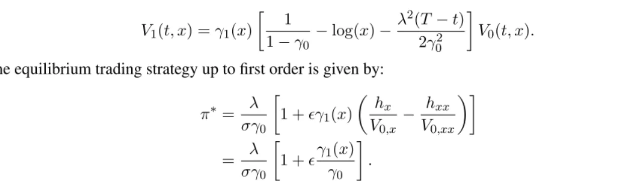
We now compare the Merton optimal strategy, the optimal strategy with first order correction for the slow volatility factor appeared in [15] and our equilibrium strategy with first order correction. Note that the second strategy is equivalent to (36) with only the first fractional term inside the square bracket. We notice that for different levels of the slow factor, the proportions that the two adjustment factors would contribute to the first order correction are different. Figure 2 contains the plots of the three strategies for different ranges of the slow factor. Figures 2a and 2c show that for smallz, the main contributor of the first order correction is the first fractional term inside the square bracket of (71), whereas for larger values ofz, as Figures 2b and 2d suggest, an increasing risk aversion plays the major role instead. The direction to which the first adjustment factor affects the strategy depends on the sign of the correlation factorρ.
2.4 Comparison with Mixture of Power Utility Functions A mixture of power utility functions takes the following form:
Umix(x) =c1 x1−γ1 1−γ1 +c2 x1−γ2 1−γ2 ,
as introduced in Fouque et al.[15], where γ1 6= γ2 and c1, c2 are positive constants. Under this utility
function, the relative risk aversion is not constant any more but decreases inx. Now let us look at a power utility function with wealth-dependent risk aversion:
U(x) = x 1−γ(x)
1−γ(x). (37)
We can choose γ(x) to make Umix(x) = U(x), but in the case of power utility the solution will be a complex-valued function due to the presence ofγ(x)in the exponent ofx. (In contrast, for a mixture of exponential utility functions,γ(x)will be real-valued).
For the case of small wealth-dependence, we have the following expansion:
U(x) = x 1−(γ0+γ1+o(2)) 1−(γ0+γ1+o(2)) =x 1−γ0 −γ1log(x)x1−γ0+o(2) 1−γ0 (1 + γ1 1−γ0 +o(2)) =x 1−γ0 1−γ0 + −x 1−γ0 1−γ0 γ1log(x) + x 1−γ0 1−γ0 γ1 1−γ0 + +o(2)
whereγ1≡γ1(x)can be chosen in such a way that the expansion is also a mixture of power utility functions.
For example, we can setγ1(x)to be:
γ1(x) =
c1xk1+c2xk2
−log(x) +1−1γ 0
0.04 0.06 0.08 0.1 0.12 0.14 0.16 0.18 0.2 0.2 0.4 0.6 0.8 1 1.2 1.4 1.6 z value
proportion of wealth in stock
Merton w/ slow vol corr.
w/ slow vol and risk aversion corr.
(a)ρ=−0.2 0.1 0.2 0.3 0.4 0.5 0.6 0.1 0.2 0.3 0.4 0.5 0.6 0.7 0.8 z value
proportion of wealth in stock
Merton w/ slow vol corr.
w/ slow vol and risk aversion corr.
(b)ρ=−0.2 0.04 0.06 0.08 0.1 0.12 0.14 0.16 0.18 0.2 0.2 0.4 0.6 0.8 1 1.2 1.4 1.6 z value
proportion of wealth in stock
Merton w/ slow vol corr.
w/ slow vol and risk aversion corr.
(c)ρ= 0.2 0.1 0.2 0.3 0.4 0.5 0.6 0.1 0.2 0.3 0.4 0.5 0.6 0.7 0.8 z value
proportion of wealth in stock
Merton w/ slow vol corr.
w/ slow vol and risk aversion corr.
(d)ρ= 0.2
Figure 2: Plots of the equilibrium strategies, in terms of the proportion of total wealth, against the slow stochastic volatility parameterz, in the case of power utility function. We chose the stochastic volatility model to be slow scale CIR(Heston), withµ= 0.15,r= 0,σ(z) =√z,g(z) =
√ z
2 ,ρ=±0.2,T = 5,γ0= 2,γ1= tan
−1(z)and the time
scale isδ= 0.1.
then forxbelonging to the region whereγ1(x)is bounded, the expansion above becomes:
x1−γ0 1−γ0 +x 1−γ0 1−γ0 c1xk1+c2xk2 +o(2) =x 1−γ0 1−γ0 +c1 x1−γ0+k1 1−γ0 +c2 x1−γ0+k2 1−γ0 +o(2) =x 1−γ0 1−γ0 +c1 1−γ0+k1 1−γ0 x1−γ0+k1 1−γ0+k1 +c2 1−γ0+k2 1−γ0 x1−γ0+k2 1−γ0+k2 +o(2)
i.e. a mixture of three power utility functions up to order.
Despite the similarity between the two types of utility functions, i.e. the terminal conditions for the two problems, the portfolio optimization under a mixture of power utility functions remains time-consistent as
the risk aversion always depends on the terminal wealth, which is a random variable revealed at timeT. In our problem here, we have madeγ(·) dependent on the instantaneous level of wealth which becomes the source of time inconsistency.
3
Investment/Consumption Problems with Non-exponential Discounting
In the previous section we have looked at the utility maximization for terminal wealth with time-varying risk aversions by using the method of asymptotic expansions. Here we want to study the investment/consumption problem under non-exponential discounting. We adopt the same two-asset diffusion model (1) for this problem thus we have our wealth process being
dXt= [πt(µ−r)Xt+ (rXt−ct)] dt+πtσXtdWt, (38)
where the additional termctdenotes our instantaneous consumption rate andπtis the proportion of wealth
invested in the risky asset. We define the objective function as:
J(t, x, π,c) =Et,x Z T t ϕ(s−t)U(cs)ds+ϕ(T −t)U(XTπ,c) , (39) whereU(·)is some appropriate utility function to be chosen andϕ(·)is the discount function for the utility derived from consumption. We do not requireϕ(·)to be exponential, which is the source of time inconsis-tency for this problem. As usual, the value function is defined as:
V(t, x) = sup
π,c
J(t, x, π,c). (40) Similar to the utility maximization for terminal wealth case, we have the following result as a consequence of Definition2.4:
Proposition 4. The value functionV(t, x)satisfies the following HJB-type equation:
sup π,c∈R×R+ {∂V ∂t + [πx(µ−r) + (rx−c)] ∂V ∂x + π2 2 σ 2x2∂2V ∂x2 +U(c)}= −Et,x[ Z T t ϕ0(s−t)U(c∗s)ds+ϕ0(T−t)U(XTπ,c∗)] (41) where we have terminal and boundary conditions given by
V(T, x) = 0
V(t,0) = 0,
andc∗sdenotes the equilibrium consumption in the future times≥t.
Proof. For this proof we ignore theϕ(T−t)U(XTπ,c∗)term for simplicity. Using the definition of equilib-rium strategies in(4), let us define:
πs= ( πfors∈[t, t+] π∗fors∈(t+, T] and c s= ( cfors∈[t, t+] c∗ fors∈(t+, T].
i.e. our policyu:= (πs, cs)s∈[t, T]is defined such that it is a uniform and arbitrary perturbation fromu∗for the period[t, t+]and the two strategy will coincide aftert+. Therefore we have
J(t+, Xt+,u) =V(t+, Xt+),
which we take the expectation conditional on(t, x)and plug into the following inequality: V(t, x)≥J(t, x,u) =J(t, x,u)−Et,x[J(t+, Xt+,u)] +Et,x[V(t+, Xt+)] =Et,x Z T t ϕ(s−t)U(cs)ds− Z T t+ ϕ(s−t−)U(c∗s)ds +Et,x[V(t+, Xt+)] ≈Et,x U(ct+)− Z T t+ ϕ0(s−t−)U(cs)ds +Et,x[V(t+, Xt+)],
which in turn is a result of the following simple Taylor expansion for pointtaround(t+):
Z T t ϕ(s−t)U(cs)ds≈ Z T t+ ϕ(s−t−)U(cs)ds+(−) −U(ct+)− Z T t+ ϕ0(s−t−)U(cs)ds) +o(2). Dividing the inequality byand taking the limit→0, we obtain:
Gπ,cV(t, x) +U(ct) +Et,x Z T t ϕ0(s−t)U(c∗s)ds ≤0,
where Gπ,c denotes the infinitesimal generator for V(t, x). If we take the supremum over π andc, the
inequality above becomes equality and we recover the HJB-type equation for V(t, x) less the E[ϕ0(T −
t)U(XTπ,c∗)]term, which can be obtained using the same argument as above. The boundary conditions are straightforward.
Remark 3.1. A first look may suggest that the result(41)above contradicts the remark made in Section 2.1.3
regarding the two-equation characteristics for time inconsistency, since this time we only have one HJB-type equation. In fact, the two-equation feature is masked in the termEt,x[
RT
t ϕ
0(s−t)U(c∗
s)ds], which
char-acterizes the difference on how one’s current self and his immediate future self would value consumption. This is equivalent to saying that the derivative characterizes the difference between the current value func-tion and the continuafunc-tion value funcfunc-tion. If we take the discounting funcfunc-tion to be of exponential type, then the termEt,x[
RT
t ϕ
0(s−t)U(c∗
s)ds]will simply reduce to−rV(t, x), whereris the exponential discounting
rate; and the HJB-type equation will reduce to the classical HJB equation for an investment/consumption problem. However, for all non-exponential-type discounting functions,Et,x[
RT
t ϕ
0(s−t)U(c∗
s)ds]makes
the equation non-local and thus hard to solve. See Ekelandet al.[13] for a numerical treatment of a similar problem using backward integration.
3.1 Approximating a Hyperbolic Discount Function
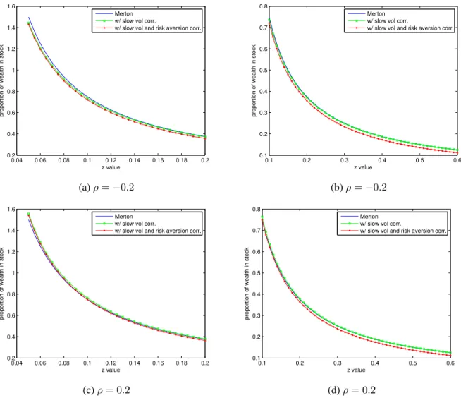
On one hand, the exponential discounting produces explicit solutions but is less realistic. On the other hand, a hyperbolic discount function is in accordance with how people behave but becomes less tractable. There is a clear trade-off between tractability and realisticity. Consider the following discount function:
forα ∈ [0,1]. Whenα = 0, this is an exponential discount function with discount rateδ0. Whenα = 1,
this is a hyperbolic discount function with rateδ1. Forα ∈ (0,1), the discount function will have partial
amount of the features that a hyperbolic discount function has. Now we consider the case whereα= >0is very small, then
ϕ(τ)≈e−δ0τ 1 +∆(τ) +o(2), (43)
where∆(τ) = δ0τ −log(1 +δ1τ)(we can choose other forms of∆(τ)as well). This discount function
will allow us to solve the HJB-type equation(41)using asymptotic expansions in the following subsection. Figure 3 illustrates that this discount function is close to the exponential discounting case for smallwhile it bends towards the hyperbolic discount function. Thus it mimics the hyperbolic discounting feature by a small amount controlled by.
0 1 2 3 4 5 0.4 0.5 0.6 0.7 0.8 0.9 1 t discount rate exponential disc hyperbolic ε=0.05 ε=0.1 ε=0.2 ε=0.3
Figure 3:A comparison of discount functionsexp(−δ0τ),1/(1 +δ1τ)and the one defined by(43)withδ0=δ1= 0.15for various values of.
3.2 Solving the HJB-type Equation Using Asymptotic Expansions
Let us go back to the HJB type equation(41). Using the first order conditions, the maximizations overπ andccan be done separately:
π∗=−µ−r xσ2
Vx
Vxx
and c∗= (U0)−1(Vx), (44)
whereVxdenotes the first derivative w.r.txand so on. We can see thatc∗ is the Legendre transform of the
utility function atVx. From now on we will adopt a power utility function with risk aversionγ:
U(c) = c 1−γ
thus we havec∗= (Vx)−1/γ. We plugπ∗andc∗into(41)to obtain the following nonlinear non-local PDE: Vt− λ2 2 Vx2 Vxx + γ 1−γ(Vx) γ−1 γ +rxV x=−Et,x Z T t ϕ0(s−t)U(c∗s)ds+ϕ0(T−t)U(XTπ,c∗) , (45) with boundary conditionsV(T, x) = 0andV(t,0) = 0.
As a consequence of the expansion(43)for the discount function, we seek a similar expansion for the value function:
V(t, x) =V0(t, x) +V1(t, x) +o(2), (46) which we plug into(45). After grouping terms of different orders, we have the following PDEs for the first two orders: V0,t− λ2 2 V02,x V0,xx + γ 1−γ(V0,x) γ−1 γ +rxV 0,x−δ0V0 = 0, V1,t− λ2 V0,x V0,xx + (V0,x)− 1 γ −rx V1,x+ λ2 2 V2 0,x V02,xxV1,xx−δ0V1 = (47) −Et,x Z T t ∆0(s−t) e−δ0(s−t)[c ∗ 0,s(X (0) s )]1−γ 1−γ ds+ ∆ 0 (T −t)(X (0) T )1−γ 1−γ # ,
where Xs(0) denotes the wealth process under the zeroth order equilibrium investment and consumption
strategiesπ0∗andc∗0. The detail of the decomposition of(45)into(47)can be found in the Appendix.
Note The first equation in (47) can be solved in a fairly standard way with the appropriate boundary con-ditions. Once this is solved, we obtain the zeroth order value function as well as the zeroth order strategies that will give explicit forms for the parameters of the second equation. As we will see later, the solution to the second PDE can be found explicitly. We have therefore managed to bypass the “nonlocal” issue in the HJB-type PDE by using asymptotic expansions. This allows us to avoid the usual numerical procedures as seen for example, in [13].
3.2.1 Zeroth Order Solution
The solution to the zeroth order equation with zero terminal & boundary conditions is very well-known. Using separation of variables method, we seek solutionV0(t, x)of the following form:
V0(t, x) = x 1−γ
1−γ[f(t)]
γ
. (48)
The original PDE problem reduces to the following ODE problem
f0(t) +1−γ γ λ2 2γ +r f(t) +e δ0 γt= 0, (49)
withf(T) = 1. Thus we have
f(t) = −e
A2t+A
3eA2T+A1(T−t)
A1+A2
where A1 = 1−γγ λ2 2γ+r , A2 = δγ0 and A3 = A1+A2+e A2T
eA2T . We can also compute the zeroth order equilibrium strategies: π0∗ = λ σγ andc ∗ 0= x f(t). (51)
3.2.2 First Order Solution
Using the preceding result, we can simplify the first order PDE from(47)into:
V1,t+ λ2 γ +r−1 xV1,x+ λ2 2γ2x 2V 1,xx−δ0V1= (52) Et,x " Z T t ∆0(s−t)e−δ0(s−t)[c ∗ 0,s(X (0) s )]1−γ 1−γ ds+ ∆ 0 (T−t)(X (0) T )1 −γ 1−γ # . In order to deal with the expectation term on the right side, we need the dynamics of the zeroth order wealth processXt(0)under zeroth order equilibrium strategies:
dXt(0)= π∗0(µ−r) +r−f(t)−1Xt(0)dt+π0∗σXt(0)dWt, (53)
which we notice is a lognormal process and we can write out the expectation term explicitly. It follows that E0,x " (Xt(0))1−γ 1−γ # = x 1−γ 1−γe (1−γ)[π∗0(µ−r)+r−f(t)−1− γ 2π ∗2 0 σ2]t. (54) Therefore,(52)becomes V1,t+ λ2 γ +r−1 xV1,x+ λ2 2γ2x 2V 1,xx=δ0V1+ x1−γ 1−γF(t), (55)
whereF(t)denotes the integral: F(t) := Z T t ∆0(s−t)e−δ0(s−t)e(1−γ)[π0∗(µ−r)+r−f(s)−1− γ 2π ∗2 0 σ2]sds.
The ansatzV1(t, x) = x11−−γγg(t)reduces(55)to a first order ODE problem: g0(t) + λ2 2γ +r−1 (1−γ)−δ0 g(t) =F(t), (56) with terminal conditiong(T) = 0, which has a solution given by:
g(t) = Z T t F(s)eB1(s−t)ds, (57) whereB1 := λ2 2γ +r−1 (1−γ)−δ0.
3.2.3 First Order Corrections for Equilibrium Strategies
Proposition 5. We have the following respective first order corrections (to multiply by) to the equilibrium
strategies: π∗1 = 0and c∗1 =−1 γ g(t) f(t)c ∗ 0. (58) Proof. We have V0(t, x) =U(x)f(t)and V1(t, x) =U(x)g(t)
where U(x) is the power utility function with risk aversion γ. For the equilibrium proportion of wealth invested in the risky asset, we have
π∗ ≈ −µ−r xσ2 V0,x+V1,x V0,xx+V1,xx =−µ−r xσ2 U0(x) U00(x) (f(t) +g(t)) (f(t) +g(t)) = µ−r γσ2 ≡π ∗ 0,
whereas for the equilibrium consumption rate, we have
c∗≈(V0,x+V1,x)− 1 γ = (V 0,x)− 1 γ 1− γ V1,x V0,x +o(2) =c∗0 1− γ g(t) f(t) .
We have found that adding a small amount of hyperbolic-discounting feature to the discount function does not change the proportion of wealth invested in the risky asset, while it will affect the consumption rate by a fraction depending on the ratio gf((tt)). Figure 4 illustrates how the approximated equilibrium strategies change over time compared to the optimal one in the exponential discounting case. In general, we find that hyperbolic discounting would encourage one to consume at a faster rate. The fact thatg(t)is negative also means that the value function is more negative compared to the exponential discounting case, indicating a loss of welfare. For relatively larger values of, the equilibrium strategy is clearly non-monotonic. More precisely, the ideal consumption speed starts at some higher level compared to the exponential discounting case and it has a decreasing trend at the beginning. But eventually the consumption speed will start to increase monotonically once we are sufficiently far away from the commencing pointt = 0. In fact, this non-monotonicity feature agrees with the consumption pattern observed in real-life household data, which is one of the main reasons economists support the use of hyperbolic discounting. We also note that similar results were obtained in [13] in which the authors made use of backward numerical integration techniques to solve the full extended HJB equation analogous to (41).
3.3 A Bound for the Value Function: Infinite Horizon Case
In this section we want to illustrate some characteristics of the hyperbolic discounting problem using Laplace transform. Suppose we have an infinite horizon investment/consumption problem instead:
V(x) = sup c E " Z ∞ 0 1 1 +δt c1t−γ 1−γdt # . (59)
The following equation holds for the hyperbolic discount function by Laplace transform:
1 1 +δt = Z ∞ 0 e−τ(t+1δ) δ dτ.
0 1 2 3 4 5 −12 −10 −8 −6 −4 −2 0 t g/f
(a) The ratiofg((tt)).
0 1 2 3 4 5 0.1 0.2 0.3 0.4 0.5 0.6 0.7 0.8 0.9 1 t consumption rate c exponential ε=0.025 ε=0.05 ε=0.075 ε=0.1 (b) Consumption rates.
Figure 4:µ= 0.15,r= 0.05,σ= 0.25,γ= 2,δ0 =δ1 = 0.15andT = 5. We have included the utility of wealth
at timeThere to fix the unbounded consumption rate nearT.
Therefore we have V(x) = sup c Z ∞ 0 E " Z ∞ 0 e−τ t c 1−γ t 1−γdt # e−τδ δ dτ = sup c Z ∞ 0 ¯ J(x, c, τ)e −τ δ δ dτ ≤ Z ∞ 0 sup c ¯ J(x,c, τ)e −τδ δ dτ =βC(x) Z ∞ 0 e−βτ (τ+α)γdτ, (60)
whereC(x) := γγ1x−1γ−γ,α:=−δ(1−γ)−λ2(12γ−γ),β = 1δ andJ¯(x, c, τ)denotes the objective function for the infinite horizon investment problem under consumptioncand exponential discount rateτ, in which case the value function has an explicit solution.
The second line of (60) best illustrates how time inconsistency arises from hyperbolic discounting. Loosely speaking, the integral can be seen as the weighted average of a continuum of optimization problems parameterized by the (exponential-type) discount rateτ. If there is a policy c∗ that can maximize all the objective functions, then the inequality becomes an equality and we can sayc∗is the optimal-for-all policy. Unfortunately, the optimal-for-all policy does not exist most of the time. Nevertheless we can still find a policyc∗∗ that maximizes the integral, i.e. a linearization of the objectives. And it turns out this partic-ular policy c∗∗ is a Pareto optimum that corresponds to a point on the Pareto front of the multi-objective optimization problem. Consequently, the difference between two sides of the inequality corresponds to the distance between a strict optimal value and the Pareto-optimal value under the particular linearization given.
The integral in the last line of(60)can be solved for positive-integer-valuedγ =n∈Z+
Z ∞ 0 e−βτ (τ +α)γdτ =−n! n X j=0 αj j!.
Thus we have produced a bound for the value function in caseγis a positive integer V(x)≤ −βn! n X j=0 αj j!C(x). (61)
3.4 Extension with Proportional Transaction Costs
We extend our study to the situation where proportional transaction cost exists. The dynamics of the portfolio can be represented as below:
dXt(b) = (rXt(b)−ˆct)dt−(1 +κ)dLˆt+ (1−λ)dMˆt
dXt(s) =µXt(s)dt+σXt(s)dWt+dLˆt−dMˆt, (62)
whereXt(b)andXt(s)represent the wealth in the risk-free bank account and in the risky asset (stock) respec-tively. Againˆctis the rate of consumption anddLˆt := ˆltdtanddMˆt:= ˆmtdtdenote the purchase and sell
of the risky asset which will incur proportional transaction costsκandλrespectively.
Our objective function has now been modified into maximizing consumption utility over an infinite horizon because we want to make the analysis simpler. The objective function is given by
J(x(b), x(s),c,ˆ ˆl,mˆ) =E Z ∞ 0 ϕ(s)U(cs)ds X0(b)=x(b), X (s) 0 =x(s) , (63) given the current level of wealthx(b) in the bank account andx(s) in the stock as well as the admissible controlsˆc,m,ˆ ˆl, where the utility functionU(.)is still chosen to be the power type. Now define the value function:
V(x(b), x(s)) = sup ˆ
c,m,ˆ ˆl
J(x(b), x(s),ˆc,ˆl,mˆ). (64) Almost identical to the result from Proposition4, the value function satisfies the HJB-type equation:
sup ˆ c,m,ˆ ˆl (rx(b)−ˆc)Vx(b) +µx(s)Vx(1)+ 1 2σ 2(x(s))2V x(s)x(s)+ [(1−λ)Vx(b)−Vx(s))] ˆm + [Vx(1)−(1 +κ)Vx(b)]ˆl+U(ˆc) =−Ex(b)x(s) Z ∞ 0 ϕ0(s)U(ˆc∗s)ds , (65) only this time there is no time derivative. Whenϕ(·)is exponential type, this becomes the HJB equation that was probably first derived by Davis and Norman [10], who noticed that the desirable strategies for purchase and sell were “bang-bang” type which only took place on the boundaries of the no-transaction region at maximum possible rates.
The homothetic property holds for the value function since we have chosen a power utility function, meaning that
V(ρx(b), ρx(s)) =ρ1−γV(x(b), x(s)), (66) for any positive constantρ. Thus we can write the value functionV(x(b), x(s))into
As a consequence, it is sufficient to study the transformed value functionΦ(z)where we usezto denote the ratiox(b)/x(s).
The problem reduces to a free boundary ODE problem:
(µ−1 2σ 2γ)(1−γ)Φ(z) + (r−µ+σ2γ)zΦ0(z) +1 2σ 2z2Φ00(z) + γ 1−γ Φ0(z)−(1−γ)/γ+Ez " Z ∞ 0 ϕ0(s)[Φ 0(Z s)]−(1−γ)/γ 1−γ ds # = 0, (68)
with free boundary conditions:
Φ0(l)(1−λ+l)−(1−γ)Φ(l) = 0
Φ0(u)(1 +κ+u)−(1−γ)Φ(u) = 0, (69)
where the upper and lower boundaries u andl are to be determined. The ODE (68) is difficult to solve because it involves a free boundary as well as a non-local termEz
h R∞ 0 ϕ 0(s)[Φ0(Zs)]−(1−γ)/γ 1−γ ds i that is the source of time inconsistency. Again let us deal with it using the asymptotic approximation method. We assume the same expansion for the discount functionϕ(·)as in (43). And we seek an expansion for the solutionΦ(z)of the following form:
Φ(z) = Φ0(z) +Φ1(z) +o(2). (70)
At zeroth order, we need to solve the free boundary ODE:
β0Φ0+β1zΦ00 +β2z2Φ000+ γ 1−γ Φ00γ−γ1 = 0 Φ00(l0)(1−λ+l0)−(1−γ)Φ0(l0) = 0 Φ00(u0)(1 +κ+u0)−(1−γ)Φ0(u0) = 0, (71)
withl0, u0to be determined, whereβ0,β1andβ2are constant parameters defined as
β0:= (µ− 1 2σ 2γ)(1−γ)−δ 0, β1 :=r−µ+σ2γ, β2:= 1 2σ 2.
At first order, we need to solve a fixed boundary ODE problem, but with a nonlocal term:
β0Φ1+ β1z+ γ 1−γ(Φ 0 0) −1 γ Φ01+β2z2Φ001+Ez " Z ∞ 0 e−δ0s∆0(s)(Φ 0 0) γ−1 γ 1−γ ds # = 0 Φ01(l0)(1−λ+l0)−(1−γ)Φ1(l0) = 0 Φ01(u0)(1 +κ+u0)−(1−γ)Φ1(u0) = 0, (72)
from which we can compute the first order corrections to the NT boundary as
l1 =− (1−λ+l0)Φ001(l0) +γΦ01(l0) (1−λ+l0)Φ0000(l0) + (1 +γ)Φ000(l0) u1 =− (1 +κ+u0)Φ001(u0) +γΦ01(u0) (1 +κ+u0)Φ0000(u0) + (1 +γ)Φ000(u0), (73)
3.4.1 Zeroth Order Solution
The zeroth order problem (71)is exactly the original problem in [10], which has been shown to have a solution that can be written as
Φ0(z) = 1 1−γ 1−γ γ h1(z) −γ ( z h2(z) )1−γ, (74)
whereh2(z)andh1(z)solve the system below
h02(z) = 1 β2z [R(h2(z))−h1(z)] h01(z) = 1−γ γ h1(z) β2zh2(z) [h1(z)−Q(h2(z))], (75)
with boundary conditions
h2(l0) = l0 l0+ 1−λ , h1(l0) =Q l0 l0+ 1−λ , h2(u0) = u0 u0+ 1 +κ , h1(u0) =Q u0 u0+ 1 +κ , where we defineQ(x) :=− β0 1−γ−β1x+β2γx 2andR(x) :=Q(x) +β
2(1−x)x. This ODE system (75)
can be solved numerically using a shooting method as suggested by [10].
3.4.2 First Order Solution
Recall (72), in order to obtainΦ1(z), we need to solve a fixed boundary ODE, which is numerically
straight-forward except for the source term
Ez " Z ∞ 0 e−δ0s∆0(s)(Φ 0 0(Zs)) γ−1 γ 1−γ ds # ,
which involves a path integral depending on the processZt≡ XYtt. Note that the major issue here is that we do
not have an explicit form forΦ0as it is computed numerically, whereas the nonlocality issue has disappeared similar to the case without transaction cost because of the expansion we have used. To approximate the source term we reply on Monte Carlo method to generate a large number of sample paths forZtup to some
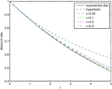
timeT and evaluate the truncated integral for each of these paths using Riemann-sum approximation, after which the estimated expectation can be obtained by taking the average. We first use Ito’s Lemma to get the dynamics for the processZsunder the zeroth order equilibrium strategiesc∗0, dL∗0anddM0∗:
dZt= [(r−µ+
σ2
2 )Zt−c
∗
0,t]dt−σZtdWt−(1 +κ+Zt)dL∗0,t+ (1−λ+Zt)dM0∗,t. (76)
To further simplify the problem we put restrictions on the “Bang-Bang” type strategiesdL∗0anddM0∗so that the processZtdiffuses within the zeroth order NT region but whenever it hits the boundaryl0oru0, it will
be pushed back to the Merton ratio line in the NT region. Figure 5 gives a few sample path of the controlled processXs. We repeat the approximations for a grid of initial valueszand we can smooth out the results
using Fourier-type curve fitting method.
We are left with a second-order ODE with a mixed-type boundary condition to solve. Numerical dis-cretization makes it a linear system of equations Ax = b with A being a tridiagonal matrix. Once we solve this, we can compute the first-order corrections for the NT boundaries as well as for the equilibrium strategies.
0 0.2 0.4 0.6 0.8 1 0.2 0.25 0.3 0.35 0.4 0.45 0.5 0.55 0.6 0.65 t Zt (a)Zs, σ= 0.25 0 0.2 0.4 0.6 0.8 1 1 1.5 2 2.5 t Zt (b)Zs, σ= 0.35
Figure 5: Some realizations ofZswith zeroth order optimal consumption ratec∗0and boundariesl0 andu0.
Note that each time the process hits the boundaries, it will be pushed back to the Merton line inside the NT region.
3.4.3 Numerical Results
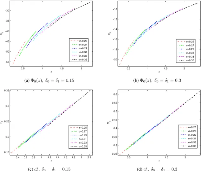
We have numerically solved the zeroth and first order ODE problems using the following set of parameter values: r = 0.05, µ = 0.15, γ = 2, κ = λ = 0.01, δ0 = δ1 = 0.15or0.3 and σ = 0.25 : 0.02 : 0.35. Figure 6 gives illustrations for the zeroth order value functionΦ0(z)and the zeroth order equilibrium
consumption ratec∗0(z). For different volatilityσ, the NT boundaries are different. Figure 7 illustrates the NT region with/without first order corrections. We can see that hyperbolic discounting has the effect of shrinking the NT region, which leads to more frequent trading and rebalancing. This result matches the behavior of typical individual investors who tend to be myopic and impatient and are therefore prone to excessive rebalancing of their investment portfolios. However, whether this is a good or bad thing requires further investigation on this problem.
4
Conclusion
In this article, we have studied several time-inconsistent problems related to portfolio optimization. By using asymptotic methods, we can handle the nonlocality issue that arises from the game-theoretic methodology framework introduced to tackle time-inconsistency. Tractable solutions have been obtained in situations where the time-inconsistent problems can be closely approximated by time-consistent ones, which can also provide a qualitative/directional characterization of the equilibrium investment strategies in more general cases. Our results are intuitive and can describe how differently investors behave in reality and in time consistent settings.