MATHEMATICAL ENGINEERING
TECHNICAL REPORTS
DC Algorithm for
Extended Robust Support Vector Machine
Shuhei FUJIWARA, Akiko TAKEDA and Takafumi
KANAMORI
METR 2014–38 December 2014
DEPARTMENT OF MATHEMATICAL INFORMATICS
GRADUATE SCHOOL OF INFORMATION SCIENCE AND TECHNOLOGY THE UNIVERSITY OF TOKYO
The METR technical reports are published as a means to ensure timely dissemination of scholarly and technical work on a non-commercial basis. Copyright and all rights therein are maintained by the authors or by other copyright holders, notwithstanding that they have offered their works here electronically. It is understood that all persons copying this information will adhere to the terms and constraints invoked by each author’s copyright.
DC Algorithm for
Extended Robust Support Vector Machine
Shuhei Fujiwara∗ Akiko Takeda∗ Takafumi Kanamori†Abstract
Non-convex extensions for Support Vector Machines (SVMs) have been developed for various purposes. For example, robust SVMs attain robustness to outliers using a non-convex loss function, while Extended
ν-SVM (Eν-SVM) extends the range of the hyper-parameter introduc-ing a non-convex constraint. We consider Extended Robust Support Vector Machine (ER-SVM) which is a robust variant of Eν-SVM. ER-SVM combines the two non-convex extensions of robust ER-SVMs and Eν-SVM. Because of two non-convex extensions, the existing algorithm which is proposed by Takeda, Fujiwara and Kanamori needs to be di-vided into two parts depending on whether the hyper-parameter value is in the extended range or not. It also heuristically solves the non-convex problem in the extended range.
In this paper, we propose a new efficient algorithm for ER-SVM. The algorithm deals with two types of non-convex extensions all to-gether never paying more computation cost than that of Eν-SVM and robust SVMs and finds a generalized Karush-Kuhn-Tucker (KKT) point of ER-SVM. Furthermore, we show that ER-SVM includes ex-isting robust SVMs as a special case. Numerical experiments confirm the effectiveness of integrating the two non-convex extensions.
1
Introduction
Support Vector Machine (SVM) is one of the most successful machine learn-ing models, and it has many extensions. The original form of SVM, which is calledC-SVM [6], is popular because of its generalization ability and convex-ity. ν-SVM proposed by [16] is equivalent toC-SVM, and Extendedν-SVM (Eν-SVM) [10] is a non-convex extension of ν-SVM. Eν-SVM introduces a non-convex norm constraint instead of regularization term in the objec-tive function, and the non-convex constraint makes it possible to extend
∗Department of Mathematical Informatics, University of Tokyo, 7-3-1 Hongo,
Bunkyo-ku, Tokyo, 113-8656, Japan. {shuhei fujiwara, takeda}@mist.i.u-tokyo.ac.jp
†Department of Computer Science and Mathematical Informatics, Nagoya University,
the range of the hyper-parameterν. Eν-SVM includes ν-SVM as a special case and Eν-SVM empirically outperforms ν-SVM owing to the extension (see [10]). Furthermore, [21] showed that Eν-SVM minimizes Conditional Value-at-Risk (CVaR) which is a popular convex and coherent risk measure in finance. However, CVaR is sensitive to tail-risks, and the same holds true for Eν-SVM. Unfortunately, it also implies that SVMs might not be sufficiently robust to outliers.
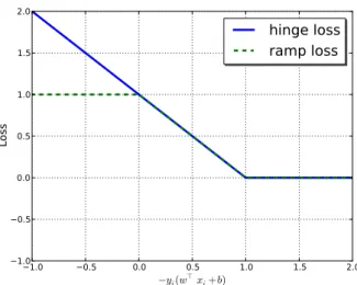
Various non-convex SVMs have been studied with the goal of ensuring robustness to outliers. Indeed, there are many models which are called robust SVM. In this paper, “robust SVMs” means any robust variants of SVMs. Especially, [5, 25] worked on Ramp-Loss SVM which is a popular robust SVM. The idea is to truncate the hinge-loss and bound the value of the loss function by a constant (see Figure 1). Not only hinge-loss, but also any loss functions can be extended by truncating in the same way of ramp-loss. The framework of such truncated loss functions has been studied, for example, in [17, 26]. Xu, Crammer and Schuurmans [25] also proposed Robust Outlier Detection (ROD) which is derived from Ramp-Loss SVM. While Ramp-Loss SVM and ROD are robust variants ofC-SVM, Extended Robust SVM (ER-SVM), recently proposed in [20], is a robust variant of Eν-SVM.
1.1 Non-convex Optimization and DC Programming
The important issue on non-convex extensions is how to solve the difficult non-convex problems. Difference of Convex functions (DC) programming is a powerful framework for dealing with non-convex problems. It is known that various non-convex problems can be formulated as DC programs. For example, every function whose second partial derivatives are continuous ev-erywhere has DC decomposition (cf. [8]).
DC Algorithm (DCA) introduced in [22] is one of the most efficient algorithm for DC programs. The basic idea behind the algorithms is to linearize the concave part and sequentially solve the convex subproblem. The local and global optimality conditions, convergence properties, and the duality of DC programs were well studied using convex analysis [14]. For general DC program, every limit point of the sequence generated by DCA is acritical point which is also calledgeneralized Karush-Kuhn-Tucker (KKT) point. It is remarkable that DCA does not require differentiability in order to assure its convergence properties. Furthermore, it is known that DCA converges quite often to a global solution [9, 11].
In the machine learning literature, a similar method which is called ConCave-Convex Procedure (CCCP) [27] has been studied. The work [18] proposed constrained CCCP to deal with DC constraints, and [19] studied the global convergence properties of (constrained) CCCP, proving that the sequence generated by CCCP converges to a stationary point under
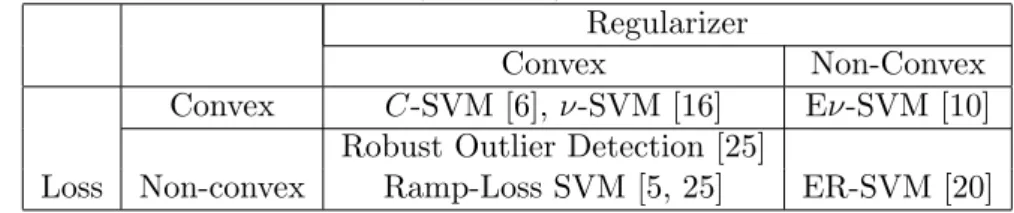
condi-Table 1: Relation of existing models: the models in right (resp. bottom) cell include the models in left (resp. top) cell as a special case.
Regularizer
Convex Non-Convex
Convex C-SVM [6], ν-SVM [16] Eν-SVM [10] Robust Outlier Detection [25]
Loss Non-convex Ramp-Loss SVM [5, 25] ER-SVM [20]
tions such as differentiability and strict convexity. However, since our model is not differentiable, we will use DCA for our problem and take advantage of theoretical results of DCA such as convergence properties.
1.2 Contributions
The main contribution of this paper is a new efficient algorithm based on DCA for ER-SVM. We prove that ER-SVM minimizes the difference of two CVaRs which are known to be convex risk measures. This result allows us to apply DCA to ER-SVM and gives an intuitive interpretation for ER-SVM. The previous algorithm proposed by [20] is heuristics and does not have a theoretical guarantee. However, our new algorithm finds a critical point which is also called generalized KKT point. Though ER-SVM enjoys both of non-convex extensions of Eν-SVM and robust SVMs such as ROD and Ramp-Loss SVM, our new algorithm is simple and comparable to those of Eν-SVM and Ramp-Loss SVM. While the existing algorithm for Eν-SVM [10] needs to use two different procedures depending on the value of the hyper-parameter ν, our new algorithm works with any value of the hyper-parameterν. Besides, our algorithm is similar to Collobert et al.’s algorithm [5] of Ramp-Loss SVM which was shown to be fast.
Furthermore, we clarify the relation of ER-SVM, Ramp-Loss SVM and ROD. We show that ER-SVM includes Ramp-Loss SVM and ROD as a special case in the sense of KKT points. That is, a special case of ER-SVM (whose range of the hyper-parameter ν is limited), Ramp-Loss SVM and ROD share all KKT points. Therefore, as in Table 1, ER-SVM can be regarded not just as a robust variant of Eν-SVM but as a natural extension of Ramp-Loss SVM and ROD.
1.3 Outline of the Paper
This paper is organized as follows: Section 2 is preliminary. In Section 2.1 and 2.2, we introduce existing SVMs and their extensions. Section 2.3 briefly describes definitions and properties of some popular financial risk measures such as CVaR and VaR. Section 3 describes some important
prop-erties of ER-SVM. Section 3.1 gives a DC decomposition of ER-SVM using CVaRs which is a key property for our algorithm. Section 3.2 shows the relation of Ramp-Loss SVM, ROD, and ER-SVM. Section 4 describes our new algorithm after a short introduction of DC programming and DCA. The non-convex extension for regression and its algorithm are briefly discussed in Section 5. Finally, numerical result is presented in Section 6.
2
Preliminary
Here, let us address the binary classification of supervised learning. Suppose we have a set of training samples {(xi, yi)}i∈I where xi ∈ Rn, yi ∈ {−1,1}
and I is the index set of the training samples. I± is the index set such that yi = ±1 and we suppose |I±| >0. SVM learns the decision function
h(x) =⟨w,x⟩+b and predicts the label ofxas ˆy= sign(h(x)). We define
ri(w, b) :=−yi(⟨w,xi⟩+b),
wherein the absolute value of ri(w, b) is proportional to the distance from
the hyperplane ⟨w,x⟩+b= 0 to the samplexi. ri(w, b) becomes negative
if the sample xi is classified correctly and positive otherwise.
Though our algorithm can be extended to nonlinear models using kernel method, we consider linear models for simplicity. Instead, we mention kernel method in Section 3.4.
2.1 Support Vector Machines
2.1.1 Convex SVMs
C-SVM [6] is the most standard form of SVMs, which minimizes the hinge-loss and regularizer:
min w,b 1 2∥w∥ 2+C∑ i∈I [1 +ri(w, b)]+,
where [x]+ := max{0, x} and C > 0 is a hyper-parameter. ν-SVM [16] is formulated as min w,b,ρ 1 2∥w∥ 2−νρ+ 1 |I| ∑ i∈I [ρ+ri(w, b)]+ s.t. ρ≥0, (1)
which is equivalent toC-SVM ifν and C are set appropriately. The hyper-parameterν ∈(0,1] has an upper threshold
ν:= 2 min{|I+|,|I−|}/|I|
and a lower thresholdν. The optimal solution is trivial (w= 0) if ν ≤ν, and the optimal value is unbounded if ν > ν (see [4]). Therefore, we define the range ofν forν-SVM as (ν, ν].
−1.0 −0.5 0.0 0.5 1.0 1.5 2.0 −yi(w⊤xi+b) −1.0 −0.5 0.0 0.5 1.0 1.5 2.0 Lo ss
hinge loss
ramp loss
Figure 1: Loss functions
2.1.2 Non-Convex SVMs
Here, we introduce two types of non-convex extensions for SVMs. The first is Extendedν-SVM (Eν-SVM) [10] which is an extended model of ν-SVM. Eν-SVM introducing a non-convex constraint is formulated as
min ρ,w,b −νρ+ 1 |I| ∑ i∈I [ρ+ri(w, b)]+ s.t. ∥w∥2 = 1. (2)
Eν-SVM has the same set of optimal solutions to ν-SVM if ν > ν, and obtains non-trivial solutions (w̸=0) even if ν ≤ν owing to the constraint
∥w∥2 = 1. Therefore, we define the range of ν for Eν-SVM as (0, ν]. Eν -SVM removes the lower threshold ν of ν-SVM and extends the admissible range of the hyper-parameter ν. It was empirically shown that Eν-SVM sometimes achieves high accuracy in the extended range ofν. We will men-tion other concrete advantages of Eν-SVM over ν-SVM in Section 3.3.
The second is Ramp-Loss SVM which is a robust variant ofC-SVM. The resulting classifier is robust to outliers at the expense of the convexity of the hinge-loss function. The idea behind ramp-loss is to clip large losses with a hyper-parameters≥0. min w,b 1 2∥w∥ 2+C∑ i∈I min{[1 +ri(w, b)]+, s}. (3)
C∈(0,∞) is also a hyper-parameter. Ramp-loss can be described as a differ-ence of hinge-loss functions: therefore ConCave-Convex Procedure (CCCP),
Table 2: If ν is greater than lower threshold (Case C), the non-convex constraint of Eν-SVM and ER-SVM can be relaxed to a convex constraint without changing their optimal solutions. Case C of Eν-SVM is equivalent toν-SVM.
Case N Case C
Range of ν ν≤ν ν < ν≤ν ν < ν
ν-SVM Opt. Val. 0 negative unbounded
Opt. Sol. w=0 admissible –
Range of ν ν≤ν ν < ν≤ν ν < ν
Opt. Val. non-negative negative unbounded Eν-SVM Opt. Sol. admissible admissible –
Constraint ∥w∥2 = 1 ∥w∥2≤1
Range of ν ν≤νµ νµ< ν ≤νµ νµ< ν
Opt. Val. non-negative negative unbounded
ER-SVM Opt. Sol. admissible admissible –
Constraint ∥w∥2 = 1 ∥w∥2≤1
which is an effective algorithm for DC programming, can be applied to the problem (see [5] for details). On the other hand, [25] gave another represen-tation of Ramp-Loss SVM usingη-hinge-loss:
min w,b,η 1 2∥w∥ 2+C∑ i∈I {ηi[1 +ri(w, b)]++s(1−ηi)} s.t. 0≤ηi ≤1, (4)
and applied semidefinite programming relaxation to (4). They also proposed Robust Outlier Detection (ROD):
min w,b,η 1 2∥w∥ 2+C∑ i∈I ηi[1 +ri(w, b)]+ s.t. 0≤ηi≤1, ∑ i∈I (1−ηi) =µ|I|, (5)
which is derived from Ramp-Loss SVM (4). C ∈ (0,∞) and µ ∈[0,1) are hyper-parameters. In the original formulation [25], ROD is defined with an inequality constraint∑i∈I(1−ηi)≤µ|I|but it is replaced by the equality
2.2 Extended Robust Support Vector Machine
Recently, [20] proposed Extended Robust SVM (ER-SVM): min w,b,ρ,η −ρ+ 1 (ν−µ)|I| ∑ i∈I ηi[ρ+ri(w, b)]+ s.t. 0≤ηi ≤1, ∑ i∈I (1−ηi) =µ|I|,∥w∥2 = 1, (6)
whereν ∈(µ,1] andµ∈[0,1) are hyper-parameters.
Note that we relax the 0-1 integer constraintsηi ∈ {0,1} of the original
formulation in [20] and replace∑i∈I(1−ηi)≤µ|I|of the original one by the
equality variant. The relaxation does not change the problem if µ|I| ∈ N. More precisely, ifµ|I| ∈N, ER-SVM (6) has an optimal solution such that
η∗ ∈ {0,1}|I|. In this case, ER-SVM (6) removes µ|I| samples and applies Eν-SVM (2) using the rest, as intended in [20]. Hence, in this paper, we use the formulation (6) and call it ER-SVM.
It can be easily seen that for fixed µ, the optimal value of (6) is de-creasing with respect to ν. Moreover, it is shown in [20, Lemma 1] that the non-convex constraint ∥w∥2 = 1 can be relaxed to ∥w∥2 ≤ 1 without changing the optimal solution as long as the optimal value is negative; just like Eν-SVM, ER-SVM (6) has a threshold (we denote it by νµ) of the hyper-parameterν where the optimal value equals zero and the non-convex constraint∥w∥2 = 1 is essential for ER-SVM withν ≤νµ. The non-convex constraint∥w∥2 = 1 removes the lower threshold of ν and extends the ad-missible range of ν in the same way of Eν-SVM (see Table 2.2). We will show in Section 3.2 that a special case (case C in Table 2.2) of ER-SVM is equivalent to ROD (5) and Ramp-Loss SVM (4) in the way where a special case (case C) of Eν-SVM is equivalent to ν-SVM. Hence, ER-SVM can be seen as a natural extension of Robust SVMs such as ROD and Ramp-Loss SVM. ER-SVM (6) also has an upper thresholdνµwhich makes the problem
bounded similar to Eν-SVM andν-SVM.
2.3 Financial Risk Measures
We define financial risk measures as in [15]. Let us consider the distribution ofri(w, b) :
Ψ(w, b, ζ) :=P(ri(w, b)≤ζ)
= 1
|I||{i∈I :ri(w, b)≤ζ}|.
Forν∈(0,1], letζ1−ν(w, b) be the 100(1−ν)-percentile of the distribution,
known as the Value-at-Risk (VaR) in finance. More precisely, (1−ν)-VaR is defined as
(a) (b)
Figure 2: Difference between VaR and VaR+: VaR+ corresponds to VaR if equation Ψ(w, b, ζ) = 1−ν has no solution (Figure 2(a)).
and (1−ν)-VaR+ which we call (1−ν)-upper-VaR is defined as
ζ1+−ν(w, b) := inf{ζ : Ψ(w, b, ζ)>1−ν}.
The difference between VaR and VaR+ is illustrated in Figure 2.
Conditional Value-at-Risk (CVaR) is also a popular risk measure in fi-nance because of its coherency and computational properties. Formally, (1−ν)-CVaR is defined as
φ1−ν(w, b) := mean of the (1−ν)-tail distribution of ri(w, b),
where the (1−ν)-tail distribution is defined by
Ψ1−ν(w, b, ζ) := 0 forζ < ζ1−ν(w, b) Ψ(w, b, ζ)−(1−ν) ν forζ ≥ζ1−ν(w, b).
The computational advantage of CVaR over VaR is shown by the following theorem.
Theorem 1 (Rockafellar and Uryasev [15]). One has
φ1−ν(w, b) = min ζ F1−ν(w, b, ζ), (7) where F1−ν(w, b, ζ) :=ζ+ 1 ν|I| ∑ i∈I [ri(w, b)−ζ]+.
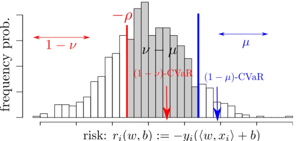
Figure 3: Distribution ofri(w, b): ER-SVM minimizes the mean ofri,i∈I,
in the gray area.
Moreover
ζ1−ν(w, b) =lower endpoint of argmin ζ
F1−ν(w, b, ζ)
ζ1+−ν(w, b) =upper endpoint of argmin
ζ
F1−ν(w, b, ζ)
hold.
Using the property that CVaR is a polyhedral convex function (i.e., piecewise linear and convex function), CVaR can be described as a maximum of linear functions as follows:
φ1−µ(w, b) = max η { 1 µ|I| ∑ i∈I (1−ηi)ri(w, b) : 0≤ηi ≤1, ∑ i∈I (1−ηi) =µ|I| } . (8) We will use the above different representations of CVaR (7) and (8) in the proof of Proposition 1.
3
Properties of Extended Robust SVM
3.1 Decomposition using Conditional Value-at-Risks
Here, we will give an intuitive interpretation to ER-SVM (6) using two CVaRs. Eν-SVM has been shown to minimize (1−ν)-CVaR φ1−ν(w, b) in
[21]. On the other hand, ER-SVM (6) ignores the fractionµ of the samples and solves Eν-SVM using the rest: that is, ER-SVM (6) minimizes CVaR using the rest of the samples. Hence, ER-SVM can be regarded as the one
that minimizes the mean of the distribution of the gray area in Figure 3. The mean of the gray area in Figure 3 can be described using two CVaRs as in [24]:
Proposition 1. ER-SVM (6) is described as a problem minimizing the dif-ference of two convex functions using the two CVaRs:
min w,b 1 ν−µ{νφ1−ν(w, b)−µφ1−µ(w, b)} s.t. ∥w∥2 = 1. (9)
The proof of Proposition 1 is shown in Appendix A.
Since CVaR is convex, this decomposition allows us to apply the existing techniques for DC program to ER-SVM. A similar model which relaxes the non-convex constraint ∥w∥2 = 1 of (9) by ∥w∥2 ≤1 was recently proposed in [23]. As in Table 2.2, Tsyurmasto, Uryasev and Gotoh’s model [23] is a special case (Case C) of ER-SVM, and their model is essentially equivalent to Ramp-Loss SVM and ROD.
3.2 Relationship with Existing Models
Here, we discuss the relation of ER-SVM, ROD, and Ramp-Loss SVM using the KKT conditions shown in Appendix B. Let us begin with showing the equivalence of Ramp-Loss SVM and ROD. Though the formulation of ROD is derived from Ramp-Loss, their equivalence is not particularly discussed in the original paper [25].
Lemma 1(Relation between ROD and Ramp-Loss SVM). Ramp-Loss SVM (4) and ROD (5)share all KKT points in the following sense.
1. Let (w∗, b∗,η∗) be a KKT point of Ramp-Loss SVM (4). Then it is also a KKT point of ROD (5) withµ= |1I|∑i∈I(1−η∗i).
2. A KKT point of ROD(5)having the Lagrange multiplierτ∗for∑i∈I(1−
ηi) =µ|I|is also a KKT point of Ramp-Loss SVM (4) withs= τ
∗
C.
The proof of Lemma 1 is shown in Appendix B.1.
Theorem 2 shows the equivalence of ROD and the special case (Case C in Table 2.2) of ER-SVM.
Theorem 2(Relation between ER-SVM and ROD). Case C of ER-SVM (in Table 2.2), that is (26), and ROD (5)share all KKT points in the following sense.
1. Let(w∗, b∗)satisfy the KKT conditions of ROD (5)and supposew∗ ̸=
0. ∥w1∗∥(w∗, b∗) satisfies the KKT conditions of Case C of ER-SVM
2. Let (w∗, b∗, ρ∗) satisfy the KKT conditions of Case C of ER-SVM. Supposeρ∗ ̸= 0and the objective value is non-zero. ρ1∗(w∗, b∗)satisfies
the KKT conditions of ROD with a corresponding hyper-parameter value.
See Appendix B.2 for the proof of Theorem 2.
From Lemma 1 and Theorem 2, Ramp-Loss SVM and ROD are regarded as a special case (Case C in Table 2.2) of ER-SVM. As we showed in Section 3.1, Tsyurmasto, Uryasev and Gotoh’s model [23] is also equivalent to Case C (in Table 2.2) of ER-SVM. Theorem 2 is similar to the relation between
C-SVM and ν-SVM (which is a special case of Eν-SVM). It was shown that the sets of global solutions ofC-SVM and ν-SVM correspond to each other when the hyper-parameters are set properly [4, 16]. We used KKT conditions to show the relation of non-convex models.
3.3 Motivation for Non-Convex Regularizer
The motivation of the non-convex constraint in Eν-SVM is somewhat not intuitive while that of the robust extension for loss function is easy to un-derstand. Here, we show the motivation of the extension.
As Table 2.2 shows, the non-convex constraint removes the lower thresh-old of the hyper-parameter ν. The extension of the admissible range of ν
has some important advantages. Empirically, [10] showed examples where Eν-SVM outperforms ν-SVM owing to the extended range of ν. They also pointed that small ν achieves sparse solutions since ν controls the number of support vectors.
Here, we show the case where the admissible range of ν for ν-SVM is empty. Theorem 3 gives an explicit condition where C-SVM and ν-SVM obtain a trivial classifier for any hyper-parameter value of C and ν. The conditions also apply to robust SVMs after removing all outliers withηi∗ = 0. Rifkin, Pontil and Verri [13] studied the condition where C-SVM ob-tains a trivial solution. We directly connect their statements toν-SVM and strengthen them as in Theorem 3 by adding a geometric interpretation for
ν-SVM in the case where the admissible range ofν is empty forν-SVM.
Theorem 3. Suppose 0 < |I−| ≤ |I+| without loss of generality. Let us
define Reduced Convex Hull (RCH) [7]:
RCH±(ν) = ∑ i∈I± λixi : ∑ i∈I± λi= 1, 0≤λi ≤ 2 ν|I| for all i . (10)
C-SVM and ν-SVM lead to the trivial classifier (w = 0) for any hyper-parameter values C ∈ (0,∞) and ν ∈ (ν, ν] if and only if a training set
{xi, yi}i∈I satisfies ∑
i∈I−
1
|I−|xi ∈RCH+(ν). When |I−|>|I+|, the above
statement is modified by ∑i∈I+ |I1
The proof is shown in Appendix C.
3.4 Kernelization
Learning methods using linear models can be extended to more powerful learning algorithms by using kernel methods. Here, let us briefly introduce the kernel variant of ER-SVM (6). In kernel methods, the input samplexis mapped intoϕ(x) in a high (even infinite) dimensional inner product space
H, and the classifier of the form h(x) =⟨w, ϕ(x)⟩H+bis learned from the training samples, where ⟨a,b⟩H is the inner product ofa and bin H. The kernel functionk(x,x′) is defined as k(x,x′) =⟨ϕ(x), ϕ(x′)⟩H.
We show how the equality constraint ∥w∥2 = 1 in ER-SVM (6) is dealt with in the kernel method. LetSbe the subspace inHspanned byϕ(xi), i∈
I, and S⊥ be the orthogonal subspace of S. Then the weight vector w is decomposed into w= v+v⊥, where v ∈ S and v⊥ ∈ S⊥. The vectorv⊥
does not affect the value of ri(w, b) =−yi(⟨w, ϕ(xi)⟩H+b). The vector v
is expressed as the linear combination of ϕ(xi) such as v =∑i∈Iαiϕ(xi).
If S = H holds, w = v should hold and the constraint ⟨w,w⟩H = 1 is equivalent with∑i,j∈Iαiαjk(xi,xj) = 1. On the other hand, whenS ̸=H,
i.e., the dimension of S⊥ is not zero, one can prove that the constraint
⟨w,w⟩H = 1 is replaced with the convex constraint ∑i,j∈Iαiαjk(xi,xj) ≤
1, where the fact that the gram matrix (k(xi,xj))i,j is non-negative definite
is used. Indeed, since the objective function depends on w through the componentv, the constraint on wcan be replaced with its projection onto the subspaceS. Thus the above convex constraint is obtained unlessS =H. In such case, the kernel variant of ER-SVM is given as
min α,b,ρ,η −ρ+ 1 (ν−µ)|I| ∑ i∈I ηi[ρ+rki(α, b)]+ s.t. 0≤ηi ≤1, ∑ i∈I (1−ηi) =µ|I|, ∑ i,j∈I αiαjk(xi,xj)≤1, (11) where rki(α, b) = −yi( ∑
j∈Ik(xi,xj)αj +b). When S = H holds, the
in-equality constraint of α should be replaced with the equality constraint.
4
Algorithm
Let us begin with a brief introduction of Difference of Convex functions (DC) program and DC Algorithm (DCA). DC program is formulated by using lower semicontinuous proper convex functions u andv as
min
z {f(z) :=u(z)−v(z) :z∈R
DC Algorithm (DCA) is an efficient algorithm for (12) and theoretically well-studied in e.g., [11]. We shall use simplified DCA, which is the standard form of DCA. Simplified DCA sequentially linearizes the concave part in (12) and solves convex subproblems as follows:
zk+1 ∈argmin
z {
u(z)−(v(zk) +⟨z−zk,gk⟩)}, (13)
wheregk∈∂v(zk) is a subgradient ofvatzk. The sequence{zk}generated
by Simplified DCA has the following good convergence properties:
• the objective value is decreasing (i.e., f(zk+1)≤f(zk)),
• DCA has linear convergence,
• every limit point of the sequence{zk}is acritical point ofu−v, which
is also calledgeneralized KKT point.
z∗ is said to be a critical point of u−v if ∂u(z∗)∩∂v(z∗) ̸=∅. It implies that a critical point z∗ has gu ∈ ∂u(z∗) and gv ∈ ∂v(z∗) such that gu− gv = 0 which is a necessary condition for local minima. When (12) has a convex constraintz ∈Z, we can define the critical point by replacinguwith
u(z) +δ(z |Z), where δ(z|Z) is an indicator function equal to 0 if z ∈Z
and +∞ otherwise.
4.1 DCA for Extended Robust SVM
As shown in Section 3.1, ER-SVM (6) can be described as a difference of CVaRs (9). Moreover, (9) can be reformulated into a problem of minimizing the DC objective upon a convex constraint using a sufficiently large constant
t:
min
w,b νφ1−ν(w, b)−µφ1−µ(w, b)−t∥w∥
2
s.t. ∥w∥2 ≤1. (14)
This reformulation is a special case of the exact penalty approach (see [11, 12]). There exists to such that (9) and (14) have the same set of optimal
solutions for all t > to. We can estimate an upper bound of to in our case
by invoking the following lemma.
Lemma 2. If t≥0 in (14) is sufficiently large such that the optimal value of (14) is negative, (9)and (14) have the same set of optimal solutions.
The key point in the proof of Lemma 2 is that CVaR has a positive homogeneity (i.e., φ(aw, ab) = aφ(w, b) for all a such that a ∈ R, a > 0). This is a well-known property of coherent risk measures such as CVaR (e.g., [1]).
Proof of Lemma 2. Let (w∗, b∗) be an optimal solution of (14) and suppose to the contrary that ∥w∗∥ < 1. (∥ww∗∗∥, b
∗
∥w∗∥) achieves a smaller objective
value than (w∗, b∗) since
νφ1−ν( w∗ ∥w∗∥, b∗ ∥w∗∥)−µφ1−µ( w∗ ∥w∗∥, b∗ ∥w∗∥)−t ∥w∗∥2 ∥w∗∥2 = 1 ∥w∗∥{νφ1−ν(w ∗, b∗)−µφ 1−µ(w∗, b∗)−t∥w∗∥} ≤ ∥ 1 w∗∥{νφ1−ν(w ∗, b∗)−µφ 1−µ(w∗, b∗)−t∥w∗∥2} | {z } negative < νφ1−ν(w∗, b∗)−µφ1−µ(w∗, b∗)−t∥w∗∥2.
However, this contradicts the optimality of (w∗, b∗). Therefore, the optimal solution of (14) satisfies ∥w∥ = 1, which implies that it is also optimal to (9).
Therefore, (14) is represented as the following DC program: min w,b{u(w, b)−v(w, b)} (15) where u(w, b) =δ(w|W) +νφ1−ν(w, b) v(w, b) =µφ1−µ(w, b) +t∥w∥2 W ={w| ∥w∥2≤1}.
Here, we apply simplified DCA to the problem (15). At kth iteration of simplified DCA, we solve a subproblem as in (13) linearizing the concave part. Let (wk, bk) be the solution obtained in the previous iterationk−1 of simplified DCA. The subproblem of simplified DCA for (15) is described as
min
w,b νφ1−ν(w, b)−µ⟨g k
w,w⟩ −µgbkb−2t⟨wk,w⟩
s.t. ∥w∥2≤1, (16)
where (gkw, gbk) ∈ ∂φ1−µ(wk, bk). ∂φ1−µ is the subdifferential of φ1−µ and
(gk
w, gkb) is a subgradient of φ1−µ at (wk, bk). The optimal solution of (16)
is denoted by (wk+1, bk+1). We will show how to calculate a subgradient (gkw, gkb) and how to choose a sufficiently large constantt.
Subdifferential of CVaR Here, we show how to calculate the subdif-ferential of CVaR (8). The following technique is described in [24]. The
subdifferential of CVaR at (wk, bk) is ∂wφ1−µ(wk, bk) = co { − 1 µ|I| ∑ i∈I (1−ηik)yixi :ηk∈H(wk, bk) } , ∂bφ1−µ(wk, bk) = co { − 1 µ|I| ∑ i∈I (1−ηik)yi :ηk∈H(wk, bk) } ,
where coX is the convex hull of the setX and
H(wk, bk) = argmax η { ∑ i∈I (1−ηi)ri(wk, bk) : ∑ i∈I (1−ηi) =µ|I|,0≤ηi≤1 } . (17) We can easily find an optimal solutionηk∈H(wk, bk) by assigning 0 toηik
in descending order ofri(wk, bk) for alli.
Efficient Update oft The update of the large constanttin each iteration makes our algorithm more efficient. We propose to use, in thekth iteration,
tk such that
tk> νφ1−ν(wk, bk)−µφ1−µ(wk, bk). (18)
The condition (18) ensures the optimal value of (14) being negative, since the solution (wk, bk) in the previous iteration has achieved a negative objective value. With such tk, Lemma 2 holds.
Explicit Form of Subproblem We are ready to describe the subproblem (16) explicitly. Using the above results and substituting (7) forφ1−ν(w, b),
(16) results in min w,b,ρ,ξ −νρ+ 1 |I| ∑ i∈I ξi− 1 |I| ∑ i∈I (1−ηik)ri(w, b)−2tk⟨wk,w⟩ s.t. ξi ≥ρ+ri(w, b), ξi≥0,∥w∥2≤1. (19)
Hence, we summarize our algorithm as Algorithm 1.
5
Regression
Some parts of our analysis and algorithm can be applied to regression. Re-gression models seek to estimate a linear functionf(x) = ⟨w,x⟩+b based on data (xi, yi)∈Rn×R,i∈I. ν-Support Vector Regression (ν-SVR) [16]
is formulated as min w,b,ϵ 1 2C∥w∥ 2+νϵ+ 1 |I| ∑ i∈I [|⟨w,xi⟩+b−yi| −ϵ]+, (20)
Algorithm 1 DCA for Difference of CVaRs
Input: µ ∈ [0,1), ν ∈ (µ, νµ], (w0, b0) such that ∥w0∥2 = 1 and a small
valueϵ1, ϵ2 >0. 1: k= 0. 2: repeat 3: Selectηk∈H(wk, bk) arbitrarily. 4: Updatetk as tk←max { 0,νφ1−ν(w k, bk)−µφ 1−µ(wk, bk) 1−ϵ2 } . 5: 6: (wk+1, bk+1) = a solution of subproblem (19). 7: k←k+ 1. 8: until f(wk, bk)−f(wk+1, bk+1) < ϵ1 where f(w, b) = νφ1−ν(w, b)− µφ1−µ(w, b).
where C ≥ 0 and ν ∈ [0,1) are hyper-parameters. Following the case of classification, we formulate robustν-SVR as
min w,b,ϵ,η 1 2C∥w∥ 2+ (ν−µ)ϵ+ 1 |I| m ∑ i=1 ηi[|w⊤xi+b−yi| −ϵ]+ s.t. 0≤ηi ≤1, ∑ i∈I (1−ηi) =µ|I|, (21)
whereC ≥0,ν ∈(µ,1] andµ∈[0,1) are hyper-parameters. Let us consider the distribution of
rregi (w, b) :=|⟨w,xi⟩ −yi|.
φreg1−ν(w, b) (resp. φreg1−µ(w, b)) denotes (1−ν)-CVaR (resp. (1−µ)-CVaR) of the distribution. Robustν-SVR (21) can be decomposed by the two CVaRs as min w,b 1 2C∥w∥ 2+νφreg 1−ν(w, b)−µφ reg 1−µ(w, b). (22)
Since (22) is decomposed to the convex part and concave part, we can use simplified DCA for robust ν-SVR.
6
Numerical Results
We compared ER-SVM with ramp-loss SVM by CCCP [5] and Eν-SVM [10]. The hyper-parameter s of the ramp-loss function was fixed to 1, and
6.1 Synthetic Datasets
We used synthetic data generated by following the procedure in [25]. We generated two-dimensional samples with labels +1 and−1 from two normal distributions with different mean vectors and the same covariance matrix. The optimal hyperplane for the noiseless dataset is h(x) = x1 −x2 = 0
with w = √1
2(1,−1) and b = 0. We added outliers only to the training
set with the label −1 by drawing samples uniformly from a half-ring with center 0, inner-radius R = 75 and outer-radius R + 1 in the space x of
h(x) > 0. The training set contains 50 samples from each class (i.e., 100 in total) including outliers. The ratio of outliers in the training set was set to a value from 0 to 5%. The test set has 1000 samples from each class (i.e., 2000 in total). We repeated the experiments 100 times, drawing training and test sets every repetition. We found the best parameter setting from 9 candidates,ν = 0.1,0.2, . . . ,0.9 andC = 10−4,10−3, . . . ,104. Figure 4(a) shows the outlier ratio and the test error of each models. ER-SVM (µ = 0.05) achieved good accuracy especially when the outlier ratio was large.
0 1 2 3 4 5 Outlier Ratio (%) 0.018 0.020 0.022 0.024 0.026 0.028 0.030 Test Er ror
ER-SVM
Ramp-Loss
E
ν-SVM
(a) Synthetic data
0.1 0.2 0.3 0.4 0.5 0.6 0.7 0.8 ν 0.26 0.28 0.30 0.32 0.34 0.36 0.38 0.40 Te st E rr or Test Error ¯νµ
(b) Test error (liver)
0.1 0.2 0.3 0.4 0.5 0.6 0.7 0.8 ν 0.05 0.10 0.15 0.20 0.25 0.30 0.35 0.40 0.45 Tim e ( se c)
Time
¯νµ(c) Comp. time (liver)
−4 −2 0 2 4 −4 −2 0 2 4 ER-SVM (d) Nontrivial classifier 0 10 20 30 40 50 Iteration 10-3 10-2 10-1 100 O bj ct iv e Va lu e t: auto update t =0.1 t =0.5 (e) Convergence 0.0 0.1 0.2 0.3 0.4 0.5 0.6 0.7 ν 0 50 100 150 200 250 300 win draw (f) Objective value
Figure 4: (a) shows the average errors for synthetic dataset. (b) is an example where ER-SVM achieved the minimum test error withν ≤νµin the extended parameter range. (c) shows the computational time of Algorithm 1. (d) shows the example where ER-SVM obtains a non-trivial classifier, though C-SVM, ν-SVM and ramp-loss SVM obtain trivial classifiers w =
0. (e) implies that our update rule of tk as in (18) achieves much faster
convergence. (f) shows how many times ER-SVM achieves smaller objective values than the heuristic algorithm in 300 trials.
T able 3: Av erage error of real datasets in 10 trials Dataset Dim # train # test ( ν ,ν ) Outlier Ratio ER-SVM Ramp E ν -SVM Liv er 6 345 10-cross (0 . 72 , 0 . 84) 0% 0 . 270 N 0 . 284 0 . 290 N ( R = 5) 1% 0 . 284 N 0 . 287 0 . 310 C 3% 0 . 278 N 0 . 417 0 . 490 C Diab etes 8 768 10-cross (0 . 52 , 0 . 70) 0% 0 . 227 N 0 . 219 0 . 224 N ( R = 10) 3% 0 . 219 N 0 . 232 0 . 238 C 5% 0 . 236 N 0 . 289 0 . 288 N Heart 13 270 10-cross (0 . 33 , 0 . 89) 0% 0 . 156 C 0 . 159 0 . 156 C ( R = 50) 3% 0 . 174 C 0 . 170 0 . 185 C 5% 0 . 167 C 0 . 200 0 . 219 C Splice 60 1000 10-cross (0 . 37 , 0 . 97) 0% 0 . 186 N 0 . 199 0 . 188 C ( R = 100) 5% 0 . 188 N 0 . 254 0 . 295 C Adult 123 1605 30956 (0 . 32 , 0 . 49) 0% 0 . 159 N 0 . 159 0 . 158 C ( R = 150) 5% 0 . 157 C 0 . 166 0 . 161 C V ehicle (class 1 vs rest) 18 846 10-cross (0 . 42 , 0 . 50) 0% 0 . 201 N 0 . 204 0 . 201 N ( R = 100) 5% 0 . 217 N 0 . 242 0 . 371 C Satimage (class 6 vs rest) 36 4435 2000 (0 . 21 , 0 . 47) 0% 0 . 102 N 0 . 105 0 . 106 C ( R = 150) 3% 0 . 100 N 0 . 143 0 . 184 C
We used the datasets of the UCI repository [2] and LIBSVM [3]. We scaled all attributes of the original dataset from−1.0 to 1.0. We generated outliers ˆx uniformly from a ring with center 0 and radius R and assigned the wrong label ˆy to ˆx by using the optimal classifiers of Eν-SVM. The radius R of generating outliers was set properly so that the outliers would have an impact on the test errors. The best parameter was chosen from 9 candidates, ν ∈(0, ν] with equal intervals and C = 5−4,5−3, . . . ,54. These parameters are decided using 10-fold cross validation and the error is the average of 10 trials. Table 3 shows the results for real datasets. ER-SVM often achieved smaller test errors than ramp-loss SVM and Eν-SVM, and the prediction performance of ER-SVM were very stable to increasing the outlier ratio. ’N’ in Table 3 implies that ER-SVM (or Eν-SVM) achieved the best accuracy with ν ≤ νµ (or ν ≤ ν) and ’C’ implies that the best accuracy was achieved withνµ< ν (orν < ν).
6.3 Effectiveness of the Extension
Let us show an example where the extension of parameter range works. We used 30% of the liver dataset for training and 70% for the test. We tried the hyper-parameterν from 0.1 to the νµ with the interval 0.01 and µ is fixed
to 0.03. The computational time is the average of 100 trials. Figure 4(b) and (c) show the test error and the computational time. The vertical line is an estimated value ofνµ. The extension for parameter range corresponds to the left side of the vertical line where the non-convex constraint ∥w∥2 = 1 worked. ER-SVM withν < νµ can find classifiers which ROD or ramp-loss SVM can not find. In Figure 4(b), ER-SVM achieved the minimum test error withν≤νµ. In Figure 4(c) it seems that the computational time does not change so much though the non-convex constraint works in the left side of the vertical line. Note that the computational time becomes large around
ν = 0.3. The optimal margin variable ρ is zero around ν = 0.3. It might make the problem difficult and numerically unstable.
Figure 4(d) shows an example of the effectiveness of the non-convex constraint ∥w∥2 = 1. When the number of the samples in each class is imbalanced or the samples in two classes are largely overlapped as in Figure 4(d),C-SVM,ν-SVM, and ramp-loss SVM obtain trivial classifiers (w=0) while ER-SVM obtains a non-trivial classifier. That is, this figure implies the effectiveness of the non-convex constraint ∥w∥2 = 1.
6.4 Efficient Update of tk
We show the effectiveness of the auto update rule of the constant tk as in
(18). We used the liver dataset. Figure 4(e) implies that our auto update rule achieves much faster convergence than the fixed constantt= 0.1 or 0.5.
6.5 Comparison of DCA and Heuristics
We compared the performance of the heuristic algorithm [20] for ER-SVM and our new algorithm based on DCA. We ran the two algorithm on liver-disorder data set and computed the difference of the objective values. Initial values are selected from uniform random distribution on unit sphere and the experiments were repeated 300 times. Since the hyper-parameter µ is automatically selected in the heuristic algorithm, we set correspondingµfor DCA. To compare the quality of the solutions obtained by each algorithm, we counted how many times our algorithm (DCA) achieved smaller objective values than the heuristics. We counted ‘win’, ‘lose’, ‘draw’ cases in 300 trials. However it is difficult to judge whether a small difference in objective values is caused by numerical error or the difference of local solutions. Hence, we call ‘win’ (or ‘lose’) for the case where DCA achieves a smaller (or larger) objective value than the heuristic algorithm by more than 3% difference. Figure 4(f) shows the result. Our algorithm (DCA) tends to achieve ‘win’ or ‘draw’ in many cases. Some papers (e.g., [9, 11]) state that DCA tends to converge to a global solution. This result may support the discussion.
7
Conclusions
We gave theoretical analysis to ER-SVM: we proved that ER-SVM is a natural extension of ROD and discuss the condition under which such the extension works. Furthermore, we proposed a new efficient algorithm which has theoretically good properties. Numerical experiments showed that our algorithm worked efficiently.
We might be able to speed up the proposed algorithm by solving the dual of subproblems (19). The problem has the similar structure with the dual SVM and Sequential Minimal Optimization (SMO) might be applicable to the dual of subproblems.
References
[1] P. Artzner, F. Delbaen, J. Eber, and D. Heath. Coherent measures of risk. Mathematical Finance, 9:203–228, 1999.
[2] C. L. Blake and C. J. Merz. UCI repository of machine learning databases, 1998.
[3] C. C. Chang and C. J. Lin. Libsvm : A library for support vector machines. Technical report, Department of Computer Science, National Taiwan University, 2001.
[4] C.-C. Chang and C.-J. Lin. Training ν-support vector classifiers: The-ory and algorithms. Neural Computation, 13(9):2119–2147, 2001.
[5] R. Collobert, F. Sinz, J. Weston, and L. Bottou. Trading convexity for scalability. In International Conference on Machine Learning, pages 129–136, 2006.
[6] C. Cortes and V. Vapnik. Support-vector networks. Machine Learning, 20:273–297, 1995.
[7] D.J. Crisp and C.J.C. Burges. A geometric interpretation of ν-svm classifiers. In Neural Information Processing Systems 12, pages 244– 250, 2000.
[8] R. Horst and H. Tuy. Global Optimization: Deterministic Approaches. Springer-Verlag, Berlin, 3rd edition, 1996.
[9] H. A. Le Thi and T. Pham Dinh. The dc (difference of convex functions) programming and dca revisited with dc models of real world nonconvex optimization problems. Annals of Operations Research, 133(1-4):23–46, 2005.
[10] F. Perez-Cruz, J. Weston, D. J. L. Hermann, and B. Sch¨olkopf. Ex-tension of theν-SVM range for classification. In Advances in Learning Theory: Methods, Models and Applications 190, pages 179–196, Ams-terdam, 2003. IOS Press.
[11] T. Pham Dinh and H. A. Le Thi. Convex analysis approach to d.c. programming: Theory, algorithms and applications. Acta Mathematica Vietnamica, 22(1):289–355, 1997.
[12] T. Phanm Dinh, H. A. Le Thi, and Le D. Muu. Exact penalty in d.c. programming. Vietnam Journal of Mathematics, 27(2):169–178, 1999. [13] Ryan M. Rifkin, Massimiliano Pontil, and Alessandro Verri. A note on
support vector machine degeneracy. In Algorithmic Learning Theory, pages 252–263, 1999.
[14] R. T. Rockafellar.Convex Analysis. Princeton University Press, Prince-ton, 1970.
[15] R. T. Rockafellar and S. Uryasev. Conditional value-at-risk for general loss distributions. Journal of Banking & Finance, 26(7):1443–1472, 2002.
[16] B. Sch¨olkopf, A. Smola, R. Williamson, and P. Bartlett. New support vector algorithms. Neural Computation, 12(5):1207–1245, 2000. [17] Xiaotong Shen, George C Tseng, Xuegong Zhang, and Wing Hung
Wong. On ψ-learning. Journal of the American Statistical Associa-tion, 98(463):724–734, 2003.
[18] A. J. Smola, S. V. N. Vishwanathan, and T. Hofmann. Kernel meth-ods for missing variables. In In Proceedings of the Tenth International Workshop on Artificial Intelligence and Statistics, pages 325–332, 2005. [19] Bharath K. Sriperumbudur and Gert R. G. Lanckriet. A proof of con-vergence of the concave-convex procedure using zangwill’s theory. Neu-ral Computation, 24(6):1391–1407, 2012.
[20] A. Takeda, S. Fujiwara, and T. Kanamori. Extended robust support vector machine based on financial risk minimization. Neural Computa-tion, 26(11):2541–2569, 2014.
[21] A. Takeda and M. Sugiyama. ν-support vector machine as conditional value-at-risk minimization. In International Conference on Machine Learning, pages 1056–1063, 2008.
[22] Pham Dinh Tao. Duality in dc (difference of convex functions) optimiza-tion. Subgradient methods. In Trends in Mathematical Optimization, pages 277–293. 1988.
[23] P. Tsyurmasto, S. Uryasev, and J. Gotoh. Support vector classification with positive homogeneous risk functionals. Technical report, 2013. [24] D. Wozabal. Value-at-risk optimization using the difference of convex
algorithm. OR Spectrum, 34:861–883, 2012.
[25] L. Xu, K. Crammer, and D. Schuurmans. Robust support vector ma-chine training via convex outlier ablation. In AAAI, pages 536–542. AAAI Press, 2006.
[26] Y. Yu, M. Yang, L. Xu, M. White, and D. Schuurmans. Relaxed clip-ping: A global training method for robust regression and classifica-tion. InNeural Information Processing Systems, pages 2532–2540. MIT Press, 2010.
[27] A. L. Yuille and A. Rangarajan. The concave-convex procedure. Neural Computation, 15(4):915–936, 2003.
A
Proof of Proposition 1
The objective function of ER-SVM (6) under the constraints can be equiv-alently rewritten as ζ+ 1 (ν−µ)|I| ∑ i∈I ηi[ri(w, b)−ζ]+ = 1 ν−µ { (ν−µ)ζ+ 1 |I| ∑ i∈I ηi[ri(w, b)−ζ]+ } = 1 ν−µ { (ν−µ)ζ+ 1 |I| ∑ i∈I [ri(w, b)−ζ]+− 1 |I| ∑ i∈I (1−ηi)[ri(w, b)−ζ]+ } = 1 ν−µ { νζ+ 1 |I| ∑ i∈I [ri(w, b)−ζ]+− 1 |I| ∑ i∈I (1−ηi){[ri(w, b)−ζ]++ζ} } .
The last equality is obtained by using a constraint, ∑i∈I(1−ηi) =µ|I|, of
ER-SVM (6).
Now we show that the term in the last equation 1
|I|
∑ i∈I
(1−ηi){[ri(w, b)−ζ]++ζ}
can be written as |1I|∑i∈I(1−ηi)ri(w, b) by showing thatri(w∗, b∗)−ζ∗≥0
holds for anyi whenever 1−ηi∗ >0 at the optimal solution (w∗, b∗, ζ∗,η∗) of (6). Here we assume thatri(w∗, b∗),∀i, are sorted into descending order;
r1(w∗, b∗)≥r2(w∗, b∗)≥. . .. Then η∗ should be
η1∗=. . .=η⌊∗µ|I|⌋= 0, η⌊∗µ|I|⌋+1>0, η∗⌊µ|I|⌋+2 =. . .1.
Note thatζ∗ must be an optimal solution of the problem:
min ζ ζ+ 1 (ν−µ)|I| |I| ∑ i=⌊µ|I|⌋+1 ηi∗[ri(w∗, b∗)−ζ]+ s.t. ∥w∥2= 1.
The problem is regarded as minimizing (1−α)-CVaR, where α := ν1−−µµ (>0), for the truncated distribution with⌊µ|I|⌋samples removed. Theorem 1 ensures that
r⌊µ|I|⌋+1(w∗, b∗)≥ζ1+−α(w∗, b∗)≥ζ∗,
which implies that ri(w∗, b∗)−ζ∗≥0 holds for the indices havingηi<1.
Therefore, we can rewrite the objective function of ER-SVM (6) by 1 ν−µ { νζ+ 1 |I| ∑ i∈I [ri(w, b)−ζ]+− 1 |I| ∑ i∈I (1−ηi)ri(w, b) } . (23)
By using (7) for the first two terms of (23) and using (8) for the last term, we further rewrite (23) as
1
ν−µ{νφ1−ν(w, b)−µφ1−µ(w, b)},
which is the objective function of (9). This implies that ER-SVM (6) is described as the form of (9).
B
KKT Conditions for ER-SVM, ROD, and
Ramp-Loss SVM
To define the KKT conditions, we show differentiable formulations of Case C of ER-SVM (6), ROD (5), and Ramp-Loss SVM (4).
Continuous Ramp-Loss SVM: min w,b,η,ξ 1 2∥w∥ 2+C∑ i∈I {ηiξi+s(1−ηi)} s.t. 0≤ηi ≤1, ξi ≥1 +ri(w, b), ξi ≥0 (24) Continuous ROD: min w,b,η,ξ 1 2∥w∥ 2+C∑ i∈I ηiξi s.t. 0≤ηi≤1, ∑ i∈I (1−ηi) =µ|I|, ξi≥1 +ri(w, b), ξi ≥0 (25)
Continuous ER-SVM (limited to Case C in Table 2.2):
min w,b,ρ,η,ξ −ρ+ 1 (ν−µ)|I| ∑ i∈I ηiξi s.t. 0≤ηi ≤1, ∑ i∈I (1−ηi) =µ|I| ξi ≥ρ+ri(w, b), ξi≥0,∥w∥2 ≤1 (26)
KKT Conditions of (24) using (w, b,η,ξ;λ,α,β,γ): ∑ i∈I λiyi= 0, (27a) γiξi= 0, (27b) αi(ηi−1) = 0, (27c) βiηi= 0, (27d) λi, αi, βi, γi,≥0, (27e) 0≤ηi≤1, (27f) ξi≥0, (27g) λi{1−ξi+ri(w, b)}= 0, (28a) −ri(w, b)≥1−ξi, (28b) w=∑ i∈I λiyixi, (28c) Cηi−λi−γi= 0, (28d) and Cξi−Cs+αi−βi = 0 (29) KKT Conditions of (25) using (w, b,η,ξ;λ,α,β,γ, τ): (27), (28), Cξi−τ+αi−βi = 0, (30) and ∑ i∈I (1−ηi) =µ|I| (31) KKT Conditions of (26) using (w, b, ρ,η,ξ;λ,α,β,γ, τ, δ):
(27), (31), and λi{ρ−ξi+ri(w, b)}= 0, (32a) −ri(w, b)≥ρ−ξi, (32b) 2δw=∑ i∈I λiyixi, (32c) ηi |I|−λi−γi = 0, (32d) 1 |I|ξi−τ +αi−βi = 0, (32e) ∑ i∈I λi =ν−µ, (32f) δ(∥w∥2−1) = 0, (32g) δ≥0 (32h) B.1 Proof of Lemma 1
The difference between the KKT conditions of Ramp-Loss SVM (24) and ROD (25) is only (29), (30), and (31).
Note that a KKT point (w∗, b∗,η∗) of Ramp-Loss SVM (24) satisfies the KKT conditions of ROD (25) withµ= |1I|∑i∈I(1−ηi∗). On the other hand, a KKT point of (25) whose Lagrange multiplier for ∑i∈I(1−ηi) =µ|I| is
τ∗ satisfies the KKT conditions of Ramp-Loss SVM (24) with s= τC∗.
B.2 Proof of Theorem 2
We will show the first statement. Let (w∗, b∗,η∗,ξ∗) be a KKT point of (25) with hyper-parameter C and Lagrange multipliers (λ∗,α∗,β∗,γ∗, τ∗). Supposew∗ ̸=0. Then (∥ww∗∗∥, b
∗
∥w∗∥,η∗, ξ ∗
∥w∗∥, ρ∗ = ∥w1∗∥) is a KKT point of
(26) with Lagrange multipliersC1|I|(λ∗,∥wα∗∗∥, β ∗ ∥w∗∥,γ∗, τ ∗ ∥w∗∥) andδ= ∥w ∗∥ 2C|I|.
We will show the second statement. Let (w∗, b∗,η∗,ξ∗, ρ∗) be a KKT point of (26) with Lagrange multipliers (λ∗,α∗,β∗,γ∗, τ∗, δ∗). Supposeρ∗ ̸= 0. If δ∗ ̸= 0, (wρ∗∗,b
∗
ρ∗,η∗, ξ∗
ρ∗) satisfies the KKT conditions of (25) with
La-grange multipliers 21δ∗(λ ∗ ρ∗,α∗,β∗, γ∗ ρ∗, τ∗) and hyper-parameter C= 1 δ∗ρ∗|I|.
Now, we will proveδ∗ ̸= 0 using the assumption of non-zero optimal value. Consider the following problem which fixesη of (26) toη∗:
min w,b,ρ,ξ −ρ+ 1 (ν−µ)|I| ∑ i∈I η∗iξi s.t. ∥w∥2≤1,−ri(w, b)≥ρ−ξi, ξi ≥0. (33)
The KKT conditions of (33) are as follows. 2δw=∑ i∈I λiyixi, ∑ i∈I λiyi= 0, ηi |I|−λi−γi = 0, ∑ i∈I λi =ν−µ, λi{ρ−ξi+ri(w, b)}, γiξi= 0, δ(∥w∥2−1) = 0, δ, λi, γi,≥0, −ri(w, b)≥ρ−ξi, ξi ≥0.
(w∗, b∗,ξ∗, ρ∗) is also a KKT point of (33) with the same Lagrange multipli-ers (λ∗,γ∗, δ∗) as (26). Moreover, (w∗, b∗,ξ∗, ρ∗) is not only a KKT point but also an optimal solution of (33) because (33) is a convex problem. Since the objective function of the dual problem of (33) is−δ(∥w∥2+ 1),δ∗ = 0 if and only if the objective value is zero. Then, we can see that δ∗̸= 0 under the assumption of non-zero objective value.
C
Proof of Theorem 3
Consider the dual problems ofν-SVM andC-SVM:
min λ 1 2 ∑ i∈I λiyixi 2 s.t. 0≤λi ≤ 1 |I|, ∑ i∈I yiλi= 0, ∑ i∈I λi=ν, (Dν) min λ 1 2 ∑ i∈I λiyixi 2 −∑ i∈I λi s.t. 0≤λi ≤ 1 |I|, ∑ i∈I yiλi= 0. (D′C)
Let us describe the optimalλof (Dν) and (DC′ ) asλ(ν)andλ(C)respectively.
Note that the optimalwof (Dν) and (DC′ ) are represented as ∑
i∈Iλ
(ν)
i yixi
and ∑i∈Iλi(C)yixi, respectively, with the use of the KKT conditions of ν
-SVM and C-SVM. Then w = 0 if and only if ∑i∈Iλiyixi = 0 for the
optimal solutions of (Dν) and (D′C).
When 0 < |I−| ≤ |I+|, ν = 2|I−|/|I|. Then RCH−(ν) =
∑ i∈I−
1
|I−|xi
holds. Here, we will show the following statements for a training set are equivalent.
(c1) a training set {xi, yi}i∈I satisfiesRCH−(ν)∈RCH+(ν),
(c2) (Dν) has an optimal solution such that ∑
i∈Iλiyixi = 0 for all ν ∈
(c3) (D′C) has an optimal solution such that ∑i∈Iλiyixi = 0 for all C ∈
(0,∞)
(c2) and (c3) imply thatν-SVM and C-SVM obtain a trivial solution such thatw=∑i∈Iλiyixi=0 for any hyper-parameter value.
The equivalence of (c1) and (c2) is shown by the geometric interpretation ofν-SVM. From the result of [7], (Dν) is described as
min
x+∈RCH+(ν), x−∈RCH−(ν) ∥x+−x−∥ 2.
(34) By appropriate scaling: ˜λi = 2λi/ν, (Dν) and (34) has the same set of
optimal solutions. We denote the optimal solution of (34) asx∗+andx∗−. x∗±
is represented, using the optimal ˜λ∗, as x∗± =∑i∈I
±λ˜∗ixi. Thenx∗+ =x∗−
if and only if∑i∈Iλ˜∗iyixi =0.
(c1)⇒(c2): If a training set{xi, yi}i∈IsatisfiesRCH−(ν)∈RCH+(ν),
thenRCH+(ν)∩RCH−(ν)̸=∅ for allν ∈(ν, ν]. Therefore, (c2) holds.
(c2)⇒(c1): If (Dν) has an optimal solutionλ(ν)such that ∑
i∈Iλ
(ν)
i yixi =
0for allν ∈(ν, ν], thenx∗+−x∗−=0 for allν ∈(ν, ν]. That is,RCH+(ν)∩ RCH−(ν)̸=∅ for allν ∈(ν, ν]. Therefore, (c1) holds.
The equivalence of (c2) and (c3) is shown using the result of [4].
(c2) ⇒ (c3): We show it using contraposition. Suppose the optimal solutionλ(C)of (DC′ ) satisfy∑i∈Iλ(iC)yixi ̸=0 with some hyper parameter
C ∈ (0,∞). Then, 0 < ∑i∈Iλ(iC) since the optimal value of (Dν) is zero
or negative. From [4, Theorem 3], λ(C) is also an optimal solution of (Dν)
withν =∑i∈Iλ(iC).
(c3) ⇒ (c2): We show it using contraposition. Suppose the optimal solution λ(ν) of (Dν) satisfy
∑ i∈Iλ
(ν)
i yixi ̸=0 with some hyper parameter
ν∈(0,1]. Then the optimal value of (Dν) is positive. From [4, Theorem 4],
(Dν)’s optimal solution set is the same as that of at least one (D′C) if the