A combined beta and normal random-effects model for repeated, overdispersed binary and binomial data

Journal of Multivariate Analysis 111 (2012) 94–109

Contents lists available atSciVerse ScienceDirect

Journal of Multivariate Analysis

journal homepage:www.elsevier.com/locate/jmva

A combined beta and normal random-effects model for repeated,

overdispersed binary and binomial data

Geert Molenberghs

a,b,∗

, Geert Verbeke

b,a

, Samuel Iddi

b,a

, Clarice G.B. Demétrio

c

a_{Biostatistical Centre, Katholieke Universiteit Leuven, B-3000 Leuven, Belgium} b_{Center for Statistics, Universiteit Hasselt, B-3590 Diepenbeek, Belgium} c_{ESALQ, Piracicaba, São Paulo, Brazil}

a r t i c l e i n f o Article history:

Received 12 September 2011 Available online 1 June 2012

AMS subject classifications:

62F99 62P10 Keywords: Bernoulli model Binomial model Beta-binomial model Conjugacy Logistic-normal model Maximum likelihood Strong conjugacy

a b s t r a c t

Non-Gaussian outcomes are often modeled using members of the so-called exponential family. Notorious members are the Bernoulli model for binary data, leading to logistic regression, and the Poisson model for count data, leading to Poisson regression. Two of the main reasons for extending this family are (1) the occurrence of overdispersion, meaning that the variability in the data is not adequately described by the models, which often exhibit a prescribed mean-variance link, and (2) the accommodation of hierarchical structure in the data, stemming from clustering in the data which, in turn, may result from repeatedly measuring the outcome, for various members of the same family, etc. The first issue is dealt with through a variety of overdispersion models, such as, for example, the beta-binomial model for grouped binary data and the negative-binomial model for counts. Clustering is often accommodated through the inclusion of random subject-specific effects. Though not always, one conventionally assumes such random effects to be normally distributed. While both of these phenomena may occur simultaneously, models combining them are uncommon. This paper starts from the broad class of generalized linear models accommodating overdispersion and clustering through two separate sets of random effects. We place particular emphasis on so-called conjugate random effects at the level of the mean for the first aspect and normal random effects embedded within the linear predictor for the second aspect, even though our family is more general. The binary and binomial cases are our focus. Apart from model formulation, we present an overview of estimation methods, and then settle for maximum likelihood estimation with analytic-numerical integration. The methodology is applied to two datasets of which the outcomes are binary and binomial, respectively.

©2012 Elsevier Inc. All rights reserved.

1. Introduction

Like other outcome types, binary and binomial data are often measured in a longitudinal or otherwise hierarchical context. Over the last half century, a whole collection of modeling approaches has been put forward. Many are placed within the generalized linear modeling (GLM) framework [22,16,1], a unifying framework based on the so-called exponential family distributions. That said, a key feature of the GLM framework and many of the exponential family members, the so-called

mean-variance relationship, may be overly restrictive. This relationship indicates that the variance is a deterministic function of the mean. For example, for Bernoulli outcomes with success probability

µ

=

π

, the variance is

v(µ)

=

π(

1

−

π)

.

∗_{Corresponding author at: Center for Statistics, Universiteit Hasselt, B-3590 Diepenbeek, Belgium.} E-mail address:[email protected](G. Molenberghs).

0047-259X/$ – see front matter©2012 Elsevier Inc. All rights reserved.

In contrast, for continuous, normally distributed outcomes, the mean and variance are entirely separate parameters. While i.i.d. binary data cannot contradict the mean-variance relationship, i.i.d. binomial data can. Both data types are scrutinized here.

The above explains why early work has been devoted to formulating models that explicitly allow for dispersion not following the base models. It is often referred to as overdispersion, but underdispersion can occur as well. Hinde and Demétrio [9,10] provide broad overviews of approaches for dealing with overdispersion, considering moment-based as well as full-distribution avenues. For purely binary data, hierarchies need to be present in the data to violate the mean-variance link. One such class of hierarchies is with repeated measures or longitudinal data, where an outcome on a study subject is recorded repeatedly over time. Apart from the presence of extra dispersion, hierarchies in the data imply the presence of association between measurements on the same unit as well. Thus, a flexible parametric model ought to properly model the mean function, the variance function, and the association function. While the so-called generalized linear mixed model (GLMM, [5,2,30]) has become the dominant tool for hierarchical non-Gaussian data.

Molenberghs et al. [19, henceforth MVD] and Molenberghs et al. [20, henceforth MVDV] showed that accommodating either overdispersion or hierarchically-induced association may fall short of properly modeling the data. Therefore, they proposed a so-called combined modeling framework encompassing both. MVD focused on counts, whereas MVDV laid out a general framework. They briefly exemplified it, in counts, time-to-event, and binary outcomes, but did not tackle binomial outcomes. This is the subject of the current paper, with emphasis on the subtle differences between them.

The paper is organized as follows. In Section2, two motivating case studies are presented, one exhibiting binary outcomes, the other of a binomial type. Analysis of these is relegated to Section6. Basic ingredients for our modeling framework, standard generalized linear models, extensions for overdispersion, with particular emphasis on the beta-binomial model, and the GLMM, are the subject of Section3. The proposed, combined model is described and further studied in Section4. Parameter estimation is touched upon in Section5. A simulation study, comparing the proposed model and the GLMM, is described and results presented in Section7.

2. Case studies 2.1. Onychomycosis

These data come from a randomized, double-blind, parallel group, multicenter study for the comparison of two oral treatments (coded asAandB) for toenail dermatophyte onychomycosis (TDO), described in full detail by De Backer et al. [4] and analyzed before, among others, in [18]. TDO affects about 2% of Western populations [25]. The anti-fungal compounds studied here need to be taken during three months until the whole nail has grown out healthily. A total of 2

×

189 patients were randomized. Subjects were followed monthly during the first quarter, during which the treatment was given, and then scored once during three more quarters. Including the baseline measurement; this amounts to a maximum of seven measurements per subject. The outcome of interest here is the severity of the infection, coded as 0 (not severe) or 1 (severe) by the treating physician. The question of interest was whether the percentage of severe infections decreased over time, and whether that evolution was different for the two treatment groups.

2.2. Iron-deficient diets in rats

These data result from an experiment where female rats were put on iron-deficient diets [27]. This dataset has been analyzed by Liang and McCullagh [15] and Moore and Tsiatis [21]. In [1], the data were used to estimate several logit models. Experimental rats were divided into 4 groups, one of which is a control group. The number of female rats per group (total number of fetuses per group) are: 31 (327) for placebo, 12 (118) for low dose, 5 (58) for medium dose, and 10 (104) for high dose. Weekly injections of iron supplement were to bring the rats’ iron intake to normal levels. Rats in the placebo group were given a placebo injection, the others got three different doses of the iron supplements. Rats were made pregnant and sacrificed 3 weeks later and the total number of fetuses and the number of dead fetuses in each litter were counted. Hemoglobin levels of the mothers were also measured.

3. Building blocks

In Section3.1, we will first describe the conventional exponential family and generalized linear modeling based on it. Section3.2is devoted to a brief review of models for overdispersion.

3.1. Standard generalized linear models

A random variableYfollows an exponential family distribution, also known as exponential dispersion model [12] if the density is of the form

96 G. Molenberghs et al. / Journal of Multivariate Analysis 111 (2012) 94–109

for a specific set of unknown parameters

η

(natural parameter) and

φ

(dispersion parameter), and for known functions

ψ(

·

)

andc

(

·

,

·

)

. It is well known [18] that the first two moments follow from the function

ψ(

·

)

as:

E

(

Y

)

=

µ

=

ψ

′

(η),

(2)

Var

(

Y

)

=

σ

2

=

φψ

′′

(η).

(3)

An important implication is that, in general, the mean and variance are related through

σ

2

=

φψ

′′

[

ψ

′−1

(µ)

] =

φv(µ)

_, with

v(

·

)

the so-called variance function, describing the mean-variance relationship.

Classical examples are for normal, binary, count, and time-to-event data. A general discussion is given in MVDV. In the Bernoulli model,f

(

y

)

=

π

y

(

₁

−

π)

1−y_{, the natural parameter is}

η

=

_ln

[

π/(

₁

−

π)

]

_{, i.e., the logit, the mean}

µ

=

π

_{and the} variance

φv(µ)

=

π(

1

−

π)

. An alternative to the Bernoulli model with logit link is the probit model, where

η

=

Φ−1

(π)

andΦ

(

·

)

is the standard normal cumulative distribution function. Evidently, this model is slightly less standard because the probit model is not the natural link, unlike the aforementioned logit link. As we will see in Section4.3, it has appeal in the over-dispersed and/or repeated contexts.

It is not always necessary to specify full distributional assumptions. McCullagh and Nelder [16] consider so-called quasi-likelihood, an estimation method based on specifying mean and variance only.

To introduce covariate effects, let Y1

, . . . ,

YN be a set of independent outcomes, and let x1

, . . . ,

xN represent the

correspondingp-dimensional vectors of covariate values. AllYihave densitiesf

(

yi

|

η

i

, φ)

, which belong to the exponential family, but a different natural parameter

η

i is allowed per observation. Specification of the generalized linear model is completed by modeling the means

µ

ias functions of the covariate values. More specifically, it is assumed that

µ

i

=

h

(η

i

)

=

h

(

x′

i

ξ

)

, for a known functionh

(

·

)

, and with

ξ

a vector ofpfixed, unknown regression coefficients. Here,h

−1

(

·

)

_{is the link} function. When the natural link is assumed, i.e.,h

(

·

)

=

ψ

′

(

·

)

, one obtains

η

i

=

x′i

ξ

. Maximum likelihood or quasi-likelihood

can be used for parameter estimation.

3.2. Overdispersion models

Comparing the sample average with the sample variance might already reveal in certain applications that the mean-variance relationship is not in line with a particular set of data. While this is one of the senses in which the binary case is somewhat exceptional, because a set of i.i.d. Bernoulli data cannot contradict the mean-variance relationship, it would still hold for the related binomial case, where the data take the form ofzisuccesses out ofnitrials.

A number of extensions have been proposed, as briefly mentioned in the introduction. Hinde and Demétrio [9,10] provide general treatments of overdispersion. For binary and, more general, categorical data, one could make use of the beta-binomial model [28], reviewed in the next section, and the Bahadur model (1961). See also [18].

A common vehicle is to allow the overdispersion parameter

φ

̸=

1, so that(3)produces Var

(

Y

)

=

φv(µ)

. This is in line with the so-called moment-based approach, but can also be engendered by fully parametric assumptions.

An elegant way forward for various outcome types is through a two-stage approach, i.e., by placing a distribution on the model parameter. However, for binary data, there is an issue with this. One would assume thatYi

|

π

i

∼

Bernoulli

(π

i

)

and further that

π

iis a random variable withE

(π

i

)

=

µ

iand Var

(π

i

)

=

σ

i2. Using iterated expectations, it follows that

E

(

Yi

)

=

E

[

E

(

Yi

|

π

i

)

] =

E

(π

i

)

=

µ

i

,

Var

(

Yi

)

=

E

[

Var

(

Yi

|

π

i

)

] +

Var

[

E

(

Yi

|

π

i

)

]

=

E

[

π

_i

(

1

−

π

_i

)

] +

Var

(π

i

)

=

µ

_i

(

1

−

µ

_i

),

underscoring that purely Bernoulli data are unable to capture overdispersion. This is why overdispersion models for univariate Bernoulli data, unlike in the Poisson case (MVD), are irrelevant and come into play only when either there are hierarchies in the data or when binary data accumulate to binomial data. When a Bernoulli model forYis combined with a beta distribution for the parameter

π

, the beta-binomial model results; we elaborate upon this in the next section.

Generally, the two-stage approach is made up of considering a distribution for the outcome, given a random effectf

(

yi

|

θ

i

)

which, combined with a model for the random effect,f

(θ

i

)

, produces the marginal model:

f

(

yi

)

=



f

(

yi

|

θ

i

)

f

(θ

i

)

d

θ

i

.

(4)

It is easy to extend this model to the case of repeated measurements, as will be done in Section4. As indicated in MVDV, two commonly encountered ways to introduce random effects into the GLM framework is either by way of a conjugate distribution for the parameter or by inserting normal random effects into the linear predictor. Conjugacy is understood in the sense of [3, p. 370] and [14, p. 178]. Precisely, the hierarchical and random-effects densities are said to be conjugate if and only if they can be written in the generic forms:

f

(

y

|

θ)

=

exp



φ

−1

[

yh

(θ)

−

g

(θ)

] +

c

(

y

, φ)



,

(5)

whereg

(θ)

andh

(θ)

are functions,

φ

,

γ

, and

ψ

are parameters, and the additional functionsc

(

y

, φ)

andc∗

(γ , ψ)

are normalizing functions. It can then be shown that the marginal model resulting from(5)and(6)is:

f

(

y

)

=

exp



c

(

y

, φ)

+

c∗

(γ , ψ)

−

c∗



φ

−1

+

γ ,

φ

−1_y

+

γ ψ

φ

−1

+

γ



.

(7)

For Bernoulli data, the conjugacy requirement produces the beta distribution. The so-resulting beta-binomial model is reviewed next.

3.3. The beta-binomial model

The beta-binomial model can be introduced by requiring conjugacy on the one hand or, as done here, it can be generated from first principles [28,13,18] on the other. The model follows from mixing the binomial parameter over a beta distribution. Suppose thatZi

|

π

i

∼

Bin

(

ni

, π

i

)

and

π

i

∼

Beta

(α

i

, β

i

)

where 0

≤

π

i

≤

1 with

α

i

≥

0 and

β

i

≥

0. The density, mean, and variance for

π

ithen easily follow:

f

(π

i

)

=

1 B

(α

i

, β

i

)

π

αi−1 i

(

1

−

π

i

)

βi−1

,

E

(π

i

)

=

α

i

α

i

+

β

i

,

var

(π

i

)

=

α

i

β

i

(α

i

+

β

i

)

2

(α

i

+

β

i

+

1

)

.

Likewise, these elements forZiare:

f

(

zi

)

=



1 0 f

(

Zi

|

π

i

)

f

(π

i

)

d

π

i

=

ni

!

(

ni

−

zi

)

!

(

zi

!

)

Γ

(α

i

+

zi

)

Γ

(

ni

+

β

i

−

zi

)

Γ

(α

i

+

β

i

)

Γ

(α

i

+

β

i

+

ni

)

Γ

(α

i

)

Γ

(β

i

)

,

E

(

Zi

)

=

E[E

(

Zi

|

π

i

)

]

=

E

(

ni

π

i

)

=

ni

α

i

α

i

+

β

i

=

ni

µ

i

,

var

(

Zi

)

=

E[var

(

Zi

|

π

i

)

]

+

var [E

(

Zi

|

π

i

)

]

=

ni

µ

i

(

1

−

µ

i

)



1

+

(

ni

−

1

)

1

α

i

+

β

i

+

1



.

It is easy to show that the correlation between any two outcomesYij and Yik

,

j

̸=

k from the same clusteriequals

ρ

i

=

(α

i

+

β

i

+

1

)

−1. By using this expression in combination with

µ

i

=

α

i

/(α

i

+

β

i

)

, the marginal density can be rewritten as f

(

zi

)

=



ni zi



_B



µ

i

(ρ

i−1

−

1

)

+

zi

, (

1

−

µ

i

)(ρ

i−1

)

+

(

ni

−

zi

)



B



µ

i

(ρ

−i 1

−

1

), (

1

−

µ

i

)(ρ

i−1

)



.

In applying the beta-binomial model it is common, but not absolutely necessary, to assume

α

iand

β

iconstant acrossi. The parameter

ρ

is the dispersion parameter which is constrained to be positive in the beta-binomial model. When

ρ

=

0, the ordinary binomial variance results. Also, forni

=

1, the Bernoulli model is recovered. Overdispersion occurs when

ρ >

0. Parameter estimation of the beta-binomial model is discussed in [23,18].

The beta-binomial model allows for modeling the

µ

i’s with a linear predictor through a link functiong

(µ

i

)

=

x′i

β

. The cluster-specific dispersion parameter

ρ

ican also be modeled through Fisher’sztransformation [18].

A conventional way to include overdispersion as well as correlation is by embedding (normal) random effects into the mean function. There is a subtle distinction with the model presented in Section4, where the beta and normal random effects are part of separate functions, that are then multiplied to form the mean parameter.

3.4. Models with normal random effects

The generalized linear mixed model [5,2,30] is in common practical use, not in the least thanks to software availability. LetYijbe thejth outcome measured for cluster (subject)i

=

1

, . . . ,

N,j

=

1

, . . . ,

niand group thenimeasurements into a vectorYi. Assume that, in analogy with Section3.1, conditionally uponq-dimensional random effectsbi

∼

N

(

0

,

D

)

, the

outcomesYijare independent with densities of the form fi

(

yij

|

bi

,

ξ

, φ)

=

exp



φ

−1

[

_y ij

λ

ij

−

ψ(λ

ij

)

] +

c

(

yij

, φ)



,

(8) with

η

[

ψ

′

(λ

_ij

)

] =

η(µ

_ij

)

=

η

[

E

(

Yij

|

bi

,

ξ

)

] =

x′ij

ξ

+

z ′ ijbi (9)

for a known link function

η(

·

)

, withxijandzijp-dimensional andq-dimensional vectors of known covariate values, with

ξ

ap-dimensional vector of unknown fixed regression coefficients, and with

φ

a scale (overdispersion) parameter. Finally, let

f

(

bi

|

D

)

be the density of theN

(

0

,

D

)

distribution for the random effectsbi.

Apart from the linear mixed model [29], where the outcome is assumed normal, the logistic-normal model is perhaps the most commonly encountered instance.

98 G. Molenberghs et al. / Journal of Multivariate Analysis 111 (2012) 94–109 4. Models combining conjugate and normal random effects

4.1. General model formulation

MVD and MVDV combined the normal and conjugate random effects into a single framework. Following their ideas, we will first present their general case and then turn to the binary and binomial cases. The latter of these has not been studied so far. The rationale for this framework is that the mean parameters, combined with both sets of random effects, provide enough flexibility to adequately describe the triple made up of the mean, variance, and covariance functions, whereas the well known special cases, i.e., the binomial-normal and beta-binomial models, may fall short on at least one of these functions.

The general model expression is:

fi

(

yij

|

bi

,

ξ

, θ

ij

, φ)

=

exp



φ

−1

[

_y ij

λ

ij

−

ψ(λ

ij

)

] +

c

(

yij

, φ)



,

(10)

with notation similar to the one used in(8), but now with conditional mean

E

(

Yij

|

bi

,

ξ

, θ

ij

)

=

µ

cij

=

θ

ij

κ

ij

,

(11)

where the random variable

θ

ij

∼

Gij

(ϑ

ij

, σ

ij2

)

,

κ

ij

=

g

(

x′ij

ξ

+

z

′

ijbi

)

,

ϑ

ijis the mean of

θ

ijand

σ

ij2is the corresponding variance. Finally, as before,b_i

∼

N

(

0

,

D

)

. Write

η

ij

=

x′ij

ξ

+

z

′

ijbi. Unlike in Section3.4, we now simultaneously need two symbols,

η

ij and

λ

ij, to refer to the linear predictor and/or the natural parameter. The reason is that

λ

ijencompasses the random variables

θ

ij, whereas

η

ijrefers to the ‘GLMM part’ only.

We will assume the two sets of random effects,

θ

iandbi, to be independent. This can be relaxed whenever needed. The

components

θ

ijof

θ

ican be assumed independent acrossj, equal acrossj, or exhibiting some form of correlation. The latter opens the perspective of introducing serial (or spatial) correlation into the model. This idea, while useful, will not be pursued here.

The relationship between mean and natural parameter is:

λ

ij

=

h

(µ

cij

)

=

h

(θ

ij

κ

ij

)

. Note that the functionh

(

·

)

transforms the product

θ

ij

κ

ij, whereas the functiong

(

·

)

transforms the

κ

ijonly. For the mean, we have:

E

(

Yij

)

=

E

(θ

ij

)

E

(κ

ij

)

=

E

[

h−1

(λ

ij

)

]

.

(12)

MVDV derived explicit expressions for the means, variances, and marginal densities in a number of outcome types, such as normal, Poisson, and time-to-event. Unfortunately, this is not possible for binary data with logit link and normal random effects, whether or not beta random effects are present. It is therefore useful that these authors also derived an approximate expression, following from a Taylor series expansion aroundbi

=

0,

κ

ij

≈

g

(η

ij

)

+

g′

(η

ij

)

zij′bi

+

1 2g

′′

(η

ij

)

zij′bib′izij

.

Details and some expressions are provided in Appendix A.

4.2. Strong conjugacy

MVDV introduced strong conjugacy as a way of expressing in which cases conjugacy remains, even in the presence of normally distributed random effects. Precisely, conjugacy is considered conditional upon the normally-distributed random effectbi. To this effect, write (suppressing non-essential arguments from the functions):

f

(

y

|

κθ)

=

exp



φ

−1

[

yh

(κθ)

−

g

(κθ)

] +

c

(

y

, φ)



,

(13) generalizing(5), and retain(6). Applying the transformation theorem to(6)leads to

f

(θ

|

γ , ψ)

=

κ

·

f

(κθ

|



γ ,



ψ).

Next, we request the parametric form(6)be maintained:

f

(κθ)

=

exp



γ

∗

[

ψ

∗h

(κθ)

−

g

(κθ)

] +

c∗∗

(γ

∗

, ψ

∗

)



,

(14) where the parameters

γ

∗_and

ψ

∗_{follow from}



γ

and

ψ



upon absorption of

κ

. Then, the marginal model, in analogy with(7),

equals: f

(

y

|

κ)

=

exp



c

(

y

, φ)

+

c∗∗

(γ

∗

, ψ

∗

)

+

c∗∗



φ

−1

+

γ

∗

,

φ

−1_y

+

γ

∗

ψ

∗

φ

−1

+

γ

∗



.

(15)

While the normal, Poisson, and Weibull cases enjoy strong conjugacy, this is not true in the binary and binomial cases with logit link. As we will see in what follows, this does not preclude convenient model formulation, estimation, and making inferences.

4.3. Bernoulli-type models for binary data with logit link

The model takes the form:

Yij

∼

Bernoulli

(π

ij

=

θ

ij

κ

ij

),

(16)

κ

ij

=

exp



x′ ij

ξ

+

z ′ ijbi



1

+

exp



x′_ij

ξ

+

z_ij′bi



.

(17)

When the overdispersion random effects are assumed to be equal:

θ

ij

=

θ

i, then the beta-binomial model would follow if no normal random effects were present.

Explicitly considering

θ

ij

∼

Beta

(α, β)

, then

φ

ij

=

α/(α

+

β)

, and the variances

σ

i,jjand covariances

σ

i,jkfor measure-ments on the same subject are

σ

2

ij

=

σ

i,jj

=

αβ

(α

+

β)

2

(α

+

β

+

₁

)

,

σ

i,jk

=

ρ

ijk

αβ

(α

+

β)

2

(α

+

β

+

₁

)

.

Observe that there are two correlations:

ρ

ijk, capturing the correlation between draws from the beta distribution and

(α

+

β

+

1

)

−1. It is possible to let

α

and

β

vary withiand/orj; this would change the moments and marginal distribu-tions, but would not subtract from their convenience.

Using the general expressions, the above results can be used to derive approximate expressions for means and variance–covariance elements. For the special case of no normal random effects, but maintaining the fixed effects as in (17), i.e.,

κ

ij

=

exp



x′_ij

ξ



1

+

exp



x′ ij

ξ



,

(18) we obtain E

(

Yij

)

=

α

α

+

β

κ

ij

,

(19) Var

(

Yij

)

=

α

α

+

β

κ

ij

−



α

α

+

β



κ

2 ij

,

Cov

(

Yij

,

Yik

)

=

ρ

ijk

αβ

(α

+

β)

2

(α

+

β

+

₁

)

κ

ij

κ

ik

.

Details can be found in Appendix B. If we further make exchangeability assumptions, i.e.,

κ

ij

=

κ

ik

≡

κ

iand

ρ

ijk

=

ρ

i, further simplification follows. Finally, setting

κ

i

=

1, the conventional beta-binomial ensues. It is then easy to derive the resulting binomial version by defining:Zi

=



ni

i=1Yij. Also here, simple algebra then produces the beta-binomial, as in Section3.3. Thus far, the logit link has been taken for granted. Prompted by the lack of strong conjugacy and closed-form expressions, it is reasonable to also examine the probit link. The random-effects probit model was studied before [26,7,8,17,6,24].

4.4. Bernoulli-type models for binary data with probit link

The probit version follows from amending the logit version through

κ

ij

=

Φ1

(

x′ij

ξ

+

z

′

ijbi

),

(20)

θ

ij

∼

Beta

(α, β).

(21)

In line with MVDV,

α

and

β

could be allowed to vary withiand/orj. The joint distribution allows a closed-form expression (details in Appendix C): fni

(

yi

=

1

)

=



α

α

+

β



ni

·

Φ_ni

(

Xi

ξ

;

L −1 ni

),

(22) with Lni

=

Ini

−

Zi



D−1

+

Z_i′Zi



−1 Z_i′

.

(23)

More details on the cell probabilities, as well as on means and variances, can be found in Appendix C.

MVDV noted that, through the closed-form expressions for the probit case, progress can be made for the logit counterpart as well, using the well-known approximation formulae, linking the normal and logistic densities. As shown in [11, p. 6] and used in [31]:

ey

100 G. Molenberghs et al. / Journal of Multivariate Analysis 111 (2012) 94–109 withc

=

(

16

√

3

)/(

15

π)

. Applied to(16)–(17), we find

π

ij

∼

θ

ij exp



x′_ij

ξ

+

z_ij′bi



1

+

exp



x′ ij

ξ

+

z ′ ijbi



≈

θ

ijΦ1

[

c

(

x ′ ij

ξ

+

z ′ ijbi

)

]

.

(25) Applying(25)to(22)yields fni

(

yi

=

1

)

≈



α

α

+

β



ni

·

Φ_ni



cXi

ξ

;

L−ni1



,

(26) with



Lni

=

Ini

−

c2Zi



D−1

+

Z_i′Zi



−1 Z_i′

.

For the expectation, this leads to, based on(25)and (C.4):

E

(

Yij

)

≈

α

α

+

β

·

Φ1



|

I

+

c2Dzijz ′ ij

|

−1/2 cx′_ij

ξ



,

(27)

with similar expressions for the variance and covariance terms. Through estimating the parameters within the probit approximation paradigm, back-transformation to the original logit scale is possible, using expressions such as(25)and (27). This suggests alternative estimation methods for the combined model with logit link, with the important special case of the normal-logistic GLMM.

In the Bernoulli case, calculating the moments is straightforward as they are all identical. The conditional moments are allE

(

Yk

ij

|

θ

ij

,

bi

)

=

θ

ij

κ

ij(k

=

1

,

2

, . . .

). Hence, they all reduce to(19). In the probit case, they equal (C.4). 4.5. Binomial-type models for binomial data with logit and probit link

MVDV did not consider the binomial case. Starting from the Bernoulli expressions(16)and(17)but now for three rather than two levels, we get:

Yijk

∼

Bernoulli

(π

ijk

=

θ

ijk

κ

ijk

),

(28)

κ

ijk

=

exp



x′ ijk

ξ

+

z ′ ijkbi



1

+

exp



x′ ijk

ξ

+

z ′ ijkbi



,

(29)

whereistands for the independent block, as before,jfor occasion, andkfor the repeats of the Bernoulli trials. Also here, it is natural to defineZij

=



mij

k=1Yijk, upon which it follows that

E

(

Zij

)

=

mij



k=1 E

(θ

ijk

)

E

(κ

ijk

),

(30) Var

(

Zij

)

=

mij



k=1 E

(θ

ijk

)

E

(κ

ijk

)

−

mij



k=1 E

(θ

ijk

)

2E

(κ

ijk

)

2

+

2



k<ℓ

E

(κ

ijk

κ

ijℓ

)

·

Cov

(θ

ijk

, θ

ijℓ

)

+

2



k<ℓ

E

(θ

ijk

)

E

(θ

ijℓ

)

·

Cov

(κ

ijk

, κ

ijℓ

).

(31) These simplify when the

θ

ijkare assumed independent with the same parameters:E

(θ

ijk

)

=

E

(θ

ij

)

; and further

κ

ijk

=

κ

ij. Then,(30)and(31)become:

E

(

Zij

)

=

mijE

(θ

ij

)

E

(κ

ij

),

(32) Var

(

Zij

)

=

mijE

(θ

ij

)

E

(κ

ij

)



1

−

mijE

(θ

ij

)

E

(κ

ij

)



+

mij

(

mij

−

1

)

E

(θ

ij

)

2E

(κ

ij

)

2

.

(33) While there is no explicit form when the logit link is in use, such expressions exist for the probit link. The data consists of an array of successeszi

=

(

zi1

, . . . ,

zini

)

′out ofmi

=

(

mi1

, . . . ,

mini

)

trials. It is also convenient to provide for multi-indices

t

=

(

t1

, . . . ,

tni

)

′and for vectors of the parameters

α

=

(α

1

, . . . , α

ni

)

and

β

=

(β

1

, . . . , β

ni

)

. The joint distribution can then be written as: f

(

zi

|

mi

,

ξ

,

D

,

α

,

β

)

=

mi−zi



t=0



_ni



j=1

(

−

1

)

tj B

(α

j

, β

j

)



mij zij

 

mij

−

zij tj



B

(

zij

+

α

j

+

tj

, β

j

)



Φ j tj



Xi

(

t

)

ξ

;

L

(

t

)

−1



.

(34)

Here,Xi

(

t

)

is the design matrix, built fromXi, with rowjinXireplicatedtjtimes. The design matrixXiis built similarly, and then, in analogy with(23),

L

(

t

)

=

I j tj

−

Zi

(

t

)



D−1

+

Zi

(

t

)

′Zi

(

t

)



−1 Zi

(

t

)

′

.

(35)

Table 1

Onychomycosis study. Parameter estimates and standard errors for the regression coefficients in (1) the logistic model, (2) the beta-binomial model, (3) the logistic-normal model, and (4) the combined model. Estimation was done by maximum likelihood using numerical integration over the normal random effect, if present.

Effect Par. Logistic BB GLMM Combined

InterceptA ξ1 −0.56 (0.11) 17.97 (1482) −1.63 (0.44) −1.60 (4.03) SlopeA ξ2 −0.18 (0.03) 5.25 (12970) −0.40 (0.05) −6.48 (1.44) InterceptB ξ3 −0.54 (0.11) 18.67 (2077) −1.75 (0.45) −16.21 (3.58) SlopeB ξ4 −0.25 (0.03) 4.78 (12912) −0.56 (0.06) −8.07 (1.60) Std. dev. RE √d – – 4.02 (0.38) 60.88 (14.22) Ratio α/β – 3.67 (0.21) – 0.28 (0.04) −2log-likelih. 1812 1980 1248 1240 5. Estimation

In principle, a variety of estimation strategies is available. We will use the method proposed by MVD and MVDV, which consists of analytically integrating over the conjugate random effect and numerically over the normal random effect. The fact that the binary case with logit link does not allow for strong conjugacy does not make the application any more difficult.

Precisely, in the binary case the partially marginalized density takes the form:

f

(

yij

|

bi

)

=

1

α

j

+

β

j

·

(κ

_ij

α

_j

)

yij

· [

(

1

−

κ

_ij

)α

_j

+

β

_j

]

1−yij

.

(36) For binomial outcomes, the corresponding expression is:

f

(

zij

|

nij

,

bi

)

=

nij−zij



t=0

(

−

1

)

t

κ

_ijzij+t nij

!

zij

!

t

!

(

nij

−

zij

−

t

)

!

·

B

(

zij

+

t

+

α

j

, β

j

)

B

(α

j

, β

j

)

.

(37) From these, the marginal model can be fitted using numerical integration of the normal random effects. Implementation is straightforward in a tool, such as the SAS procedure NLMIXED, that allows for normal random effects in arbitrary, user-specified models.

6. Analysis of case studies 6.1. Onychomycosis

We will analyze the binary onychomycosis data, introduced in Section2.1. For the logit, consider the model:

Yij

|

(

bi

)

∼

Bernoulli

(π

ij

),

logit

(π

ij

)

=

ξ

1

(

1

−

Ti

)

+

bi

+

ξ

2

(

1

−

Ti

)

tij

+

ξ

3Ti

+

ξ

4Titij

,

(38) whereTiis the treatment indicator for subjecti,tijis the time-point at which thejth measurement is taken for theith subject, andbi

∼

N

(

0

,

d

)

. Parameter estimates for the logistic model, with and without the normal random effect on the one hand, and with and without the beta-binomial component on the other hand, as described in Section4.3, are presented inTable 1. Observe that the model becomes hard to fit when beta random effects are present. Somewhat contrary to intuition at first sight, the beta random effects are easier to include when normal random effects are also present. This is because the normal random effects explicitly allow for correlation among repeated measures, thus turning the Bernoulli outcomes in binomial data. Recall that, in the univariate Bernoulli case, no overdispersion can be detected, unlike in the Poisson and Weibull cases, for example. That said, while such parameters are identified in the correlated-data case, like the one studied here, even when normal random effects are also present, information is weaker than in the Poisson and Weibull cases. This is different in the case where data are already of a binomial type in the binary in the univariate setting, which is the type of data encountered in the next example.

6.2. Analysis of data on iron-deficient diet in rats

We turn to the data in Section2.2. Because the probability of a fetus dying varies from litter to litter, the total variance of the proportions will be greater than that predicted by a binomial model, even when covariates are accounted for. Hence, overdispersion and correlation needs to be accommodated.

Construct a predictor function

η

i

=

ξ

0

+

ξ

2x2i

+

ξ

3x3i

+

ξ

4x4iwithxgi

=

1 if litteribelongs to groupgand 0 otherwise. The placebo group figures as a reference category. Further, letZi

=



ni

j=1Yij

∼

Binomial

(

ni

, π

i

)

be the number of dead fetuses out ofniin litteri. Five models are considered: (1) the binomial model, logit

(π

i

)

=

η

i; (2) the GLMM: logit

(π

i

)

=

η

i

+

bi,

102 G. Molenberghs et al. / Journal of Multivariate Analysis 111 (2012) 94–109 Table 2

Iron-deficiency study. Parameter estimates (standard errors) for (1) the binomial model, (2) the GLMM, (3) the beta-binomial model, (4) the conventional beta-binomial model with random effect in the linear predictor, and (5) the combined model.

Effect Par. Binomial GLMM BB BB-normal Combined Intercept ξ0 1.14 (0.13) 1.80 (0.36) 1.35 (0.25) 1.79 (0.38) 1.80 (0.36) Group2 ξ2 −3.32 (0.33) −4.52 (0.74) −3.11 (0.50) −4.49 (0.80) −4.51 (0.74) Group3 ξ3 −4.48 (0.73) −5.86 (1.19) −3.87 (0.81) −5.81 (1.30) −5.85 (1.19) Group4 ξ4 −4.13 (0.48) −5.60 (0.92) −3.93 (0.67) −5.57 (0.97) −5.59 (0.92) Std. dev. RE √d – 1.54 (0.29) – 1.52 (0.37) 1.53 (0.29) Overdispersion – – 0.24 (0.06) 0.005 (0.051) 0.0005 (0.0018) −2log-likelih. 244.9 183.9 186.9 183.8 183.8

wherebi

∼

N

(

0

,

d

)

; (3) the beta-binomial model, logit

(µ

i

)

=

η

i, where

π

i

∼

Beta

(α, β)

, and

µ

i

=

E

(π

i

)

; (4) the beta-binomial model with normal random effects: forbi

∼

N

(

0

,

d

)

, logit

(µ

i

)

=

η

i, and

π

iand

µ

ias in the beta-binomial; and (5) in the combined model: logit

(κ

i

)

=

η

i

+

biwhere

π

i

=

θ

i

κ

i,

θ

i

∼

Beta

(α, β)

, andbi

∼

N

(

0

,

d

)

. The constraint

αβ

≡

1 is imposed in the latter case.

The results of the various models are presented inTable 2. We observe that the two models that simultaneously account for overdispersion and correlation perform better than the others. The classical beta-binomial model with normal random effects has the same double negative log-likelihood as the combined model. This is the case only for cross-sectional data; even though their hierarchical formulations are different, they marginally coincide in this case. That said, the parameters have a different meaning, as they are to be interpreted conditional on the assumed random-effects structure. Differences may be very noticeable when binomial measurements are collected repeatedly over time or in an otherwise hierarchical fashion.

Between these two, the estimates’ precision is best in the combined model. Owing to conjugacy, the mean model and overdispersion parameter estimators are less correlated, leading to increased precision, even though the effect is modest.

7. Simulation study

A simulation study was conducted to compare estimates from the GLMM and the combined model. The study was done both for Bernoulli as well as for binomial data. These are reported in turn.

7.1. Bernoulli-type models for binary data with logit link

Data were simulated from a GLMM for binary data using the logit link. We assume two treatment groups, and generate a binary profile across a number of time points.

The mean structure is as in(38)with true model parameters

ξ

1

=

1

.

5,

ξ

2

= −

0

.

5,

ξ

3

= −

2, and

ξ

4

=

1. The random intercepts were generated assumingd

=

1

.

5. Both treatment groups were simulated to be equal in size. Upon generating the random intercepts, the independent success probabilities for the different measurements at the different times can be calculated. The actual outcomes can then be obtained straightforwardly from uniform random variables.

For the sample size, the values N

=

200

,

500

,

1000 were considered, combined with the number of time points

n

=

5

,

15

,

30

,

60. For each combination ofNandn, 500 sets of data were generated. The estimation method described in Section5was employed, implemented in the SAS procedure NLMIXED, together with adaptive Gaussian quadrature with 50 quadrature points. Optimization took place using the quasi-Newton method. The true model parameters were used as starting values. The discrepancy in convergence does not seem to affect the operating characteristics of the combined model. For the case studies, GLMM based values were used as starting values when fitting the combined model; this strategy worked fine.

Model parameters and standard errors were obtained for each dataset. The bias was computed to quantify the difference between the expected value of the parameter estimate and the ‘true’ model parameters. In addition, the spread around the true value was captured using the mean squared error (MSE). These measures are reported inTable 3, for 5 and 15 time points, andTable 4, for 30 and 60 time points, and for each of the two models. Like before, because of identifiability, we set

c

=

β/α

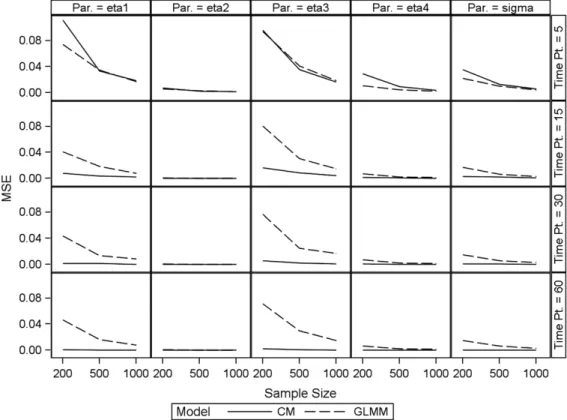
for the combined model.

Generally, the simulation results establish appropriate behavior of the models. Unsurprisingly, bias and MSE increase with decreasing sample size; this is true for all fixed effects, but not to the same extent for the variance component associated with the random effect. Bias and MSE favor the combined model. This superior behavior of the combined model is more pronounced for higher numbers of measurements per subject. It is interesting to note that these results hold in spite of the fact that data were generated under the GLMM. So, while strictly speaking the combined model is not necessary, it does perform well in alleviating the bias present in the GLMM-based estimators. In line with general likelihood theory, both estimators perform very well for large sample sizes. This is further shown through declining MSE values with increasing sample sizes inFig. 1, for various simulation conditions (seeFig. 2).

It is worth stating that even though the combined model demonstrated the ability to fit the data more efficiently, its numerical behavior is less straightforward than in the GLMM case. FromTable 5, we show the number of simulation runs

Table 3

Results of the GLMM and combined model based on 500 simulations.

True parameters GLMM Combined model

1.5 −0.5 −2 1 1.22 1.5 −0.5 −2 1 1.22 – Sample Size Measure ξ1 ξ2 ξ3 ξ4

√

d ξ1 ξ2 ξ3 ξ4

√

d C=β_α

For 5 time points

200 Estimate 1.4720 −0.4970 −2.0220 1.0098 1.2155 1.5790 −0.5186 −2.0663 1.0720 1.2738 0.0187 Std. error 0.2874 0.0793 0.3126 0.1045 0.1490 0.3735 0.0910 0.3493 0.1781 0.1546 0.0364 SB std. err. 0.2708 0.0772 0.3052 0.1027 0.1489 0.3244 0.0836 0.3029 0.1546 0.1809 0.0247 Bias −0.0280 0.0030 −0.0220 0.0098 −0.0045 0.0790 −0.0186 −0.0663 0.0720 0.0538 – Rel. bias −0.0187 0.0110 −0.0060 0.0098 −0.0037 0.0527 0.0371 0.0331 0.0720 0.0441 – MSE 0.0741 0.0060 0.0936 0.0106 0.0222 0.1115 0.0073 0.0961 0.0291 0.0356 – 500 Estimate 1.5034 −0.5036 −2.0116 1.0048 1.2123 1.5450 −0.5076 −2.0400 1.0389 1.2430 0.0110 Std. error 0.1817 0.0501 0.1967 0.0657 0.0937 0.2256 0.0553 0.2113 0.1059 0.0912 0.0222 SB std. err. 0.1866 0.0513 0.2013 0.0663 0.0998 0.1767 0.0474 0.1833 0.0879 0.1107 0.0149 Bias 0.0034 −0.0036 −0.0116 0.0048 −0.0077 0.0450 −0.0076 −0.0400 0.0389 0.0230 – Rel. bias 0.0022 0.0058 0.0072 0.0048 −0.0063 0.0300 0.0151 0.0200 0.0389 0.0189 – MSE 0.0348 0.0026 0.0407 0.0044 0.0100 0.0332 0.0023 0.0352 0.0092 0.0128 – 1000 Estimate 1.5123 −0.5030 −2.0056 1.0009 1.2181 1.5331 −0.5060 −2.0196 1.0189 1.2378 0.0064 Std. error 0.1286 0.0354 0.1390 0.0463 0.0662 0.1548 0.0383 0.1423 0.0709 0.0569 0.0148 SB std. err. 0.1289 0.0363 0.1367 0.0456 0.0652 0.1324 0.0348 0.1269 0.0578 0.0730 0.0099 Bias 0.0123 −0.0030 −0.0056 0.0009 −0.0019 0.0331 −0.0060 −0.0196 0.0189 0.0178 – Rel. bias 0.0082 0.0028 0.0060 0.0009 −0.0016 0.0221 0.0120 0.0098 0.0189 0.0146 – MSE 0.0168 0.0013 0.0187 0.0021 0.0043 0.0186 0.0012 0.0165 0.0037 0.0056 – For 15 time points

200 Estimate 1.4857 −0.5005 −2.0348 1.0096 1.2133 1.5002 −0.4999 −2.0106 1.0052 1.2189 0.0002 Std. error 0.2062 0.0313 0.2747 0.0794 0.1229 0.2275 0.0333 0.3247 0.1177 0.1238 0.0135 SB std. err. 0.2013 0.0320 0.2814 0.0855 0.1303 0.0889 0.0149 0.1268 0.0414 0.0546 0.0005 Bias −0.0143 −0.0005 −0.0348 0.0096 −0.0067 0.0002 0.0001 −0.0106 0.0052 −0.0011 – Rel. bias −0.0095 0.0174 0.0010 0.0096 −0.0055 0.0001 −0.0001 0.0053 0.0052 −0.0009 – MSE 0.0407 0.0010 0.0804 0.0074 0.0170 0.0079 0.0002 0.0162 0.0017 0.0030 – 500 Estimate 1.5041 −0.5012 −2.0045 0.9997 1.2109 1.5010 −0.5001 −2.0091 1.0036 1.2177 0.0001 Std. error 0.1302 0.0198 0.1725 0.0497 0.0774 0.1318 0.0198 0.1897 0.0611 0.0735 0.0032 SB std. err. 0.1368 0.0200 0.1747 0.0486 0.0805 0.0574 0.0095 0.0918 0.0294 0.0450 0.0002 Bias 0.0041 −0.0012 −0.0045 −0.0003 −0.0091 0.0010 −0.0001 −0.0091 0.0036 −0.0023 – Rel. bias 0.0028 0.0023 0.0024 −0.0003 −0.0074 0.0006 0.0003 0.0046 0.0036 −0.0019 – MSE 0.0187 0.0004 0.0305 0.0024 0.0066 0.0033 0.0001 0.0085 0.0009 0.0020 – 1000 Estimate 1.4978 −0.5001 −2.0042 1.0007 1.2175 1.5002 −0.5002 −2.0003 1.0004 1.2220 0.0001 Std. error 0.0921 0.0139 0.1222 0.0352 0.0548 0.0928 0.0140 0.1345 0.0411 0.0522 0.0015 SB std. err. 0.0901 0.0138 0.1230 0.0364 0.0561 0.0474 0.0078 0.0654 0.0200 0.0330 0.0001 Bias −0.0022 −0.0001 −0.0042 0.0007 −0.0025 0.0002 −0.0002 −0.0003 0.0004 0.0020 – Rel. bias −0.0014 0.0021 0.0001 0.0007 −0.0020 0.0001 0.0004 0.0002 0.0004 0.0016 – MSE 0.0081 0.0002 0.0151 0.0013 0.0032 0.0022 0.0001 0.0043 0.0004 0.0011 –

performed to obtain the required 500 simulated results for the two models. It was observed that the proportion of converging sets is lower in the combined model than in the GLMM model. This can be attributed to sensitivity to the starting values. In practice, this points to the need for carefully selecting starting values (seeFig. 3).

7.2. Binomial-type models for binomial data with logit link

Here, we turn to the behavior of GLMM and the combined model for binomial data. A modified version of the settings in the previous section was adopted. We assume for an independent subjectiat occasionjthatkrepeated Bernoulli trials are conducted. We generated the responseZijby randomly samplingmijwhich we assume to follow a normal distribution, N

(

10

,

4

)

. The choice of the mean and variance for generating themij’s was guided by the fact that with large values, the model takes longer to converge. Also, we avoided the occurrence of large-valued factorials. The true model parameters were as in the previous section. Themij’s were approximated to the nearest integer and used together with the predicted probability generated from the transformed sum of the predictors and the random effect to predict the number of successes. The model used to generate the data differs from(38)only by replacing the distribution ofYij

|

biwithZij

|

bi

∼

Bin

(

mij

, π

ij

)

. The same ranges for the sample sizeNand number of time pointsnwere considered. For each parameter setting, 200 simulations were conducted. Due to the complexity of the partially marginalized log-likelihood, the coding required somewhat more effort than in the binary case. The Newton–Raphson optimization algorithm was selected to maximize the full marginal likelihood function with 50 quadrature nodes. Results are presented inTables 6and7. The constraint

αβ

=

1 is applied to ensure identifiability.

104 G. Molenberghs et al. / Journal of Multivariate Analysis 111 (2012) 94–109 Table 4

Results of the GLMM and combined model based on 500 simulations.

True parameters GLMM Combined model

1.5 −0.5 −2 1 1.22 1.5 −0.5 −2 1 1.22 – Sample Size Measure ξ1 ξ2 ξ3 ξ4

√

d ξ1 ξ2 ξ3 ξ4

√

d C=β_α

For 30 time points

200 Estimate 1.5025 −0.5012 −1.9974 1.0016 1.2166 1.4978 −0.4996 −2.0007 0.9999 1.2190 0.0000 Std. error 0.2030 0.0298 0.2738 0.0790 0.1227 0.2231 0.0323 0.3318 0.1300 0.1442 0.0125 SB std. err. 0.2097 0.0304 0.2769 0.0837 0.1208 0.0423 0.0074 0.0747 0.0281 0.0250 0.0001 Bias 0.0025 −0.0012 0.0026 0.0016 −0.0034 −0.0022 0.0004 −0.0007 −0.0001 −0.0010 – Rel. bias 0.0016 −0.0013 0.0023 0.0016 −0.0028 −0.0015 −0.0007 0.0004 −0.0001 −0.0008 – MSE 0.0440 0.0009 0.0767 0.0070 0.0146 0.0018 0.0001 0.0056 0.0008 0.0006 – 500 Estimate 1.5055 −0.5011 −2.0127 1.0050 1.2193 1.5018 −0.5003 −2.0016 1.0009 1.2190 0.0000 Std. error 0.1283 0.0188 0.1733 0.0500 0.0774 0.1320 0.0193 0.1876 0.0641 0.0814 0.0045 SB std. err. 0.1174 0.0187 0.1577 0.0484 0.0749 0.0370 0.0066 0.0446 0.0136 0.0289 0.0000 Bias 0.0055 −0.0011 −0.0127 0.0050 −0.0007 0.0018 −0.0003 −0.0016 0.0009 −0.0010 – Rel. bias 0.0037 0.0063 0.0022 0.0050 −0.0006 0.0012 0.0006 0.0008 0.0009 −0.0008 – MSE 0.0138 0.0004 0.0250 0.0024 0.0056 0.0014 0.0000 0.0020 0.0002 0.0008 – 1000 Estimate 1.5039 −0.5003 −2.0010 0.9997 1.2165 1.5010 −0.4999 −1.9976 1.0000 1.2182 0.0000 Std. error 0.0905 0.0133 0.1220 0.0351 0.0546 0.0912 0.0134 0.1287 0.0407 0.0558 0.0015 SB std. err. 0.0919 0.0124 0.1296 0.0344 0.0550 0.0171 0.0042 0.0310 0.0101 0.0203 0.0000 Bias 0.0039 −0.0003 −0.001 −0.0003 −0.0035 0.0010 0.0001 0.0024 0.0000 −0.0018 – Rel. bias 0.0026 0.0005 0.0006 −0.0003 −0.0029 0.0006 −0.0001 −0.0012 0.0000 −0.0014 – MSE 0.0085 0.0002 0.0168 0.0012 0.0030 0.0003 0.0000 0.0010 0.0001 0.0004 – For 60 time points

200 Estimate 1.4954 −0.5015 −2.0157 1.0091 1.2188 1.4972 −0.4999 −2.0017 1.0002 1.2199 0.0000 Std. error 0.2032 0.0299 0.2748 0.0796 0.1228 0.2146 0.0313 0.3334 0.1278 0.1403 0.0099 SB std. err. 0.2157 0.0303 0.2669 0.0796 0.1208 0.0326 0.0052 0.0431 0.0133 0.0145 0.0000 Bias −0.0046 −0.0015 −0.0157 0.0091 −0.0012 −0.0028 0.0001 −0.0017 0.0002 −0.0001 – Rel. bias −0.0031 0.0078 0.0030 0.0091 −0.0009 −0.0019 −0.0003 0.0008 0.0002 −0.0001 – MSE 0.0465 0.0009 0.0715 0.0064 0.0146 0.0011 0.0000 0.0019 0.0002 0.0002 – 500 Estimate 1.4961 −0.5008 −2.0169 1.0046 1.2138 1.5002 −0.5001 −2.0015 1.0003 1.2207 0.0000 Std. error 0.1280 0.0189 0.1730 0.0499 0.0773 0.1320 0.0193 0.1925 0.0670 0.0825 0.0043 SB std. err. 0.1269 0.0189 0.1710 0.0487 0.0784 0.0106 0.0027 0.0265 0.0074 0.0154 0.0000 Bias −0.0039 −0.0008 −0.0169 0.0046 −0.0062 0.0002 −0.0001 −0.0015 0.0003 0.0007 – Rel. bias −0.0026 0.0085 0.0016 0.0046 −0.0051 0.0001 0.0003 0.0008 0.0003 0.0005 – MSE 0.0161 0.0004 0.0295 0.0024 0.0062 0.0001 0.0000 0.0007 0.0001 0.0002 – 1000 Estimate 1.5014 −0.5007 −1.9965 1.0002 1.2189 1.5008 −0.5001 −1.9998 1.0000 1.2208 0.0000 Std. error 0.0906 0.0133 0.1221 0.0352 0.0547 0.0931 0.0136 0.1323 0.0439 0.0574 0.0023 SB std. err. 0.0901 0.0134 0.1213 0.0359 0.0558 0.0141 0.0023 0.0184 0.0080 0.0108 0.0000 Bias 0.0014 −0.0007 0.0035 0.0002 −0.0011 0.0008 −0.0001 0.0002 0.0000 0.0008 – Rel. bias 0.0010 −0.0017 0.0013 0.0002 −0.0009 0.0006 0.0002 −0.0001 0.0000 0.0006 – MSE 0.0081 0.0002 0.0147 0.0013 0.0031 0.0002 0.0000 0.0003 0.0001 0.0001 – Table 5

Simulation study. Convergence rate for binary data.

Time points Sample size GLMM Combined model Runs Rate (%) Runs Rate (%) 5 200 500 100.00 756 66.14 500 500 100.00 620 80.65 1000 500 100.00 562 88.97 15 200 500 100.00 818 61.12 500 505 99.01 735 68.03 1000 503 99.40 645 77.52 30 200 501 99.80 619 80.78 500 502 99.60 548 91.24 1000 503 99.40 524 95.42 60 200 500 100.00 698 71.63 500 502 99.60 542 92.25 1000 504 99.21 525 95.24

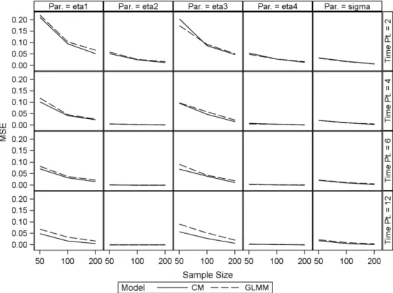
The results for the two models show that parameter estimates have very small bias for each of the simulations, underscoring good performance of both methods. They are difficult to tell apart in bias terms (seeFig. 4). Based on the MSE values, the combined model seems to work well, especially when the number of measurements per subject is high.

Fig. 1. Plot of MSE against sample size for the GLMM and combined model (binary outcomes).

106 G. Molenberghs et al. / Journal of Multivariate Analysis 111 (2012) 94–109

Fig. 3. Plot of MSE against sample size for the GLMM and combined model (binomial outcomes).

Table 6

Simulation study. Results of the GLMM and combined model based on 200 simulations.

True parameters GLMM Combined model

1.5 −0.5 −2 1 1.22 1.5 −0.5 −2 1 1.22 – Sample size Measure ξ1 ξ2 ξ3 ξ4

√

d ξ1 ξ2 ξ3 ξ4

√

d β=1/α For 2 time points

50 Estimate −1.5074 0.5160 −2.0142 1.0004 1.1818 −1.4799 0.5306 −2.0283 1.0387 1.2027 0.09116 Std. error 0.4413 0.2285 0.4437 0.2302 0.1659 0.4573 0.2389 0.4596 0.2467 0.1898 0.20848 SB std. err. 0.4703 0.2432 0.4182 0.2226 0.1750 0.4589 0.2260 0.4512 0.2319 0.1846 0.10975 Bias −0.0074 0.0160 −0.0142 0.0004 −0.0382 0.0201 0.0306 −0.0283 0.0387 −0.0173 – Rel. bias 0.0049 0.0319 0.0071 0.0004 −0.0313 −0.0134 0.0612 0.0141 0.0387 −0.0142 – MSE 0.2212 0.0594 0.1751 0.0496 0.0321 0.2110 0.0520 0.2044 0.0553 0.0344 – 100 Estimate −1.5404 0.5113 −1.9674 0.9852 1.1970 −1.5283 0.5294 −1.9885 1.0278 1.2314 0.08467 Std. error 0.3114 0.1607 0.3130 0.1618 0.1182 0.6228 0.3939 0.3232 0.1778 0.1287 0.13566 SB std. err. 0.3185 0.1651 0.3034 0.1673 0.1262 0.3064 0.1574 0.2939 0.1650 0.1334 0.10429 Bias −0.0404 0.0113 0.0326 −0.0148 −0.0230 −0.0283 0.0294 0.0115 0.0278 0.0114 – Rel. bias 0.0269 0.0227 −0.0163 −0.0148 −0.0188 0.0189 0.0589 −0.0058 0.0278 0.0094 – MSE 0.1031 0.0274 0.0931 0.0282 0.0165 0.0947 0.0256 0.0865 0.0280 0.0179 – 200 Estimate −1.5195 0.5057 −2.0134 1.0003 −1.5195 −1.5205 0.5186 −2.0023 1.0076 1.2310 0.07996 Std. error 0.2214 0.1139 0.2217 0.1140 0.2214 0.2285 0.1175 0.2283 0.1215 0.0907 0.11902 SB std. err. 0.2580 0.1277 0.2273 0.1296 0.2580 0.2282 0.1108 0.2169 0.1192 0.0854 0.09044 Bias −0.0195 0.0057 −0.0134 0.0003 −0.0195 −0.0205 0.0186 −0.0023 0.0076 0.0110 – Rel. bias 0.0130 0.0114 0.0067 0.0003 0.0130 0.0137 0.0372 0.0012 0.0076 0.0090 – MSE 0.0669 0.0163 0.0518 0.0168 0.0669 0.0525 0.0126 0.0471 0.0143 0.0074 – For 4 time points

50 Estimate −1.4579 0.4908 −2.0402 1.0077 1.1806 −1.4722 0.4995 −2.0515 1.0248 1.2064 0.04906 Std. error 0.3098 0.0716 0.3187 0.0838 0.1417 0.3160 0.0733 0.7798 0.1519 0.1703 0.09821 SB std. err. 0.3420 0.0789 0.3095 0.0785 0.1398 0.3182 0.0707 0.3061 0.0888 0.1433 0.05985 Bias 0.0421 −0.0092 −0.0402 0.0077 −0.0394 0.0278 −0.0005 −0.0515 0.0248 −0.0136 – Rel. bias −0.0281 −0.0183 0.0201 0.0077 −0.0323 −0.0185 −0.0009 0.0257 0.0248 −0.0111 – MSE 0.1187 0.0063 0.0974 0.0062 0.0211 0.1020 0.0050 0.0963 0.0085 0.0207 – 100 Estimate −1.5307 0.5051 −2.0085 1.0016 1.2052 −1.5314 0.5061 −1.9853 1.0095 1.2105 0.04452 Std. error 0.2218 0.0507 0.2270 0.0589 0.1019 0.2202 0.0510 0.3549 0.0693 0.1032 0.08172 SB std. err. 0.2117 0.0536 0.2411 0.0635 0.0993 0.2013 0.0474 0.2185 0.0644 0.1070 0.04957 Bias −0.0307 0.0051 −0.0085 0.0016 −0.0148 −0.0314 0.0061 0.0147 0.0095 −0.0095 – Rel. bias 0.0205 0.0102 0.0042 0.0016 −0.0122 0.0209 0.0121 −0.0073 0.0095 −0.0078 – MSE 0.0458 0.0029 0.0582 0.0040 0.0101 0.0415 0.0023 0.0480 0.0042 0.0115 – 200 Estimate −1.5253 0.5021 −2.0084 1.0009 −1.5253 −1.4977 0.5014 −2.0185 1.0137 1.2270 0.02935 Std. error 0.1572 0.0358 0.1609 0.0416 0.1572 0.3621 0.0884 0.2327 0.0786 0.0693 0.06100 SB std. err. 0.1605 0.0344 0.1510 0.0393 0.1605 0.1478 0.0340 0.1205 0.0359 0.0514 0.03438 Bias −0.0253 0.0021 −0.0084 0.0009 −0.0253 0.0023 0.0014 −0.0185 0.0137 0.0070 – Rel. bias 0.0168 0.0043 0.0042 0.0009 0.0168 −0.0015 0.0028 0.0093 0.0137 0.0058 – MSE 0.0264 0.0012 0.0229 0.0015 0.0264 0.0219 0.0012 0.0149 0.0015 0.0027 –

In spite of these advantages of the combined model, and in line with the binary case, also here numerical stability can be an issue. We see from the results inTable 8that the fitting becomes more difficult when sample sizes are increased. We however maintain that with appropriate choice of starting values, this can be overcome.

8. Concluding remarks

In the spirit of MVD and MVDV, we have proposed a model combining normal and non-normal random effects, to handle hierarchical binary data that are subject to both overdispersion and correlation. The non-normal random effects typically take a beta form, inspired by the conjugate nature of data relative to the Bernoulli model. The resulting model is thus of a logistic-normal-beta form. Also the probit-normal-beta model has been given attention. Unlike the aforementioned papers, we explicitly allow for repeated, overdispersed binomial data. The singular feature in binary data that overdispersion cannot be identified from univariate outcomes does not occur with binomial data. The latter are, therefore, more in line with developments for count data and time-to-event outcomes.

Special cases of our model are the beta-binomial model on the one hand and the GLMM on the other. The GLMM in this case would typically take a logistic-normal form. The logit link, though, is specific in the sense that it does not allow for closed-form marginalization, as indicated in MVDV, neither for the joint distribution, nor for mean, variance, and higher moments. While the model can still be fitted without trouble using standard software, using so-called analytical–numerical integration, it is sometimes desirable to have closed forms nevertheless. This is why we also focused on the probit link, producing the probit-normal-beta model. In that case, the combined model, and all of its special cases, does allow for such closed forms. Using the probit-logit relationship, the probit version can be exploited to closely approximate the logit case.

108 G. Molenberghs et al. / Journal of Multivariate Analysis 111 (2012) 94–109 Table 7

Simulation study. Results of the GLMM and combined model based on 200 simulations.

True parameters GLMM Combined model

1.5 −0.5 −2 1 1.22 1.5 −0.5 −2 1 1.22 – Sample size Measure ξ1 ξ2 ξ3 ξ4

√

d ξ1 ξ2 ξ3 ξ4

√

d β=1/α For 6 time points

50 Estimate −1.4846 0.4998 −2.0175 1.0025 1.1740 −1.4675 0.4993 −1.9878 1.0172 1.1902 0.03454 Std. error 0.2805 0.0408 0.2947 0.0602 0.1353 1.3998 0.2076 0.2990 0.0678 0.1377 0.05960 SB std. error 0.2866 0.0386 0.3005 0.0603 0.1415 0.2644 0.0369 0.2608 0.0645 0.1391 0.03713 Bias 0.0154 −0.0002 −0.0175 0.0025 −0.0460 0.0325 −0.0007 0.0122 0.0172 −0.0298 – Rel. bias −0.0103 −0.0004 0.0088 0.0025 −0.0377 −0.0217 −0.0013 −0.0061 0.0172 −0.0245 – MSE 0.0824 0.0015 0.0906 0.0036 0.0221 0.0710 0.0014 0.0682 0.0045 0.0202 – 100 Estimate −1.5072 0.4974 −1.9929 0.9977 1.1940 −1.5241 0.5037 −1.9995 1.0105 1.2119 0.02389 Std. error 0.2008 0.0288 0.2104 0.0424 0.0971 0.1996 0.0294 0.2107 0.0474 0.0992 0.04874 SB std. error 0.1928 0.0270 0.2075 0.0404 0.1047 0.1751 0.0275 0.1992 0.0410 0.0965 0.02629 Bias −0.0072 −0.0026 0.0071 −0.0023 −0.0260 −0.0241 0.0037 0.0005 0.0105 −0.0081 – Rel. bias 0.0048 −0.0053 −0.0035 −0.0023 −0.0213 0.0161 0.0074 −0.0003 0.0105 −0.0066 – MSE 0.0372 0.0007 0.0431 0.0016 0.0116 0.0312 0.0008 0.0397 0.0018 0.0094 – 200 Estimate −1.5102 0.4985 −2.0049 1.0016 −1.5102 −1.5181 0.5036 −2.0087 1.0083 1.2125 0.02032 Std. error 0.1436 0.0204 0.1502 0.0300 0.1436 2.3446 0.1733 0.1517 0.0325 0.0760 0.04757 SB std. error 0.1488 0.0203 0.1389 0.0307 0.1488 0.1210 0.0169 0.1091 0.0267 0.0543 0.02125 Bias −0.0102 −0.0015 −0.0049 0.0016 −0.0102 −0.0181 0.0036 −0.0087 0.0083 −0.0075 – Rel. bias 0.0068 −0.0029 0.0024 0.0016 0.0068 0.0121 0.0073 0.0044 0.0083 −0.0061 – MSE 0.0222 0.0004 0.0193 0.0009 0.0222 0.0150 0.0003 0.0120 0.0008 0.0030 – For 12 time points

50 Estimate −1.4921 0.5014 −2.0272 1.0063 1.1764 −1.4728 0.5017 −2.0362 1.0137 1.1926 0.00974 Std. error 0.2619 0.0220 0.2872 0.0527 0.1333 0.2664 0.0230 0.2923 0.0555 0.1403 0.01673 SB std. error 0.2621 0.0210 0.3004 0.0525 0.1454 0.2203 0.0206 0.2373 0.0510 0.1307 0.01260 Bias 0.0079 0.0014 −0.0272 0.0063 −0.0436 0.0272 0.0017 −0.0362 0.0137 −0.0274 – Rel. bias −0.0053 0.0027 0.0136 0.0063 −0.0358 −0.0181 0.0035 0.0181 0.0137 −0.0224 – MSE 0.0688 0.0004 0.0910 0.0028 0.0230 0.0493 0.0004 0.0576 0.0028 0.0178 – 100 Estimate −1.5189 0.5007 −2.0157 1.0034 1.1976 −1.5154 0.5013 −2.0139 1.0060 1.1994 0.00849 Std. error 0.1877 0.0154 0.2053 0.0371 0.0956 0.3693 0.0179 0.1988 0.0369 0.0929 0.01520 SB std. error 0.1833 0.0150 0.2261 0.0399 0.0957 0.1217 0.0128 0.1541 0.0302 0.0679 0.00836 Bias −0.0189 0.0007 −0.0157 0.0034 −0.0224 −0.0154 0.0013 −0.0139 0.0060 −0.0206 – Rel. bias 0.0126 0.0014 0.0078 0.0034 −0.0184 0.0103 0.0025 0.0070 0.0060 −0.0169 – MSE 0.0340 0.0002 0.0514 0.0016 0.0097 0.0150 0.0002 0.0239 0.0009 0.0050 – 200 Estimate −1.5153 0.5000 −2.0080 0.9984 −1.5153 −1.5076 0.5010 −2.0010 1.0030 1.2112 0.00799 Std. error 0.1340 0.0109 0.1462 0.0260 0.1340 0.1343 0.0110 0.1472 0.0270 0.0694 0.01227 SB std. error 0.1313 0.0122 0.1446 0.0269 0.1313 0.0798 0.0084 0.0807 0.0171 0.0456 0.00596 Bias −0.0153 0.0000 −0.0080 −0.0016 −0.0153 −0.0076 0.0010 −0.0010 0.0030 −0.0088 – Rel. bias 0.0102 0.0001 0.0040 −0.0016 0.0102 0.0051 0.0019 0.0005 0.0030 −0.0072 – MSE 0.0175 0.0001 0.0210 0.0007 0.0175 0.0064 0.0001 0.0065 0.0003 0.0022 – Table 8

Simulation study. Convergence rates for binomial data.

Time points Sample size GLMM Combined model Runs Rate (%) Runs Rate (%) 2 50 200 100 291 68.73 100 200 100 318 62.89 200 200 100 395 50.63 4 50 200 100 377 53.05 100 200 100 599 33.39 200 200 100 1147 17.44 6 50 200 100 500 40.00 100 200 100 878 22.78 200 200 100 3407 5.87 12 50 200 100 806 24.81 100 200 100 1581 12.65 200 200 100 8276 2.42

Our modeling approach may appear to be relatively complex. However, the needs of the application at hand may justify its use. Moreover, the fact that both the logistic-normal and probit-normal generalized linear mixed models on the one hand and the beta-binomial model on the other follow as special cases are a strong asset.

The unique position of the logistic-normal-beta model is also seen through the fact that it does not enjoy so-called strong conjugacy, in spite of the conjugacy in the beta-binomial case. Even though strong conjugacy does not apply to the probit-normal-beta case neither, the latter model does enjoy desirable analytical properties, as mentioned before.

Two sets of data were analyzed. The first one exhibited a repeated-measures structure and was of a binary outcome type; the second one was of a binomial type, but without a repeated measures structure. It was not a surprise that the simultaneous identification of overdispersion and correlation in the binary case was difficult, even though the estimation of fixed-effects parameters is not affected by it. A limited simulation study, in both the binary and binomial cases, was conducted to examine the behavior of the combined models relative to their more conventional GLMM counterparts. Somewhat surprisingly, even when the data generating mechanism starts from a GLMM formulation, the combined model still exhibits better behavior, because it alleviates the typical small-sample maximum likelihood bias. For increasing sample sizes, the two showed similar behavior. While not studied in detail, it is evident that when the GLMM formulation is not adequate, the combined model will exhibit superior performance.

Programs and outputs can be found at web sitewww.ibiostat.be/software.

Acknowledgments

Financial support from the IAP research network #P6/03 of the Belgian Government (Belgian Science Policy) is gratefully acknowledged. This work was partially supported by a grant from Conselho Nacional de Desenvolvimento Científico e Tecnologia—CNPq, a Brazilian science funding agency.

Appendix. Supplementary data

Supplementary material related to this article can be found online athttp://dx.doi.org/10.1016/j.jmva.2012.05.005.

References

[1] A. Agresti, Categorical Data Analysis, second ed., John Wiley & Sons, New York, 2002.

[2] N.E. Breslow, D.G. Clayton, Approximate inference in generalized linear mixed models, Journal of the American Statistical Association 88 (1993) 9–25. [3] D.R. Cox, D.V. Hinkley, Theoretical Statistics, Chapman & Hall/CRC, London, 1974.

[4] M. De Backer, P. De Keyser, C. De Vroey, E. Lesaffre, A 12-week treatment for dermatophyte toe onychomycosis: terbinafine 250 mg/day vs. itraconazole 200 mg/day—a double-blind comparative trial, British Journal of Dermatology 134 (1996) 16–17.

[5] B. Engel, A. Keen, A simple approach for the analysis of generalized linear mixed models, Statistica Neerlandica 48 (1994) 1–22. [6] R.D. Gibbons, D. Hedeker, Random effects probit and logistic regression models for three-level data, Biometrics 53 (1997) 1527–1537. [7] D.K. Guilkey, J.L. Murphy, Estimation and testing in the random effects probit model, Journal of Econometrics 59 (1993) 301–317. [8] D. Hedeker, R.D. Gibbons, A random-effects ordinal regression model for multilevel analysis, Biometrics 51 (1994) 933–944. [9] J. Hinde, C.G.B. Demétrio, Overdispersion: models and estimation, Computational Statistics and Data Analysis 27 (1998) 151–170. [10] J. Hinde, C.G.B. Demétrio, Overdispersion: Models and Estimation, XIII Sinape, São Paulo, 1998.

[11] N.L. Johnson, S. Kotz, Distributions in Statistics, Continuous Univariate Distributions, Vol. 2, Houghton-Mifflin, Boston, 1970. [12] B. Jørgensen, Exponential dispersion models, Journal of the Royal Statistical Society, Series B 49 (1987) 127–162.

[13] J. Kleinman, Proportions with extraneous variance: single and independent samples, Journal of the American Statistical Association 68 (1973) 46–54. [14] Y. Lee, J.A. Nelder, Y. Pawitan, Generalized Linear Models with Random Effects: Unified Analysis viaH-likelihood., Chapman & Hall/CRC,