Online Load Balancing for MapReduce with
Skewed Data Input
Yanfang Le†, Jiangchuan Liu†, Funda Erg¨un‡, Dan Wang∗
† Simon Fraser University, BC, Canada, Email: {yanfangl, jcliu}@cs.sfu.ca ‡Indiana University Bloomington, Indiana, USA, Email: [email protected] ∗ The Hong Kong Polytechnic University, Hong Kong, Email: [email protected]
Abstract—MapReduce has emerged as a powerful tool for distributed and scalable processing of voluminous data. In this paper, we, for the first time, examine the problem of accommodat-ing data skew in MapReduce with online operations. Different from earlier heuristics in the very late reduce stage or after seeing all the data, we address the skew from the beginning of data input, and make no assumption about a priori knowledge of the data distribution nor require synchronized operations. We examine the input in a continuous fashion and adaptively assign tasks with a load-balanced strategy. We show that the optimal strategy is a constrained version of online minimum makespan and, in the MapReduce context where pairs with identical keys must be scheduled to the same machine, there is an online algorithm with a provable2-competitive ratio. We further suggest a sample-based enhancement, which, probabilistically, achieves a 3/2-competitive ratio with a bounded error.
I. INTRODUCTION
With the rapid growth of information in such applications as social networking and bioinformatics, there is an urgent need for large-scale data analysis and processing. With recent advances in Cloud Computing, MapReduce has emerged as a powerful tool for distributed and scalable processing of voluminous data [1]. The standard MapReduce framework consists of two steps [2], namely, Map and Reduce. In the Map phase, a master node takes the input, divides it into smaller sub-problems, and distributes them to worker nodes. A worker node processes the smaller problem, and passes the answer back to its master node. In the Reduce phase, the master node collects the answers to all the sub-problems and combines them to form the output for the original problem. This divide-and-conquer process enables MapReduce to work on huge datasets with distributed server clusters. Yet a user of MapReduce only needs to write the map and the reduce functions, which effectively hides the operation details of large server clusters, offering a highly flexible, scalable, and fault tolerant solution for general big data processing applications. The generic and simple interface also implies that MapRe-duce can be a bottleneck in the overall processing with specific applications or specific data. Significant efforts have been demonstrated on relieving blocking operations [3], improving energy efficiency [4], [5], enhancing scheduling [6], [7], or relaxing the single fixed dataflow [8], [9], [10], [11]. There
Funda Erg¨un‡is also with Simon Fraser University, BC, Canada. Dan Wang∗is also with The Hong Kong Polytechnic University Shenzhen Research Institute, Shenzhen, China.
have also been recent works on efficient scheduling of massive MapReduce jobs running in parallel [12], [13], [14]. Most of these studies have assumed that the input data are of uniform distribution, which, often being hashed to reduce worker nodes, naturally leads to a desirable balanced load in the later stages.
The real world data, however, are not necessarily uniform, and often exhibit remarkable skew. For example, in PageRank, the graph commonly includes nodes with much higher degrees of incoming edges than others [15], and in Inverted Index, cer-tain content can appear in many more documents than others [16]. Such skewed distribution of the input or intermediate data can make a small number of mappers or reducers take a significantly longer time to complete than others [17]. Recent experimental studies [15], [17], [16] have shown that, in the CloudBurst application with a biology dataset of a bimodal distribution, the slowest map task takes five times as long to complete as the fastest; PageRank with the Cloud9 data is even worse, where the slowest map task takes twice as long to complete as the second slowest, and the latter remains five times slower than the average. Our experiments with the WordCount application also show similar phenomena. Given that the overall finishing time is bounded by the slowest task, it can be dramatically prolonged with such skewed data.
In distributed databases, data skew is a known common phenomenon and there have been such mature solutions as joining, grouping, aggregation, and etc. [18], [19]. Unfortu-nately, these can hardly be applied in the MapReduce context. The map function transfers the input raw data into (key, value) pairs, and the reduce function merges all intermediate values associated with the same intermediate key. In the database case, the pairs sharing the same key are not necessary to be processed in a single machine; MapReduce, on the other hand, must guarantee that these pairs belong to the same partition, in other words, be distributed into the same reducer.
There have been pioneer works dealing with the data skew in MapReduce [20], [16], [21]. Most of them are offline heuristics, either waiting for all the mappers to finish so as to obtain the key frequencies, or sampling before the map tasks to estimate the data distribution and then partitioning in advance, or repartitioning the reduce tasks to balance the load among servers. These solutions can be time-consuming with excessive I/O costs or network overheads. They also lack theoretical bounds for the solutions given that most of them
are heuristics.
In this paper, we, for the first time, examine the problem of accommodating data skew in MapReduce with online opera-tions. In contrast with earlier solutions in the very late reduce stage [16] or after seeing all the data [20], we address the skew from the very beginning of data input, and make no assumption about the a priori knowledge of the data distribution, nor require synchronized operations. We examine the keys in a continuous fashion and adaptively assign the tasks with a load-balanced strategy. We show that the optimal strategy
is a constrained version of the online minimum makespan
problem[22], and demonstrate that, in the MapReduce context where tasks with identical keys must be scheduled to the same machine, there is an online algorithm with a provable 2-competitive ratio. We further suggest that the online solution can be enhanced by a sample-based algorithm, which identifies the most frequent keys and assigns associated tasks in advance. We show that, probabilistically, it achieves a 3/2-competitive ratio with a bounded error.
We evaluate our algorithms on both synthetic data and a real public data set. Our simulation results show that, in practice, the maximum loads of our online and sample-based algorithms are close to that of the offline solutions, and are significantly lower than that with the naive hash function in MapReduce. They enjoy comparable computation times as the hash function, which are much shorter than those of the offline solutions.
The rest of the paper is structured as follows. Section II introduces the background and motivation. Section III presents the problem formulation with the online model. Section IV illustrates our online algorithm and derives the2-competitive ratio. The Sample-based algorithm is discussed in Section V. Section VI offers the results for performance evaluation. We discuss further enhancements in Section VII. We briefly review related work in Section VIII and finally conclude the paper in Section IX.
II. BACKGROUND ANDMOTIVATION
In this section, we present an overview of MapReduce and also discuss the skew issues therein that motivate our study.
The MapReduce libraries have been written in differ-ent programming languages. Taking Apache Hadoop (High-availability distributed object-oriented platform), one of the most popular free implementations, as an example. Hadoop is based on a master-worker architecture, where a master node makes scheduling decisions and multiple worker nodes run tasks dispatched from the master.
In the MapPhase, the master node divides a large dataset into small blocks and distributes them to the map workers. The map workers generate a large amount of intermediate (key, value) pairs and report the locations of these pairs on the local disk to the master, who is responsible for forwarding these locations to the reduce workers.
A hash function then assigns the values to different worker nodes to process in theReducePhase. In Hadoop, the default hash function is simply Hash(HashCode( intermediate key)
Ă ď ď Đ Đ Ě Ă Ă Ă Ğ Ĩ Ĩ Ě Ě Ő Ő Ă Ă Ă Ă Ă Ă Ă Ă Ő Ő Ő Ő Ĩ Ĩ
,ĂƐŚ Ă͗ϭϮ͖Ě͗ϯ͖Ő͗ϰ ď͗Ϯ͖Ğ͗ ϭ Đ͗Ϯ͖Ĩ͗ϰ
KƉƚŝŵĂů Ă͗ϭϮ ď͗Ϯ͖Ě͗ ϯ͖Ĩ͗ ϰ Đ͗Ϯ͖Ğ͗ϭ͖Ő͗ ϲ
Figure 1. An illustrative example for key assignment in MapReduce. There are three machines in this example. The “Hash”, “Optimal” rows represent the result load distribution of each scheduling, respectively.
mod ReducerNumber), which is highly efficient and naturally achieves load balance if the keys are uniformly distributed. This however can fail with skewed inputs. For example, in WordCount, a classical MapReduce application, popular words such as “the,” “a,” and “of” appear much more frequently, which, after hashing, impose heavier workloads to the corre-sponding reduce workers. Consider a toy example shown in Figure 1 with a skewed input. The naive hash function will assign keysa,dandgto the first machine, keysbandeto the second machine, and keys c and f to the third machine. As a result, the first machine achieves a maximum load with19, six times more than that of the least load, while the maximum load of the balanced solution would be 12 as shown in the “optimal” row. Since the overall finishing time is bounded by the slowest, such a simple hash-based scheduling is simply not satisfactory.
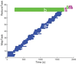
It is worth noting that Hadoop starts to execute theReduce phase before every corresponding partition is available, i.e., it is activated when only part of maps has been completed (5% by default) [16]. The rationale behind this synchronous operation is to overlap the map and reduce and consequently reduce the maximum finishing time; yet it can prevent from making a partition in advance. In fact, theReducephase further consists of three subphases: shuffle, in which the task pulls the map outputs;sort, in which the map outputs are sorted by keys; andreduce function executing, in which a user-defined function takes the map outputs with each key, and, after all the mappers finish working, starts to run and generates the final outputs. In Figure 2, we show a detailed measurement of processing times of all the phases for a WordCount application running on Amazon EC2. The Mapphase starts at time zero and then theReducephase, theshufflesubphase, starts at about 200s. We can see that the shuffle finishing time is much longer than the reduce function executing time, for the reduce workers should wait for the map workers to generate intermediate pairs while using remote procedure calls to read the buffered data from the local disks of the map workers. Also note that the maximum map finishing time is quite close to that of shuffle subphase. Therefore, if we wait until all the keys are generated, in other words, start the shufflesubphase after all the map workers finish, the overall job finishing time will be doubled. This is unfortunately what the state-of-the-art offline algorithms do for load balancing. It motivates our design for an online solution to start theshufflesubphase as soon as possible while making the maximum load of the reduce workers as low
0 500 1000 1500 2000 0 10 20 30 40 50 60 70 80 Time (s) MapTask ReduceTask
a
b
c
bc
Figure 2. We ran WordCount application on Amazon EC2 with4instances and we set70map tasks and7reduce tasks. This figure describes the timing flow of eachMaptask andReducetask. Regionarepresents the actual map function executing time. Regionbrepresents the shuffling time and region
crepresents the actual reduce function executing time. The regions between bothbandcrepresent the sorting time.
as possible.
III. PROBLEMDEFINITION
We consider a general scenario, where, during the Map
phase, the mapper nodes generate many intermediate values (data) with associated keys. Each of these, which we denote
as(ki, li), forms a (key, location) pair, where locationlirefers
to where the (key, value) pairs is stored, and the worker nodes report the pair to the master node1. For the rest of this paper, we will only be interested in processing the key attribute of such a pair, and sometimes, for simplicity, skip the location attribute altogether. The master node then assigns these pairs to different machines based on the key values. Each such pair must be assigned to one machine for processing, with the additional restriction that the pairs with the same key must be assigned to the same machine. The number of pairs assigned
to a machine makes up the load of the machine. Here, we
assume each machine will have a finishing time which is directly proportional to its load, and the finishing time of the machine with the highest load (called the makespan) will be the overall finishing time. The objective then is to minimize the overall finishing time by minimizing the maximum load of all the machines 2. From the perspective of the master node, the input is a streamS= (b1, b2,· · ·, bN)of lengthN, where eachbidenotes a (key, location) pair. LetNdenote the number of different keys; we denoteC={c1, c2,· · ·, cN}as
the universal set of the different keys, with bi∈C for every
i∈N.
1Note that the value isnotbeing reported, and thus, the information received
by the master node for each item will require a small amount of space.
2Here we make an implicit assumption that each pair represents a workload
of unit size, but our algorithm can easily work also for variable integer workload weights.
We assume that there arem identical machines numbered
1, . . . , m. We denote the load of machine i byMi, i.e., the
number of pairs assigned to machinei. Initially, all loads are 0. Our goal is to assign each bi in S to a machine, so as to obtain
min M ax
i∈{1,2,···,m}Mi
such that any two pairs(k1, l1)and (k2, l2)will be assigned to the same machine ifk1=k2.
We consider two input models, leading to two computational models. In our first model, we allow arbitrary (possibly adver-sarial) input, and stipulate that the master node will assign the pairs in a purely online fashion. In our second model, we assume that the input comes from a probability distribution, and, in order to exploit this fact, the master node is allowed to store and processsamplesof its input before starting to assign the samples and the rest of the pairs in an online fashion.
IV. A 2-COMPETITIVEFULLYONLINEALGORITHM
In order to minimize the overall finishing time, it makes sense to start the shuffle subphase as soon as possible, with
as much an overlap with the Map phase as possible. In
this section, we give an online algorithm, List-based Online Scheduling, for assigning the keys to the machines. Our algorithm decides, upon receiving a (key, location) pair, to which machine to assign that item without any knowledge of what other items may be received in the future. We assume that the stream of items can be arbitrary, that is, after our algorithm makes a particular assignment, it can possibly receive the “worst” stream of items for that assignment. Our algorithm will be analyzed for the worst case scenario: we will compare its effectiveness to that of the best offline algorithm, i.e., one that makes its decisions with the knowledge of the entire input. For assigning items to machines based on their keys, we adopt a Greedy-Balance load balancing approach [23] of assigning unassigned keys to the machine with the smallest load once they come in.
Algorithm 1List-based Online Scheduling
Read pair (ki,li) from S
ifki has been assigned to machinej then
Assign the pair to the machine j
else
Assign the pair to the machine with the least load
end if
We now show that this algorithm yields an overall finishing time which at most twice that of the best offline algorithm.
Theorem 1. List-based Online Scheduling has a competitive
ratio of 2.
Proof. Let OPT denote the offline optimum makespan, the
maximum finishing time. Assume machine j is the machine
with the longest finishing time in the optimal offline solution and T is the number of pairs read just before the last new key, saycj, is assigned to machinej. Obviously,T must be
Ă ď ď Đ Đ Ě Ă Ă Ă Ğ Ĩ Ĩ Ě Ě Ő Ő Ă Ă Ă Ă Ă Ă Ă Ă Ő Ő Ő Ő Ĩ Ĩ
KŶůŝŶĞ Ă͗ϭϮ͖Ě͗ϯ ď͗Ϯ͖Ğ͗ ϭ͖Ő͗ ϰ Đ͗Ϯ͖Ĩ͗ϰ
^ĂŵƉůĞͲďĂƐĞĚ Ă͗ϭϮ ď͗Ϯ͖Ě͗ ϯ͖Ĩ͗ ϰ Đ͗Ϯ͖Ğ͗ϭ͖Ő͗ ϲ
Figure 3. An illustrative example showing benefits of sampling. The setting is the same as in Figure 1. The “Online” and “Sample-based” rows represent the respective result load of each machine in the online and sample-based schedules.
less thanN, the total length of the input. Then, at that timecj is assigned to machine j,j must have had the smallest load, say Lj. Thus we have:
Lj≤ T
m <
N
m ≤OP T
Let |cj| denote the number of pairs with keycj in S. Then, the finishing time of machine j, denoted byT, which is also the makespan, is
T =Lj+|cj| ≤OP T +OP T = 2OP T
Thus, with our List-based Online algorithm, the makespan can achieve a 2-competitive ratio to the offline optimal makespan.
V. A SAMPLING-BASEDSEMI-ONLINEALGORITHM
Our previous algorithm made no assumptions about our advance knowledge of the key frequencies. Clearly, if we had some a priori knowledge about these frequencies, we could make the key assignments more efficiently.
In this section, we assume that the pairs are such that their keys are drawn independently from an unknown distribution. In order to exploit this, we compromise on the online nature of our algorithm and start by collecting a small number of input pairs into a samplebefore making any assignments. We then use this sample to estimate the frequencies of theKmost frequent keys in this distribution, and use this information later to process our stream in an online fashion. In order to observe the advantages of such a scheme, consider another toy example shown in Figure 3. If we can wait for a short period before making any assignments, for instance, collect the first 9keys in the example and assign the frequent keys to the machine with the least load in order of frequency, the maximum load is reduced to 12from 15.
Our algorithm classifies keys into two distinct groups: the
K most frequent, called heavy keys, and the remaining, less frequent keys. The intuition is that the heavy keys contribute much more strongly to the finishing time than the other keys, and thus, need to be handled more carefully. As a result, our algorithm performs assignments of the keys to the machines differently for the two groups.
We first consider how to identify the heavy keys. Clearly, if one could collect all of the stream S, the problem can be solved exactly and easily. However, this would use too much space and delay the assignment process. Instead, we would like
to trade off the size of our samples (and wait before we start making the assignments) with the accuracy of our estimate of the key frequencies. We explore the parameters of this trade-off in the rest of this section .
Our first goal is to show that we can identify the most frequent (heavy)K keys reliably. We first analyze the sample size necessary for this task using techniques from probability and sampling theory. We then move on to an algorithm for assigning the heavy keys as well as the remaining, less frequent ones.
A. Sample Size
In this section we analyze what our sample size needs to be in order to obtain a reliable estimate of the key frequencies. Estimating probabilities from a given sample is well under-stood in probability and statistics; our proof below follows standard lines [24].
LetSdenote our sample of sizenandndenote the number of distinct keys inS. For simplicity, we will ignore the fact thatS consists of (key, location) pairs, instead considering it as a stream (or set) of keys.
Letpidenote the proportion of keyciin the streamS, and letXi denote the number of occurrences of ci in the sample
S. (It is possible to treatpi as a probability as well without any changes to our algorithm.) Then Xi can be regarded as a binomial random variable with E(Xi) = npi and σXi =
pi(1−pi)n. Provided thatnis large (i.e.,Xi≥5andn−
Xi ≥ 5), the Central Limit Theorem (CLT) implies that Xi
has approximately normal distribution regardless of the nature of the item distribution.
In order to select the heavy keys, we need an estimate of key probabilities. To this end, we estimatepiaspˆi=Xi/n, which is the sample fraction of keyiinS. Sincepˆiis justXi multi-plied by the constant1/n,pˆi also has approximately a normal distribution. Thus, E(ˆpi) = pi and σpiˆ = pi(1−pi)/n, and we have the following theorem bounding the size of the sample that we need in order to have a good estimate of the key frequencies.
Theorem 2. Given a sample S of size of n = (zα/2/)2,
consider any key ci with proportion pi, satisfying Xi ≥ 5 and n−Xi ≥ 5, and let pˆi = Xi/n. Then, |pi −pˆi| ≤
( ˆpi)(1−pˆi)with probability 1−α.
Note that zα/2 is a parameter of the normal distribution whose numeric value depends onαand can be obtained from the normal distribution table
B. The Heavy Keys
We first state our notion of the more frequent (i.e., heavy) keys. The following guarantees that we will explore all keys with length at leastOP T /2.
Definition 1. (Heavy key) A keyiis said to be heavy ifpˆi≥
1/2m+.
Note then that a key whose length (i.e., the number of times that it occurs inS) is greater thanN/2mis very likely to be
heavy. Then, it is easy to see that there could be up to 2m
heavy keys.
It is worth noting that one might need to seeO(m)samples to sample a particular heavy key. Thus we will need to increase our sample size by an O(mlogm) factor to make sure that we sample the heavy keys and estimate the lengths of each of the heavy keys reliably, resulting in a sample size of n=
O((zα/2/)2mlogm).
C. A Sample-based Algorithm
We are now ready to present an algorithm for assigning the heavy keys, similar to the sorted-balance algorithm [23] for load balancing. Our sample-based algorithm first collects samples, then sorts the keys in the sample in non-increasing order of observed key frequencies, and selects the K most frequent keys. Then, going through this list, it assigns each type of key to the machine with the least current load. For assigning all the other keys, we use Algorithm 1.
Algorithm 2 Sample-based Algorithm
wait until n= O((zα/2/)2mlogm) pairs are collected to form a sample
sort the K most frequent keys in the sample in
non-increasing order, saypˆ1≥pˆ2≥ · · · ≥pˆK
going over the sorted list, assign each keyito the machine with the smallest load
whilea new pair is received with key ido
ifthei was previously assigned to machinej then
assign ito machinej
else
assign ito the machine with the smallest load
end if end while
The following lemma bounds the size of the last key assigned to the machine which ends up with the longest finishing time.
Lemma 3. If the makespan obtained by Sample-based
algo-rithm is larger than OP T +N, with probability at least 1−2α, the last key added to the machine has frequency at
most (OP T /2N+).
Proof. Let OP T be the optimal makespan of the given in-stance. Divide the keys into two groups: CL = {j ∈ C :
ˆ
pjN > OP T /2 +N} and CS = C − CL, called large
and small keys respectively. With probability1−α, we have
pjN >pˆjN−N > OP T /2 for all keysj. Note that there
can be at mostmlarge keys, otherwise one could not obtain a finishing time of OP T with two such keys scheduled on the same machine. Since the length of a large key is greater than
OP T /2, this contradicts thatOP T is the optimal makespan.
It is also obvious that we cannot have any keys with length greater than OP T, i.e., no j exists such that pjN > OP T. Thus, if the makespan obtained by the algorithm is greater thanOP T+N, with probability1−αthe last new key that is assigned to the makespan machine must be a small key.
Using the union bound, with probability1−2α, the last type of key assigned to the machine with the longest processing time must have frequency at mostOP T /2N+.
Theorem 4. With probability at least 1−2α,0 < α <1/2,
Sample-based algorithm obtains a overall finishing time which is at most 32OP T +N .
Proof. Assume machinejhas the longest finishing time when Sample-based algorithm is used for the key assignments. Consider the last keykassigned toj. Before this assignment, the load ofj isLj, and it must be the least load at that point in time among all the machines. Thus,
Lj≤ N
m ≤OP T
Then, after adding the last keyk, its finishing time becomes at most
Lj+N pk≤OP T+OP T /2 +N≤ 32OP T +N
Note thatLj≤OP T is deterministically true. Therefore, the probability of the above can be shown to be at least1−2α,0<
α < 1/2. Thus, With at least 1−2α,0 < α < 1/2, our
Sample-based algorithm can achieve the 32OP T +N.
VI. PERFORMANCEEVALUATION
A. Simulation Setup
We evaluate our algorithms on both a real data trace and synthetic data. The real trace is a public data set [25], which contains the Wikipedia page-to-page link for each terms. This trace has a data size of 1 Gigabytes. We generate the synthetic data according to Zipf distribution with varying parameter s, by which we can control the skew of the data distribution.
In our performance evaluation, we not only simulate the data assignment process, but also the procedures that the reduce workers pull data from the specific place.
We evaluate both of our two algorithms: the List-based online scheduling algorithm (Online) and the Sample-based algorithm (Sample-based). Recall that the former is faster and the latter has better accuracy. We compare our algorithms with the current MapReduce algorithm with the default hash func-tion (Default). To set a benchmark for our Online algorithm, we also compare it with the offline version (Offline), which sorts the keys by their frequencies and then assigns them to the machine with the least load so far. The primary evaluation criteria for these algorithms are the maximum load and the shuffle finishing time.
The default values in our evaluation are zα
2 = 1.96, =
0.005, the number of records is 1,000,000 and the number of identical machine is 20. The parametersis set to 1 by default and we also vary it to examine its impact. Note that we scale they axis to make the figure visually clean.
0.6 0.8 1 1.2 1.4 1.6 1.8 2 2.2 x 10⁶ 0.5 1 1.5 2 2.5 3 3.5 4 4.5x 10 5 Data Records Maximum Load Online Sample−based Offline Default
(a) Maximum load as a function of data record number 10 20 30 40 50 60 70 80 90 100 1.2 1.4 1.6 1.8 2 2.2 2.4 2.6x 10 5 Reducer Number Maximum Load Online Sample−based Offline Default
(b) Maximum load as a function of reducer number
0.5 1 1.5 0 0.5 1 1.5 2 2.5 3 3.5 4 4.5x 10 5 Data Skew Maximum Load Online Sample−based Offline Default
(c) Maximum load as a function of data skew
Figure 4. Maximum Load on Synthetic Data.
0.6 0.8 1 1.2 1.4 1.6 1.8 2 2.2 x 10⁶ 0 5000 10000 15000 Data Records
Shuffle Finishing Time(ms)
Online Sample−based Offline Default
(a) Shuffle finishing time as a function of data record number 10 20 30 40 50 60 70 80 90 100 0 2000 4000 6000 8000 10000 12000 14000 16000 18000 Reducer Number
Shuffle Finishing Time (ms)
Online Sample−based Offline Default
(b) Shuffle finishing time as a function of reducer number 0.5 1 1.5 0 2000 4000 6000 8000 10000 12000 Data Skew
Shuffle Finishing Time(ms)
Online Sample−based Offline Default
(c) Shuffle finishing time as a function of data skew
Figure 5. Shuffle Finishing Time on Synthetic Data.
B. Results on Synthetic Data
Figure 4(a) shows the maximum load as a function of the number of data records on the synthetic data. Our data record is the key as mentioned earlier. We increase the number of data records from 0.5×10⁶ to 2.3×10⁶. We compare all the four algorithms. We can see that the Default algorithm performs much worse than all other three. When the number of data records is 2.1 × 10⁶, the maximum load of the Default algorithm is 3.78×10⁵ and our Online algorithm has a maximum load of only 2.3×10⁵, an improvement of 39.15%. In addition, we also can see when the number of data records increases, the maximum loads of all the algorithms increase. This is not surprising as we need to process more data. However, the loads in our algorithms increase in a much slower pace as compared to the Default algorithm. Further, we can see that the performance of our Online algorithm is almost identical to the Offline algorithm. This indicates our algorithm not only bounds the worse case scenario theoretically, but also in practice performs much better than the theoretical bound.
Figure 4(b) shows the maximum load as a function of reducer number on the synthetic data of all the four algorithms. We increase the reducer number from 10 to 100. We can see the Default algorithm performs much worse than all other three. In particular, when the reducer number is 20, the maximum load of the Default algorithm is 2.2×10⁵ and the
maximum load of our Online algorithm is only 1.3×10⁵, a reduction of 40.90%. It is natural that the maximum load decreases as the reducer number increases as the Default algorithm shows. However, it is interesting that the other three algorithms do not change much as the reducer number increases. We have checked the data distribution and found that there is one key that is extremely frequent. Our algorithms indeed have identified this key so that the performance of our Online algorithm is almost identical to that of the Offline algorithm.
Figure 4(c) compares the maximum load of all the four algorithms as a function of the skew on the synthetic data. We set the skew by adjusting parameter s from 0.5 to 1.5 in the Zipf distribution function. The larger s is, the more skew the data has. We could see that when the data are even, the parameter s is from 0.5 to 0.7, the maximum loads of all the four algorithms are almost the same. When the data distribution becomes more and more skewed, it is easy to recognize that the Default algorithm behaves much worse than all the other three. Not surprisingly, when the data are highly skewed, the balancing strategies are always better than the Default algorithm. This is because the maximum load is the frequency of the most frequent key. For the Online algorithm and the Sample-based algorithm, it is easy to identify the most frequent key while it is not necessary to see all the keys.
Figure 5(a) shows the shuffle finishing time as a function of the number of data records on the synthetic data of all the four algorithms. We still vary the number of the records from0.5×
106to2.3×106. We can see that the Offline algorithm behaves much worse than all the other three algorithms. Especially, when the number of data records is 2.1×10⁶, the shuffle finishing time of the Offline algorithm is 14000 ms and our Online algorithm has a shuffle finishing time of 1000 ms, an improvement of 14 times, while the shuffle finishing time of Sample-based algorithm is 5000 ms, improving almost 3 times. It is not surprising to see that as the number of data records grows, the shuffle finishing time increases. However, the loads in our algorithms increase in a much slower pace as compared to the Offline algorithm. Moreover, it shows that the shuffle finishing time of our Online algorithm is almost identical to the Default algorithm, which takes the least time to finish the shufflesubphase.
Figure 5(b) shows the shuffle finishing time as a function of reducer number on the synthetic data with all the four algorithms. The result is similar to Figure 5(a). We have tested the performance by increasing the reducer number from 10 to 100. We have found that the shuffle finishing time of the Online algorithm is good as expected since the decision to assign a newly incoming key to a specific machine is made earlier in the Online algorithm than in the Sample-based algorithm, which is earlier than in the Offline algorithm. We should notice that as the reducer number increases, the shuffle finishing time also increases for all the algorithms expect for the Default algorithm. This is because we need to check whether the reducer machine contains the incoming keys or get the least load machine in these algorithms.
Figure 5(c) shows the shuffle finishing time of all the four algorithms as a function of data skew on synthetic data. We still set the skew parameter from 0.5 to 1.5. Note that the data sets are generated independently for the different skew parameters, which leads the trend of the shuffle finishing time in each algorithm not to be as monotonic as expected. This result is similar to Figure 5(b).
C. Results on Real Data
Figure 6(a) shows the maximum load as a function of the number of data records in the real trace dataset. We tested the performance by setting the number of data records from 0.5×10⁶ to2.0×106. The similar result could be found in Figure 4(a) on the synthetic data.
Figure 6(b) shows the maximum load as a function of reducer number of all the four algorithms in the real trace dataset. We evaluated the performances by increasing the reducer number from 10 to 100. We can see the Default algorithm performs much worse than all other three. It is natural that the maximum loads of all the algorithms decrease when the reducer number increases. Further, we can see that the performance of our Sample-based algorithm is almost identical to that of the Offline algorithm.
Figure 6(c) compares the shuffle finishing time of all the four algorithms as a function of the number of data records in
0.5 1 1.5 2 x 10⁶ 2 3 4 5 6 7 8 9 10 11x 10 4 Data Records Maximum Load Online Sample−based Offline Default
(a) Maximum load as a function of data record number
10 20 30 40 50 60 70 80 90 100 0 2 4 6 8 10 12x 10 4 Reducer Number Maximum Load Online Sample−based Offline Default
(b) Maximum load as a function of reducer number
0.5 1 1.5 2 x 10⁶ 100 200 300 400 500 600 700 800 900 Data Records
Shuffle Finishing Time(ms)
Online Sample−based Offline Default
(c) Shuffle finishing time as a function of data record number 10 20 30 40 50 60 70 80 90 100 300 350 400 450 500 550 600 650 700 750 800 Reducer Number
Shuffle Finishing Time (ms)
Online Sample−based Offline Default
(d) Shuffle finishing time as a function of reducer number
the real trace dataset, which is similar to the result as shown in Figure 5(b). Our Online algorithm, Sample-based algorithm, and the Default algorithm achieve better results than that of the Offline algorithm. In addition, we found that when the number of data records increases, the maximum loads of all the algorithms increase. This is because more data processed needs more time. However, the loads in our algorithms increase in a much slower pace as compared to that of the Offline algorithm. This is because when the data records become larger, they will lead to a longer processing time of the map phase, making the Offline algorithm wait much longer.
Figure 6(d) shows the shuffle finishing time as a function of reducer number of all the four algorithms. We have also found that the shuffle finishing time grows as the number of reduce workers increases. This is illustrative since it will cost much more time to check whether the incoming key is assigned or not and find the least load machine. Interestingly, the shuffle finishing time of the Offline algorithm increases much faster than the other three. This gap appears probably because the overall waiting time and the increased cost brought by the increasing number of reducers is very large.
In summary, our Online and Sample-based algorithm per-form close to the Offline algorithm in finishing time. The two algorithms consistently perform better than the MapReduce Default algorithm from a maximum load point of view. Our algorithms also show comparable shuffle finishing time to that of the Default algorithm, and are better than the Offline algorithm in that regard.
VII. FURTHERDISCUSSION
Note that the original sorted-balance algorithm can achieve 4
3OP T [23] in the maximum finishing time. Our semi-online algorithm achieves 32OP T plus some additive error for theK
most frequent keys. The gap could be shrunk through advanced algorithm design, or the error could be reduced. The keys can also be finely classified into different groups according to certain weights, so as to refine the results. In addition, if the data distribution follows a known distribution, e.g., Zipf distribution, the parameters can be better estimated, making the identification of theK initial keys much easier and more accurate. The additive error can expectedly be made smaller as well.
We are highly interested in implementing the online algo-rithms in real world MapReduce packages, e.g, the Hadoop system. We have currently set up a server cluster for this pur-pose, which is a fully controlled and configurable environment with homogeneous machines. In the long run, we expect to move the implementation to the public cloud environment. The real world network overhead and I/O cost [26] will have to be accommodated, together with the heterogeneous and instable machine resources. These new constraints would all affect the overall job finishing time, since intermediate pairs need to be passed from the map workers to the reducer workers. The load balancing problem and evaluation criteria will have to be refined to reflect these changes.
Finally, it is worth noting that we focus on the skewed distribution of the input data in our work. Another kind of skew is caused by certain portions of the input data inherently taking longer time to process than others. If the reduce function is non-linear, load balance cannot be ensured only by scheduling the same number of pairs into each reducer. Earlier studies have shown that, in a case that the number of the records in the fastest reduce task is two times that of the slowest, there is a factor of six difference between their running times [15]. In this case, it is necessary to know the runtime of the user-defined reduce function in advance and incorporate it into algorithm design, which, however, remains quite difficult in practice.
VIII. RELATEDWORK
Recently the amount of data of many new generation applications has increased beyond the processing capability of single machines. To cope with such data, scale out par-allel processing is widely accepted. MapReduce [2], the de facto standard framework in parallel processing for big data applications, has become widely adopted. Nevertheless, the MapReduce framework is also criticized for its inefficiency in performance and as “a major step backward” [27]. This is par-tially because performance-wise, the MapReduce framework has not been well studied and fine-tuned as compared to the conventional tools. As a consequence, there are many recent studies in improving MapReduce performance.
The MapReduce framework can be considered as a par-allel structure. Though there have been decades of studies in parallel processing scheduling [28], [29], whether these works can be directly applied to the MapReduce framework, which has a special map task - reduce task structure, is not clear; especially, their theoretical bounds are unlikely to be directly transferrable. As such, besides the system research in MapReduce [6], [7], there is also a flourish of works on understanding the theoretical performance and limitations of MapReduce systems. As an example, improved bounds are achieved in [13], [12].
There are recent studies on theshuffle subphase that may introduce skewed loads towards the reduce tasks. The straggler problem is first described and studied in [2]. It is shown that the straggler problem in MapReduce is caused by the Zipf distribution of the input or intermediate data [17]. In [15], the authors present five types of skews that can arise in MapReduce applications, and propose five best practices to mitigate skew are proposed. There are others working on reducer’s slow-start-synchronization barriers [20], fast map execution [30], Topcluster to monitor data skew [31], and Skewtune [16]. In this paper, we present a study from online balancing of the shuffle output point of view, and achieve a 2-competitive ratio.
From a theoretical point of view, our work is related to the online minimum makespan problem. In a classical minimum online makespan scheduling problem, jobs will come one by one with individual processing times and they need to be assigned to m identical parallel machines. Each job will be
assigned irrevocably to a machine before the next job can be revealed. No preemption is allowed and the goal is to minimize the maximum finishing time. For this classical online problem, the well-known Greedy-Balance load balancing approach [23] has a(2−1/m)-competitive ratio. However, our work differs
from online minimum makespan problem in that identical keys should go to the same machine in the MapReduce context. The offline minimum makespan problem is also NP-Complete. The best result for the offline version is a (4/3−1/(3m))
approximation [32]. Other results on various versions can be found in [33], [34], [22].
IX. CONCLUSION
In this paper, we first investigated the data skew in MapRe-duce application using real world data, which has motivated us to balance the load of all the reduce workers. Then, by conducting a detailed timing flow through the Mapphase and Reduce phase, including shuffle, sort, reduce subphases, we found it is necessary to consider online operations of load balancing in MapReduce context.
Motivated by these reasons, we proposed an online model which assigns a key once it comes in, and provided a List-based Online algorithm with provable a 2-competitive ratio. We further suggested a sample-based model, which has an initial offline phase, where the keys are collected to form a sample, and then the sample, as well as the remaining keys, are assigned as they come in based on estimates of key frequencies obtained from the initial sample. We developed a Sample-based algorithm that can achieve a finishing time of
3
2OP T+N, with probability at least 1−2α,0< α <1/2. Both algorithms work well in our performance evaluation.
X. ACKNOWLEDGEMENT
Jiangchuan Liu’s research is supported by a Canada NSERC Discovery Grant, an NSERC Strategic Project Grant, and a China NSFC Major Program of International Cooperation Grant (61120106008). Funda Erg¨un’s research is supported by an NSERC Discovery Grant and PIMS Collaborative Research Grant. Dan Wang’s research is supported in part by National Natural Science Foundation of China (No. 61272464), RGC/-GRF PolyU 5264/13E, HK PolyU 1-ZVC2, G-UB72.
REFERENCE
[1] J. Ekanayake, S. Pallickara, and G. Fox, “Mapreduce for data intensive scientific analyses,” inProc. of the 4th IEEE eScience, Indianapolis, Indiana, USA, December 2008.
[2] J. Dean and S. Ghemawat, “Mapreduce: simplified data processing on large clusters,” inProc. of the 6th OSDI Symp., December 2004. [3] B. Li, E. Mazur, Y. Diao, A. McGregor, and P. Shenoy, “A platform
for scalable one-pass analytics using mapreduce,” inProc. of the 2011 ACM SIGMOD, Athens, Greece, June 2011.
[4] W. Lang and J. M. Patel, “Energy management for mapreduce clusters,”
Proc. of the VLDB Endowment, September 2010.
[5] J. Leverich and C. Kozyrakis, “On the energy (in) efficiency of hadoop clusters,”ACM SIGOPS Operating Systems Review, January 2010. [6] K. Morton, M. Balazinska, and D. Grossman, “Paratimer: a progress
indicator for mapreduce dags,” inProc. of the 2010 ACM SIGMOD, Indianapolis, Indiana, USA, June 2010.
[7] M. Zaharia, A. Konwinski, A. D. Joseph, R. H. Katz, and I. Stoica, “Improving mapreduce performance in heterogeneous environments.” in
Proc. of the 8th OSDI Symp., December 2008.
[8] Y. Bu, B. Howe, M. Balazinska, and M. D. Ernst, “Haloop: efficient iter-ative data processing on large clusters,”Proc. of the VLDB Endowment, September 2010.
[9] J. Ekanayake, H. Li, B. Zhang, T. Gunarathne, S.-H. Bae, J. Qiu, and G. Fox, “Twister: a runtime for iterative mapreduce,” inProc. of the 19th ACM HPDC, Chicago, Illinois, USA, June 2010.
[10] G. Malewicz, M. H. Austern, A. J. Bik, J. C. Dehnert, I. Horn, N. Leiser, and G. Czajkowski, “Pregel: a system for large-scale graph processing,” inProc. of the 2010 ACM SIGMOD, Indianapolis, Indiana, USA, June 2010.
[11] H.-c. Yang, A. Dasdan, R.-L. Hsiao, and D. S. Parker, “Map-reduce-merge: simplified relational data processing on large clusters,” inProc. of the 2007 ACM SIGMOD, Beijing, China, June 2007.
[12] H. Chang, M. Kodialam, R. Kompella, T. V. Lakshman, M. Lee, and S. Mukherjee, “Scheduling in mapreduce-like systems for fast completion time,” inProc. of IEEE INFOCOM, Shanghai, China, April 2011.
[13] F. Chen, M. Kodialam, and T. V. Lakshman, “Joint scheduling of processing and shuffle phases in mapreduce systems,” inProc. of IEEE INFOCOM, Orlando, Florida, USA, March 2012.
[14] J. Tan, X. Meng, and L. Zhang, “Coupling task progress for mapreduce resource-aware scheduling,” inProc. of IEEE INFOCOM, Turin, Italy, April 2013.
[15] M. B. Y Kwon and J. R. Bill Howe, “A study of skew in mapreduce applications,” inThe 5th Open Cirrus Summit, 2011.
[16] Y. Kwon, M. Balazinska, B. Howe, and J. Rolia, “Skewtune: Mitigating skew in mapreduce applications,” inProc. of the 2012 ACM SIGMOD, Scottsdale, Arizona, USA, May 2012.
[17] J. Lin, “The curse of zipf and limits to parallelization:a look at the stragglers problem in mapreduce,” inThe 7th Workshop on Large-Scale Distributed Systems for Information Retrieval, July 2009.
[18] J. Stamos and H. Young, “A symmetric fragment and replicate algorithm for distributed joins,”IEEE Transactions on Parallel and Distributed Systems, 1993.
[19] W. Yan and P.-A. Larson, “Eager aggregation and lazy aggregation,” in
Proc. of the 21th VLDB, Zurich, Switzerland, September 1995. [20] B. Gufler, N. Augsten, A. Reiser, and A. Kemper, “Handling data skew
in mapreduce,” inCloser, 2011.
[21] S. R. Ramakrishnan, G. Swart, and A. Urmanov, “Balancing reducer skew in mapreduce workloads using progressive sampling,” inProc. of the 3rd ACM SoCC, San Jose, California, USA, 2012.
[22] M. Englert, D. Ozmen, and M. Westermann, “The power of reordering for online minimum makespan scheduling,” inProc. of the 49th FOCS, Philadelphia, Pennsylvania, USA, October 2008.
[23] J. Kleinberg and E. Tardos,Algorithm design. Pearson Education India, 2006.
[24] J. Devore,Probability & Statistics for Engineering and the Sciences. CengageBrain.com, 2012.
[25] “Wikipedia page-to-page link,” http://haselgrove.id.au/wikipedia.htm., 2013.
[26] Y. Yuan, H. Wang, D. Wang, and J. Liu, “On interference-aware provisioning for cloud-based big data processing,” inProc. of ACM/IEEE IWQoS, Montreal, Canada, June 2013.
[27] D. DeWitt and M. Stonebraker, “Mapreduce: A major step backwards,”
The Database Column, 2008.
[28] T. L. Adam, K. M. Chandy, and J. R. Dickson, “A comparison of list schedules for parallel processing systems,”Communications of the ACM, December 1974.
[29] H. Kasahara and S. Narita, “Practical multiprocessor scheduling algo-rithms for efficient parallel processing,”IEEE Transactions on Comput-ers, November 1984.
[30] S. Ibrahim, H. Jin, L. Lu, S. Wu, B. He, and L. Qi, “Leen: Locality/fairness-aware key partitioning for mapreduce in the cloud,” in
IEEE Second International Conference on Cloud Computing Technology and Science (CloudCom), 2010.
[31] B. Gufler, N. Augsten, A. Reiser, and A. Kemper, “Load balancing in mapreduce based on scalable cardinality estimates,” inProc. of the 28th ICDE, Washington, DC, USA, April 2012.
[32] R. L. Graham, “Bounds on multiprocessing timing anomalies,”SIAM Journal on Applied Mathematics, 1969.
[33] R. Fleischer and M. Wahl, “Online scheduling revisited,” inProc. of the 8th ESA Symp., ¨ucken, Germany, September 2000.
[34] I. Rudin, F. John, and R. Chandrasekaran, “Improved bounds for the online scheduling problem,”SIAM Journal on Computing, March 2003.