globally optimal classification and
regression trees in R
Thomas Grubinger, Achim Zeileis,
Karl-Peter Pfeiffer
Working Papers in Economics and Statistics
2011-20
University of Innsbruck
http://eeecon.uibk.ac.at/
The series is jointly edited and published by
-Department of Economics
-Department of Public Finance
-Department of Statistics Contact Address:
University of Innsbruck Department of Public Finance Universitaetsstrasse 15 A-6020 Innsbruck Austria Tel: + 43 512 507 7171 Fax: + 43 512 507 2970 e-mail: [email protected]
The most recent version of all working papers can be downloaded at http://eeecon.uibk.ac.at/wopec/
Classification and Regression Trees in
R
Thomas GrubingerInnsbruck Medical University
Achim Zeileis Universit¨at Innsbruck
Karl-Peter Pfeiffer Innsbruck Medical University
Abstract
Commonly used classification and regression tree methods like the CART algorithm are recursive partitioning methods that build the model in a forward stepwise search. Although this approach is known to be an efficient heuristic, the results of recursive tree methods are only locally optimal, as splits are chosen to maximize homogeneity at the next step only. An alternative way to search over the parameter space of trees is to use global optimization methods like evolutionary algorithms. This paper describes the evtree package, which implements an evolutionary algorithm for learning globally optimal classification and regression trees inR. Computationally intensive tasks are fully
computed in C++ while the partykit (Hothorn and Zeileis 2011) package is leveraged
for representing the resulting trees in R, providing unified infrastructure for summaries,
visualizations, and predictions. evtree is compared to rpart (Therneau and Atkinson
1997), the open-source CART implementation, and conditional inference trees (ctree,
Hothorn, Hornik, and Zeileis 2006). The usefulness ofevtreeis illustrated in a textbook customer classification task and a benchmark study of predictive accuracy in whichevtree
achieved at least similar and most of the time better results compared to the recursive algorithmsrpartand ctree.
Keywords: machine learning, classification trees, regression trees, evolutionary algorithms,R.
1. Introduction
Classification and regression trees are commonly applied for exploration and modeling of complex data. They are able to handle strongly nonlinear relationships with high order interactions and different variable types. The resulting model can be interpreted as a tree structure providing a compact and intuitive representation. Commonly used classification and regression tree algorithms, including CART (Breiman, Friedman, Olshen, and Stone 1984) and C4.5 (Quinlan 1993), use a greedy heuristic, where split rules are selected in a forward stepwise search for recursively partitioning the data into groups. The split rule at each internal node is selected to maximize the homogeneity of its child nodes, without consideration of nodes further down the tree, hence yielding only locally optimal trees. Nonetheless, the greedy heuristic is computationally efficient and often yields reasonably good results (Murthy and Salzberg 1995). However, for some problems, greedily induced trees can be far from the optimal solution, and a global search over the tree’s parameter space can lead to much more compact and accurate models.
The main challenge in growing globally optimal trees is that the search space is typically huge rendering full-grid searches computationally infeasible. One possibility to solve this problem is to use stochastic optimization methods like evolutionary algorithms. In practice, however, such stochastic methods are rarely used in decision tree induction. One reason is probably that they are computationally much more demanding than a recursive forward search but another one is likely to be the lack of availability in major software packages. In particular, while there are several packages forR(RDevelopment Core Team 2011) providing forward-search tree algorithms, there is only little support for globally optimal trees. The former group of packages includes (among others) rpart (Therneau and Atkinson 1997), the open-source implementation of the CART algorithm; party, containing two tree algorithms with unbiased variable selection and statistical stopping criteria (Hothornet al.2006;Zeileis, Hothorn, and Hornik 2008); andRWeka(Hornik, Buchta, and Zeileis 2009), theRinterface toWeka(Witten and Frank 2011) with open-source implementations of tree algorithms such as C4.5 or M5 (Quinlan 1992). A notable exception is the LogicReg package (Kooperberg and Ruczinski 2011) for logic regression, an algorithm for globally optimal trees based on binary covariates only and using simulated annealing. See Hothorn(2011) for an overview of further recursive partitioning packages for R.
To fill this gap, we introduce a new R package evtree, available from the ComprehensiveR
Archive Network at http://CRAN.R-project.org/package=evtree, providing evolutionary methods for learning globally optimal classification and regression trees. Generally speaking, evolutionary algorithms are inspired by natural Darwinian evolution employing concepts such as inheritance, mutation, and natural selection. They are population-based, i.e., a whole col-lection of candidate solutions – trees in this application – is processed simultaneously and iteratively modified by variation operators called mutation (applied to single solutions) and crossover (merging different solutions). Finally, a survivor selection process favors solutions that perform well according to some quality criterion, usually called fitness function or eval-uation function. In this evolutionary process the mean quality of the population increases over time (B¨ack 1996; Eiben and Smith 2007). In the case of learning decision trees, this means that the variation operators can be applied to modify the tree structure (e.g., number of splits, splitting variables, and corresponding splitpoints etc.) in order to optimize a fitness functions such as the misclassificaion or error rate penalized by the complexity of the tree. A notable difference to comparable algorithms is the survivor selection mechanism where it is important to avoid premature convergence. In the following, we use a simple (1 + 1) selection strategy (i.e., one parent solution competes with one offspring for a place in the population) which can be argued to offer computational advantages for the application to classification and regression trees.
The remainder of this paper is structured as follows: Section 2 describes the problem of learning globally optimal decision trees and contrasts it to the locally optimal forward-search heuristic that is utilized by recursive partitioning algorithms. Section3introduces theevtree
algorithm before Section 4 addresses implementation details along with an overview of the implemented functions. A benchmark comparison – comprising 14 benchmark datasets, 3 real-world datasets, and 3 simulated scenarios – is carried out in Section 5, showing that the predictive performance ofevtreeis often significantly better compared to the commonly used algorithms rpart and ctree (from the party package). Finally, Section 6 gives concluding remarks about the implementation and the performance of the new algorithm.
2. Globally and locally optimal decision trees
Classification and regression tree analysis aims at modeling a response variableY by a vector of P predictor variables X = (X1, ..., XP) where for classification trees Y is qualitative and
for regression trees Y is quantitative. Tree-based methods first partition the input space X
into a set of M rectangular regions Rm (m = 1, ..., M) then fit a (typically simple) model
within each region{Y|X ∈Rm}, e.g., the mean, median, or variance etc. Typically, the mode
is used for classification trees and the arithmetic mean is applied for regression trees.
To show why forward-search recursive partitioning algorithms typically lead to globablly sub-optimal solutions, their parameter spaces and optimization problems are presented and con-trasted in a unified notation. Although all arguments hold more generally, only binary tree models with some maximum number of splits Mmax are considered. Both restrictions make the notation somewhat simpler while not really restricting the problem: (a) Multiway splits are equivalent to a sequence of binary splits in predictions and number of resulting subsam-ples. (b) The maximal size of the tree is always limited by the number of observations in the learning sample.
In the following, a binary tree model withM terminal nodes (which consequently hasM−1 internal splits) is denoted by
θ = (vn1, sn1, ..., vnM−1, snM−1), (1)
where thenr ∈ {1, ..., Mmax−1}are the positions of the internal nodes,vr ∈ {1, . . . , P} the
associated splittingvariables, andsr the associatedsplit rules (r= 1, . . . , M−1). Depending
on the domain of Xvr, the split rule sr contains either a cutoff (for ordered and numeric
variables) or a a nonempty subset of {1, . . . , c} (for a categorical variable with c levels), determining which observations are sent to the first or second subsample. In the former case, there areu−1 possible split rules ifXvr takes u distinct values; and in the latter case, there
are 2c−1−1 possible splits. Thus, the product of all of these combinations forms all potential elements θ from ΘM, the space of conceivable trees with M terminal nodes. The overall
parameter space is then Θ = SMmax
M=1 ΘM (which in practice is often reduced by exluding elementsθ resulting in too small subsamples etc.).
Finally,f(X, θ) denotes the prediction function based on all explanatory variablesX and the chosen tree structureθ from Equation1. As pointed out above, this is typically constructed using the means or modes in the respective partitions of the learning sample.
2.1. The parameter space of globally optimal decision trees
As done byBreimanet al. (1984), let the complexity of a tree be measured by a function of the number of terminal nodes, without further considering the depth or the shape of trees. The goal is then to find that classification and regression tree which optimizes some tradeoff between predicition performance and complexity:
ˆ
θ = argmin
θ∈Θ
loss{Y, f(X, θ)} + comp(θ). (2) where loss(·,·) is a suitable loss function for the domain of Y; typically, the misclassification rate MC and the mean squared error MSE are employed for classification and regression, respectively. The function comp(·) is a function that is monotonically non-decreasing in the
number of terminal nodesM of the tree θ, thus penalizing more complex models in the tree selection selection process. Note that finding ˆθ requires a search over all ΘM.
The parameter space Θ becomes large for already medium sized problems and a complete search for larger problems is computationally intractable. In fact, Hyafil and Rivest (1976) showed that building optimal binary decision trees, such that the expected number of splits required to classify an unknown sample is minimized, is NP-complete. Zantema(2000) proved that finding a decision tree of minimal size that is decision-equivalent to a given decision tree is also NP-hard. As a consequence the search space is usually limited by heuristics.
2.2. The parameter space of locally optimal decision trees
Instead of searching all combinations in Θ simultaneously, recursive partitioning algorithms only consider one split at a time. At each internal noder ∈ {n1, ..., nM−1}, the split variable
vr and the corresponding split point sr are selected to locally minimize the loss function.
Starting with an empty tree θ0 = (∅), the tree is first grown recursively and subsequently pruned to satisfy the complexity tradeoff:
˜ θr = argmin θ=θr−1∪(vr,sr) loss{Y, f(X, θ)} (r= 1, . . . , Mmax−1), (3) ˜ θ = argmin ˜ θr loss{Y, f(X,θ˜r)} + comp(˜θr). (4)
For nontrivial problems, forward-search recursive partitioning methods only search a small fraction of the global search space (v1, s1, . . . , vMmax−1, sMmax−1). They only search each (vr, sr) once, and independently of the subsequent split rules, hence typically leading to a
globally suboptimal solution ˜θ.
Note that the notation above uses an exhaustive search for ther-th split, jointly over (vr, sr),
as is employed in CART or C4.5. So-calledunbiased recursive partitioning techniques modify this search by first seleting the variablevr using statistical significance tests and subsequently
selecting the optimal splitsr for that particular variable. This approach is used in conditional
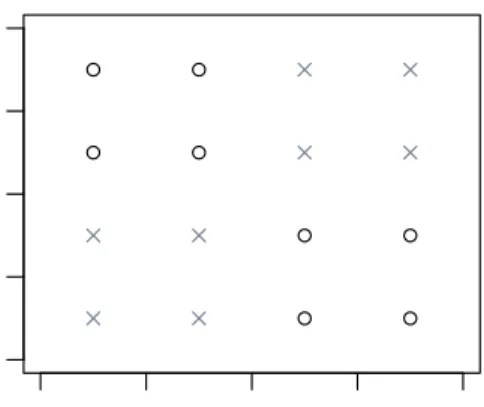
inference trees (seeHothornet al.2006, for references to other algorithms) and avoids selecting variables with many potential splits more often than those with fewer potential splits. 2.3. An illustration of the limitations of locally optimal decision trees A very simple example that illustrates the limitation of forward-search recursive partitioning methods is depicted in Figure1. The example only contains two independent variables and can be solved with three splits that partition the input space into four regions. As expected the recursive partitioning methods rpart and ctree fail to find any split at all, as the loss function on the resulting subsets cannot be reduced by the first split. For methods that explore Θ in a more global fashion it is straightforward to find an optimal solution to this problem. One solution is the tree constructed byevtree:
Model formula: Y ~ X1 + X2
Fitted party: [1] root
● ● ● ● ● ● ● ● 0.0 0.5 1.0 1.5 2.0 0.0 0.5 1.0 1.5 2.0 X1 X2
Figure 1: Class distribution of the (X1, X2)-plane. The two classes are indicated by black circles and gray crosses.
| [2] X2 < 1.25 | | [3] X1 < 1.25: X (n = 4, err = 0.0%) | | [4] X1 >= 1.25: O (n = 4, err = 0.0%) | [5] X2 >= 1.25 | | [6] X1 < 1.25: O (n = 4, err = 0.0%) | | [7] X1 >= 1.25: X (n = 4, err = 0.0%)
Number of inner nodes: 3 Number of terminal nodes: 4
All instances are classified correctly. Each of the terminal nodes 3 and 7 contain four instances of the classX. Four instances of class Oare assigned to each of the terminal nodes 4 and 6.
2.4. Approaches for learning globally optimal decision trees
When compared with the described forward stepwise search, a less greedy approach is to calculate the effects of the split rules deeper down in the tree. In this way optimal trees can be found for simple problems. However, split selection at a given node in Equation 3 has complexityO(P N) (if all P variables are numeric/ordered withN distinct values). Through a global search up toDlevels – i.e., corresponding to a full binary tree withM = 2D terminal nodes – the complexity increases toO(PDND) (Papagelis and Kalles 2001). One conceivable compromise between these two extremes is to look aheadd steps with 1< d < D (see e.g.,
Esmeir and Markovitch 2007), also yielding a locally optimal tree but less constrained than that from a 1-step-ahead search.
Another class of algorithms is given by stochastic optimization methods that, given an initial tree, seek improved solutions through stochastic changes to the tree structure. Thus, these algorithms try to explore the full parameter space Θ but cannot be guaranteed to find the
globally optimal solution but only an approximation thereof. Besides evolutionary algorithms (Koza 1991), Bayesian CART (Denison, Mallick, and Smith 1998) and simulated annealing (Sutton 1991) were used successfully to solve difficult classification and regression tree prob-lems. Koza(1991) first formulated the concept of using evolutionary algorithms as a stochastic optimization method to build classification and regression trees. Papagelis and Kalles(2001) presented a classification tree algorithm and provided results on several datasets from the UCI machine learning repository (Frank and Asuncion 2010). Another method for the con-struction of classification and regression trees via evolutionary algorithms was introduced by
Gray and Fan(2008) andFan and Gray(2005), respectively. Cantu-Paz and Kamath(2003) used an evolutionary algorithm to induce so-called oblique classification trees.
3. The
evtree
algorithm
The general framework of evolutionary algorithms emerged from different representatives.
Holland (1992) called his method genetic algorithms, Rechenberg (1973) invented evolution strategies, andFogel, Owens, and Walsh (1966) introduced evolutionary programming. More recently,Koza (1992) introduced a fourth stream and called itgenetic programming. All four representatives only differ in the technical details, for example the encoding of the individual solutions, but follow the same general outline (Eiben and Smith 2007). Evolutionary algo-rithms are being increasingly widely applied to a variety of optimization and search problems. Common areas of application include data mining (Freitas 2003;Cano, Herrera, and Lozano 2003), statistics (de Mazancourt and Calcagno 2010), signal and image processing (Man, Tang, Kwong, and Halang 1997), and planning and scheduling (Jensen 2003).
The pseudocode for the general evolutionary algorithm is provided in Table1. In the context of classification and regression trees, allindividuals from the population (of some given size) are θs as defined in Equation 1. The details of their evolutionary selection is given below following the general outline displayed in Table1.
As pointed out in Section2, some elementsθ∈Θ are typically excluded in practice to satisfy minimal subsample size requirements. In the following, the terminvalid node refers to such excluded cases, not meeting sample size restrictions.
1. Initialize the population. 2. Evaluate each individual.
3. While(termination condition is not satisfied) do: a. Select parents.
b. Alter selected individuals via variation operators. c. Evaluate new solutions.
d. Select survivors for the next generation.
3.1. Initialization
Each tree of the population is initialized with a valid, randomly generated, split rule in the root node. First,v1 is selected with uniform probability from 1, ..., P. Second, a split point
s1 is selected. If Xv1 is numeric or ordinal with u unique values, a split point s1 is selected with uniform probability from theu−1 possible spit points ofXv1. IfXv1 is nominal and has
ccategories, each k= 1, ..., c has a probability of 50% to be assigned to the left or the right daughter node. In cases where allkare allocated to the same terminal node, the assignment of one category is flipped to the other terminal node. If this procedure results in a non-valid split rule, the two steps of random split variable selection and split point selection are repeated. With the definition ofr= 1 and the selection of v1 and s1, the initialization is complete and each individual of the population of trees is of typeθ1 = (v1, s1).
3.2. Parent selection
In every iteration, each tree is selected once to be modified by one of the variation operators. In cases where the crossover operator is applied, the second parent is selected randomly from the remaining population. In this way, some trees are selected more than once in each iteration.
3.3. Variation operators
Four types of mutation operators and one crossover operator are utilized by our algorithm. In each modification step, one of the variation operators is randomly selected for each tree. The mutation and crossover operators are described below.
Split
Split selects a random terminal-node and assigns a valid, randomly generated, split rule to it. As a consequence, the selected terminal node becomes an internal node r and two new terminal nodes are generated.
The search for a valid split rule is conducted as in see Section3.1 for a maximum ofP iter-ations. In cases where no valid split rule can be assigned to the internal node at position r, the search for a valid split rule is carried out on another randomly selected terminal node. If, after 10 attempts, no valid split rule can be found, thenθi+1 = θi. Otherwise, the set of
parameters in iterationi+ 1 are given byθi+1=θi∪(vr, sr).
Prune
Prune chooses a random internal node r, where r > 1, which has two terminal nodes as successors and prunes it into a terminal node. The tree’s parameters at iteration i+ 1 are
θi+1=θi\(vr, sr). Ifθi only comprises one internal node, i.e., the root node, thenθi+1=θi.
Major split rule mutation
Major split rule mutationselects a random internal node rand changes the split rule, defined by the corresponding split variablevr, and the split point sr. With a probability of 50%, a
value from the range 1, ..., P is assigned tovr. Otherwise vr remains unchanged and onlysr
range of possible values ofXvr is selected, or a non-empty set of categories is assigned to each
of the two terminal nodes. If the split rule at r becomes invalid, the mutation operation is reversed and the procedure, starting with the selection of r, is repeated for a maximum of 3 attempts. Subsequent nodes that become invalid are pruned.
If no pruning occurs, θi and θi+1 contain the same set of parameters. Otherwise, the set of parameters (vm1, sm1, ..., vmf, smf), corresponding to invalid nodes, is removed fromθi. Thus,
θi+1=θi\(vm1, sm1, ..., vmf, smf).
Minor split rule mutation
Minor split rule mutationis similar to themajor split rule mutationoperator, but it does not altervr and only changes the split pointsr by a minor degree. IfXvr is numerical or ordinal
the split pointsris changed by a non-zero number of unique values ofXvr. In cases whereXvr
has less then 20 unique values, the split point is change to to the next larger, or the next lower, unique value ofXvr. Otherwise, sr is randomly shifted by a number of unique values that is
not larger than 10% of the range of unique values ofXvr. If Xvr is a nominal variable, with
less than 20 categories, one of the categories is randomly modified. Otherwise, at least one and at most 10% of the variable’s categories are changed. In cases where subsequent nodes become invalid, further split points are searched that preserve the tree’s topology. After five non-successful attempts at finding a topology preserving split point, the non-valid nodes are pruned.
Equivalently to the major split rule mutation operator the subsequent solution θi+1 = θi \
(vm1, sm1, ..., vmf, smf).
Crossover
Crossoverexchanges, randomly selected, subtrees between two trees. Letθ1
i andθ2i be the two
trees chosen from the population for crossover. First, two internal nodesr1andr2are selected randomly from θ1i and θ2i, respectively. Let sub1(θji, rj) denote the subtree of θj rooted by
rj (j = 1,2), i.e., the tree containing rj and its descendant nodes. Then, the complementary
part of θji can be defined as sub2(θji, rj) =θij\sub1(θji, rj). The crossover operator creates
two new trees θ1i+1 = sub2(θi1, r1)∪sub1(θ2i, r2) and θ2i+1 = sub2(θi2, r2)∪sub1(θi1, r1). If the crossover creates some invalid nods in either one of the new treesθi1+1 or θi2+1, these are omitted.
3.4. Evaluation function
The evaluation function represents the requirements the population should adapt to. In general, these requirements are formulated by Equation 2. A suitable evaluation function for classification and regression trees minimizes the models’ accuracy on the training data, and the models’ complexity. This subsection describes the currently implemented choices of evaluation functions for classification and for regression.
Classification
The quality of a classification tree is most commonly measured as a function of its misclassifi-cation MC and the complexity of a tree by a function of the number of its terminal nodesM.
by logN and a user-specified parameter α, measures the complexity of trees. loss(Y, f(X, θ)) = 2N·MC(Y, f(X, θ)) = 2· N X n=1 I(Yn6=f(X·n, θ)), (5) comp(θ) = α·M·logN.
With these particular choices, Equation 2 seeks trees ˆθ that minimize the misclassification loss at a BIC-type tradeoff with the number of terminal nodes.
Other, existing and commonly used choices of evaluation functions include theBayesian in-formation criterion (BIC, as inGray and Fan 2008) andminimum description length (MDL, as inQuinlan and Rivest 1989). For both evaluation functions deviance is used for accuracy estimation. Deviance is usually preferred over the misclassification rate in recursive partition-ing methods, as it is more sensitive to changes in the node probabilities (Hastie, Tibshirani, and Friedman 2009, pp. 308–310). However, this is not necessarily an advantage for global tree building methods like evolutionary algorithms.
Regression
For regression trees, accuracy is usually measured by the mean squared error MSE. Here, it is again coupled with a BIC-type complexity measure:
UsingN ·log MSE as a loss function and α·4·(M + 1)·logN as the complexity part, the general formulation of the optimization problem in can be rewritten as:
loss(Y, f(X, θ)) = Nlog MSE(Y, f(X, θ)) = Nlog ( N X n=1 (Yn−f(X·n, θ)2) ) , (6) comp(θ) = α·4·(M+ 1)·logN.
Here,M+1 is the effective number of estimated parameters, taking into account the estimates of a mean parameter in each of the terminal nodes and the constant error variance term. With
α= 0.25 the criteria is, up to a constant, equivalent to the BIC used byFan and Gray(2005). However, the effective number of parameters estimated for is actually much higher thanM+1 due to the selection of parameters in the split variable and the selection of the variable itself. It is however unclear how these should be counted (Gray and Fan 2008;Ripley 2008, p. 222). Therefore, a more conservative default value ofα= 1 is assumed.
3.5. Survivor selection
The population size stays constant during the evolution and only a fixed subset of the can-didate solutions can be kept in memory. A common strategy is the (µ+λ) selection, where
µ survivors for the next generation are selected from the union ofµparents andλoffsprings. An alternative approach is the (µ, λ) strategy where µsurvivors for the next generation are selected from λoffsprings.
Our algorithm uses (1 + 1) selection, where one parent solution competes with one offspring for a place in the population. In the case of a mutation operator either the solution beforeθi
or after modificationθi+1 is kept in memory. In the case of the crossover operator, the initial solutions ofθi1 competes with its subsequent solutions θ1i+1. Correspondingly, one of the two solutions θi2 and θi2+1 is rejected. The survivor selection is done deterministically. The tree with lower fitness, according to the evaluation function, is rejected. Note that, due to the definition of the crossover operator, some trees are selected more than once in an iteration. Correspondingly, these trees undergo the survival selection process more than once in an iteration.
As in classification and regression tree analysis the individual solutions are represented by trees. This design offers computational advantages over (µ+λ), with µ >1 and λ >1, and (µ, λ) strategies. In particular, for the application of mutation operators no new trees have to be constructed. The tree after modification is simply accepted or reversed to the previous solution.
There are two important issues in the evolution process of an evolutionary algorithm: popu-lation diversity and selective pressure (Michalewicz 1994). These factors are related, as with increasing selective pressure the search is focused more around the currently best solutions. An overly strong selective pressure can cause the algorithm to converge early in local optima. On the other hand, an overly weak selective pressure can make the search ineffective. Using a (µ+λ) strategy, a strong selective pressure can occur in situations as follows. Suppose the
b-th tree of the population is one of the fittest trees in iterationi, and in iterationione split rule of theb-th tree is changed only by a minor degree. Then very few instances are classified differently and the overall misclassification might not even change. However, as they represent one of the best solutions in iterationi, they are both selected for the subsequent population. This situation can occur frequently, especially when a fine-tuning operator like theminor split rule mutation is used. Then, the diversity of different trees is lost quickly and the algorithm likely terminates in a local optimum. The (1 + 1) selection mechanism clearly avoids these situations, as only the parent or the offspring can be part of the subsequent population.
3.6. Termination
Using the default parameters, the algorithm terminates when the quality of the best 5% of trees stabilizes for 100 iterations, but not before 1000 iterations. If the run does not converge the algorithm terminates after a user-specified number of iterations. In cases where the algorithm does not converge, a warning message is written to the command line. The tree with the highest quality according to the evaluation function is returned.
4. Implementation and application in practice
Packageevtreeprovides an efficient implementation of an evolutionary algorithm that builds classification trees in R. CPU- and memory- intensive tasks are fully computed in C++, while the user interfaces and plot functions are written inR. The.C() interface (Chambers 2008) was used to pass arguments between the two languages. evtree depends on the par-tykitpackage (Hothorn and Zeileis 2011), which provides an infrastructure for representing, summarizing, and visualizing tree-structured models.
4.1. User interface
The principal function of the evtree package is the eponymous function evtree() taking arguments
evtree(formula, data = list(), weights = NULL, subset = NULL, control = evtree.control(...), ...)
where formula, data, weights, and subset specify the data in the usual way, e.g., via
formula = y ~ x1 + x2. Additionally,controlcomprises a list of control parameters
evtree.control(minbucket = 7L, minsplit = 20L, maxdepth = 9L, niterations = 10000L, ntrees = 100L, alpha = 1,
operatorprob = list(pmutatemajor = 0.2, pmutateminor = 0.2, pcrossover = 0.2, psplit = 0.2, pprune = 0.2),
seed = NULL, ...)
where the parametersminbucket,minsplit, andmaxdepthconstrain the solution to a mini-mum number of observations in each terminal node, a minimini-mum number of observation in each internal node and a maximum tree depth. Note that the memory requirements increase by the square of the maximum tree depth. Parameteralpharegulates the complexity parameter
αin Equation5 and6, respectively. niterations andntrees specify the maximum number of iterations and the number of trees in the population, respectively. With the argument
operatorprob, user-specified probabilities for the variation operators can be defined. For making computations reproducible, argumentseedis an optional integer seed for the random number generator (atC++level). If not specified, the random number generator is initialized by as.integer(runif(1, max = 2^16)) in order to inherit the state of .Random.seed (at
Rlevel). If set to-1L, the seed is initializied by the system time.
The trees computed by evtree inherit from class ‘party’ supplied by the partykit pack-age. The methods inherited in this way include standard print(),summary(), and plot()
functions to display trees and a predict() function to compute the fitted response or node number etc.
4.2. Case study: Customer targeting
An interesting application for classification tree analysis is target marketing, where limited resources are aimed at a distinct group of potential customers. An example is provided by
Lilien and Rangaswamy(2004) in theBookbinder’s Book Club marketing case study about a (fictitious) American book club. In this case study, a brochure of the book “The Art History of Florence” was sent to 20,000 customers, 1,806 of which bought the book. The dataset contains a subsample of 1,300 customers for building a predictive model of customer choice. Besides predictive accuracy, model complexity is a crucial issue in this application: Smaller trees are easier to interpret and communicable to marketing experts and management pro-fessionals. Hence, we use evtree with a maximal depth of two levels of splits only. This is contrasted with rpart and ctree with and without such a restriction of tree depth to show that the evolutionary search of the global parameter space can be much more effec-tive in balancing prediceffec-tive accuracy and complexity compared to forward-search recursive partitioning.
All trees are constrained to have a minimum number of 10 observations per terminal node. Additionally, a significance level of 1% is employed in the construction of conditional infer-ence trees which is more appropriate than the default 5% level for 1,300 observations. To provide uniform visualizations and predictions of the fitted models, ‘party’ objects are used to represent all trees. For, ‘rpart’ trees partykit provides a suitable as.party() method while a reimplementation of ctree() is provided in partykit (as opposed to the original in party) that directly leverages the ‘party’ infrastructure.
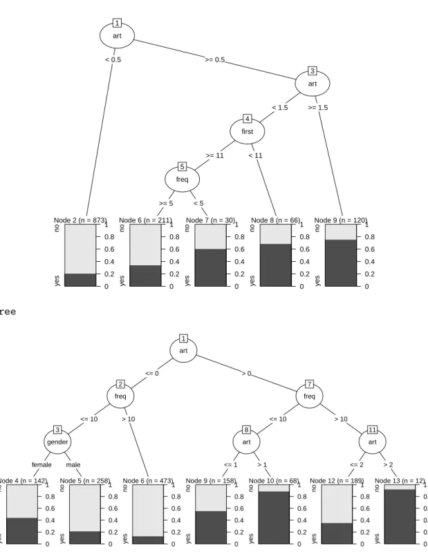
First, the data is loaded and the forward-search trees are grown with and without depth restriction, visualizing the unrestricted trees in Figure2.
R> data("BBBClub", package = "evtree") R> library("rpart")
R> rp <- as.party(rpart(choice ~ ., data = BBBClub, minbucket = 10)) R> rp2 <- as.party(rpart(choice ~ ., data = BBBClub, minbucket = 10,
+ maxdepth = 2))
R> ct <- ctree(choice ~ ., data = BBBClub, minbucket = 10, mincrit = 0.99) R> ct2 <- ctree(choice ~ ., data = BBBClub, minbucket = 10, mincrit = 0.99,
+ maxdepth = 2)
R> plot(rp) R> plot(ct)
With the objective of building a smaller, but at still accurate tree, evtree is constrained to a maximum tree depth of 2, see Figure3.
R> set.seed(1090)
R> ev <- evtree(choice ~ ., data = BBBClub, minbucket = 10, maxdepth = 2)
[1] TRUE
The resulting evolutionary tree is printed below and visualized in Figure3.
R> plot(ev) R> ev
Model formula:
choice ~ gender + amount + freq + last + first + child + youth + cook + diy + art
Fitted party: [1] root
| [2] first < 12
| | [3] art < 1: no (n = 250, err = 30.8%) | | [4] art >= 1: yes (n = 69, err = 30.4%) | [5] first >= 12
| | [6] art < 2: no (n = 864, err = 21.8%) | | [7] art >= 2: yes (n = 117, err = 25.6%)
Number of inner nodes: 3 Number of terminal nodes: 4
rpart art 1 < 0.5 >= 0.5 Node 2 (n = 873) y es no 0 0.2 0.4 0.6 0.8 1 art 3 < 1.5 >= 1.5 first 4 >= 11 < 11 freq 5 >= 5 < 5 Node 6 (n = 211) y es no 0 0.2 0.4 0.6 0.8 1 Node 7 (n = 30) y es no 0 0.2 0.4 0.6 0.8 1 Node 8 (n = 66) y es no 0 0.2 0.4 0.6 0.8 1 Node 9 (n = 120) y es no 0 0.2 0.4 0.6 0.8 1 ctree art 1 <= 0 > 0 freq 2 <= 10 > 10 gender 3 female male Node 4 (n = 142) y es no 0 0.2 0.4 0.6 0.8 1 Node 5 (n = 258) y es no 0 0.2 0.4 0.6 0.8 1 Node 6 (n = 473) y es no 0 0.2 0.4 0.6 0.8 1 freq 7 <= 10 > 10 art 8 <= 1 > 1 Node 9 (n = 158) y es no 0 0.2 0.4 0.6 0.8 1 Node 10 (n = 68) y es no 0 0.2 0.4 0.6 0.8 1 art 11 <= 2 > 2 Node 12 (n = 189) y es no 0 0.2 0.4 0.6 0.8 1 Node 13 (n = 12) y es no 0 0.2 0.4 0.6 0.8 1
Figure 2: Trees for customer targeting constructed byrpart(upper panel) andctree(lower panel). The target variable is the customer’s choice of buying the book. The variables used for splitting are the number of art books purchased previously (art), the number of months since the first purchase (first), the frequency of previous purchases at the Bookbinder’s Book Club (freq) and the customer’sgender.
evtree first 1 < 12 >= 12 art 2 < 1 >= 1 Node 3 (n = 250) y es no 0 0.2 0.4 0.6 0.8 1 Node 4 (n = 69) y es no 0 0.2 0.4 0.6 0.8 1 art 5 < 2 >= 2 Node 6 (n = 864) y es no 0 0.2 0.4 0.6 0.8 1 Node 7 (n = 117) y es no 0 0.2 0.4 0.6 0.8 1
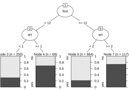
Figure 3: Tree for customer targeting constructed by evtree The target variable is the customer’s choice of buying the book. The variables used for splitting are the number of art books purchased previously (art) and the number of months since the first purchasefirst.
Not surprisingly, the explanatory variableart– the number of art books purchased previously at the book club – plays a key role in all constructed classification trees along with the number of months since the first purchase (first), the frequency of previous purchases (freq) and the customer’s gender. Interestingly, though, the forward-search trees select the arguably most important variable in the first split while the evolutionary tree uses first in the first split andartin both second splits. Thus, the evolutionary tree uses a different cutoff in art
for bookclub members that joined in the last year as opposed to older customers. While the former are predicted to be buyers if they previously bought at least one art book, the latter are predicted to purchase the advertised art book only if they previously bought at least two other art books. Certainly, this classification is easy to understand and communicate (helped by Figure 3) to practitioners.
However, we still need to answer the question how well it performs in contrast to the other trees. Hence, we set up a function mc()the computes the misclassification rate as a measure of predictive accuracy and a functionevalfun() that computes the evaluation function (i.e., penalized by tree complexity) from Equation 5.
R> mc <- function(obj) 1 - mean(predict(obj) == BBBClub$choice) R> evalfun <- function(obj) 2 * nrow(BBBClub) * mc(obj) +
+ width(obj) * log(nrow(BBBClub))
R> trees <- list("evtree" = ev, "rpart" = rp, "ctree" = ct, "rpart2" = rp2, + "ctree2" = ct2)
R> round(sapply(trees, function(obj) c("misclassification" = mc(obj), + "evaluation function" = evalfun(obj))), digits = 3)
evtree rpart ctree rpart2 ctree2 misclassification 0.243 0.238 0.248 0.262 0.255 evaluation function 660.680 655.851 694.191 701.510 692.680
Not surprisingly the evolutionary tree ev outperforms the depth-restricted trees rp2 and
ct2, both in terms of misclassification and the penalized evaluation function. However, it is interesting to see thatevperforms even better than the unrestricted conditional inference tree ct and is comparable in performance to the unrestricted CART tree rp. Hence, the practitioner may choose the evolutionary treeevas it is the easiest to communicate.
Although the constructed trees are considerably different, the code above shows that the pre-dictive accuracy is rather similar. Moreover, below we see that the structure of the individual predictions on the dataset are rather similar as well:
R> ftable(tab <- table(evtree = predict(ev), rpart = predict(rp),
+ ctree = predict(ct), observed = BBBClub$choice))
observed no yes evtree rpart ctree
no no no 799 223 yes 38 24 yes no 0 0 yes 12 18 yes no no 0 0 yes 0 0 yes no 21 19 yes 30 116
R> sapply(c("evtree", "rpart", "ctree"), function(nam) {
+ mt <- margin.table(tab, c(match(nam, names(dimnames(tab))), 4))
+ c(abs = as.vector(rowSums(mt))[2],
+ rel = round(100 * prop.table(mt, 1)[2, 2], digits = 3))
+ })
evtree rpart ctree abs 186.000 216.000 238.000 rel 72.581 70.833 66.387
In this case,evtreeclassifies less customers (186) as buyers asrpart(216) andctree(238). However,evtreeachieves the highest proportion of correct classification among the declared buyers: 72.6% compared to 70.8% (rpart) and 66.4% (ctree).
In summary, this illustrates howevtreecan be employed to better balance predictive accuracy and complexity by searching a larger space of potential trees. As a final note, it is worth pointing out that in this setup, several runs of evtree()with the same parameters typically lead to the same tree. However, this may not always be the case. Due to the stochastic nature of the search algorithm and the vast search space, trees with very different structures but similar evaluation function values may be found by subsequent runs of evtree(). Here, this problem is alleviated by restricting the maximal depth of the tree, yielding a clear solution.
5. Performance comparison
In this section, we compare evtree with rpart and ctree in a more rigorous benchmark comparison.
In the first part of the analysis (Section5.1) the algorithms are compared on 14 benchmark datasets that are publicly available and 3 real-world datasets from the Austrian Diagnosis Related Group (DRG) system (Bundesministerium f¨ur Gesundheit 2010). The analysis is based on the evaluation of 250 bootstrap samples for each of the 20 datasets. The misclassi-fication rate on theout-of-bag (Hothorn, Leisch, Zeileis, and Hornik 2005) samples is used as a measure of predictive accuracy. Furthermore, the complexity is estimated by the number of terminal nodes.
In the second part (Section 5.2) the algorithms’ performances are assessed on an artificial chessboard problem that is simulated with different noise levels. The estimation of predictive accuracy and the number of terminal nodes is based on 250 realizations for each simulation. All models are constrained to a minimum number of 7 observations per terminal node, 20 ob-servations per internal node and a maximum tree depth of 9. Apart from that, the default settings of the algorithms are used. For assessment of significant differences in predictive accu-racy and complexity, respectively, Dunnett’s correction fromRpackage multcomp (Hothorn, Bretz, and Westfall 2008) was used for calculating simultaneous 95% confidence intervals on the individual datasets.
As missing values are currently not supported by evtree (e.g., by surrogate splits), the 16 missing values in the Breast Cancer Database – the only dataset in the study with missing values – were removed before analysis.
5.1. Benchmark and real-world problems
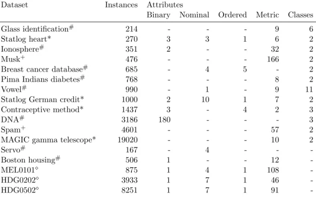
In Table 2 the benchmark and real-world datasets from the Austrian DRG system are de-scribed. In the Austrian DRG system, resources are allocated to hospitals by simple rules mainly regarding the patients’ diagnoses, procedures, and age. Regression tree analysis is performed to model patient groups with similar resource consumption. A more detailed de-scription of the datasets and the application can be found in Grubinger, Kobel, and Pfeiffer
(2010).
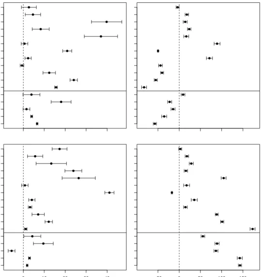
The relative performance of evtree and rpart is summarized in Figure 4 (upper panels). Performance differences are displayed relative to evtree’s performance. For example, on the Glass dataset, the average misclassification rate ofrpartis 2.7% higher than the misclassifi-cation rate of evtree. It can be observed that on 12 out of 17 datasetsevtree significantly outperformsrpartin terms of predictive accuracy. Only on theContraceptive Methoddataset
evtree performs slightly worse. In terms of complexity,evtreemodels are significantly more complex on 10 and less complex on 7 datasets.
Figure4(lower panels) summarizes the relative performance ofevtreeandctree. For 15 out of 17 datasetsevtree shows a better predictive performance. The algorithms’ performances is significantly worse on the MEL0101 dataset, where the average misclassifiation rate of
ctree is 5.6% lower. However, on this dataset, ctree models are on average 86.5% larger thanevtree models. The relative complexity ofevtreemodels is significantly smaller for 15 and larger for 1 dataset.
Dataset Instances Attributes
Binary Nominal Ordered Metric Classes
Glass identification# 214 - - - 9 6
Statlog heart* 270 3 3 1 6 2
Ionosphere# 351 2 - - 32 2
Musk+ 476 - - - 166 2
Breast cancer database# 685 - 4 5 - 2
Pima Indians diabetes# 768 - - - 8 2
Vowel# 990 - 1 - 9 11
Statlog German credit* 1000 2 10 1 7 2
Contraceptive method* 1437 3 - 4 2 3
DNA# 3186 180 - - - 3
Spam+ 4601 - - - 57 2
MAGIC gamma telescope* 19020 - - - 10 2
Servo# 167 - 4 - -
-Boston housing# 506 1 - - 12
-MEL0101 875 1 4 1 108
-HDG0202 3933 1 7 1 46
-HDG0502 8251 1 7 1 91
-Table 2: Description of the evaluated benchmark datasets. The datasets marked with ∗ originate from the UCI machine learning repository (Frank and Asuncion 2010) and are made available in the evtree package. Datasets marked with # and + are from the R packages mlbench (Leisch and Dimitriadou 2010) and kernlab (Karatzoglou et al. 2004), respectively. The three real-world datasets from the Austrian DRG system are marked with.
While the smallest of the analyzed datasets, Glass identification, only needed approximately 4–6 seconds to fit, larger datasets demanded several minutes. The fit of a model from the largest dataset,MAGIC gamma telescope, required approximately 40–50 minutes and a main memory of 400 Mbit. The required resources were measured on an Intel Core 2 Duo with 2.2 GHz and 2 GB RAM using the 64-bit version of Ubuntu 10.10.
Another important issue to be considered is the random nature of evolutionary algorithms. For larger datasets, frequently, considerable different solutions exist that yield a similar or even the same evaluation function value. Therefore, subsequent runs of evtree can result in very different tree structures. This is not a problem if the tree is intended only for predictive purposes, and it is also not a big issue for many decision and prognosis tasks. Typically, in such applications, the resulting model has to be accurate, compact, and meaningful in its interpretation, but the particular tree structure is of secondary importance. Examples of such applications include the presented marketing case study and the Austrian DRG system. In cases where a model is not meaningful in its interpretation, the possibility of constructing different trees can even be beneficial. However, if the primary goal is to interpret relationships in the data, based on the selected splits, the random nature of the algorithm has to be considered.
● ● ● ● ● ● ● ● ● ● ● ● ● ● ● ● ● HDG0502 HDG0202 MEL0101 Boston housing Servo Magic gamma telescope Spam DNA Contraceptive method Statlog German credit Vowel Pima Indians diabetes Breast cancer database Musk Ionosphere Statlog heart Glass identification rpart ● ● ● ● ● ● ● ● ● ● ● ● ● ● ● ● ● ● ● ● ● ● ● ● ● ● ● ● ● ● ● ● ● ● 0 10 20 30 40 HDG0502 HDG0202 MEL0101 Boston housing Servo Magic gamma telescope Spam DNA Contraceptive method Statlog German credit Vowel Pima Indians diabetes Breast cancer database Musk Ionosphere Statlog heart Glass identification
ctree
relative difference in predictive accuracy (%)
● ● ● ● ● ● ● ● ● ● ● ● ● ● ● ● ● −50 0 50 100 150 relative difference in complexity (%)
Figure 4: Performance comparison ofevtreevs.rpart(upper panels) andevtreevs.ctree
(lower panels). Prediction error (left panels) is compared by the relative difference of the misclassification rate or the mean-squared error. The complexity (right panels) is compared by the relative difference of the number of terminal nodes.
5.2. Artificial problem
In this section we demonstrate the ability of evtree to solve an artificial problem that is difficult to solve for most recursive classification tree algorithms (Loh 2009). The data was simulated with 2000 instances for both the training-set and the test-set. Predictor variables
X1 and X2 are simulated to be uniformly distributed in the interval [0,4]. The classes are distributed in alternating squares forming a 4×4 chessboard in the (X1, X2)-plane. One realization of the simulated data is shown in Figure5. Furthermore, variables X3 −X8 are
● ● ● ● ● ● ● ● ● ● ● ● ● ● ● ● ● ● ● ● ● ● ● ● ● ● ● ● ● ● ● ● ● ● ● ● ● ● ● ● ● ● ● ● ● ● ● ● ● ● ● ● ● ● ● ● ● ● ● ● ● ● ● ● ● ● ● ● ● ● ● ● ● ● ● ● ● ● ● ● ● ● ● ● ● ● ● ● ● ● ● ● ● ● ● ● ● ● ● ● ● ● ● ● ● ● ● ● ● ● ● ● ● ● ● ● ● ● ● ● ● ● ● ● ● ● ●● ● ● ● ● ● ● ● ● ● ● ● ● ● ● ● ● ● ● ● ● ● ● ● ●● ● ● ● ● ● ● ● ● ● ● ● ● ● ● ● ● ● ● ● ● ● ● ● ● ● ● ● ● ● ● ● ● ● ● ● ● ● ● ● ● ● ● ● ● ● ● ● ● ● ● ● ● ● ● ● ● ● ● ● ● ● ● ● ● ● ● ● ● ● ● ● ● ● ● ● ● ● ● ● ● ● ● ● ● ● ● ● ● ● ● ● ● ● ● ● ● ● ● ● ● ● ● ● ● ● ● ● ● ● ● ● ● ● ● ● ● ● ● ● ● ● ● ● ● ● ● ● ● ● ● ● ● ● ● ● ● ● ● ● ● ● ● ● ● ● ● ● ● ● ● ● ● ● ● ● ● ● ● ● ● ● ● ● ● ● ● ● ● ● ● ● ● ● ● ●●● ● ● ● ● ● ● ● ● ● ● ● ● ● ● ● ● ● ● ● ● ● ● ● ● ● ● ● ● ● ● ● ● ● ● ● ● ● ● ● ● ● ● ● ● ● ● ● ● ● ● ● ● ● ● ● ● ● ● ● ● ● ● ● ● ● ● ● ● ● ● ● ● ● ● ● ● ● ● ● ● ● ● ● ● ● ● ● ● ● ● ● ● ● ● ● ● ● ● ● ●● ● ● ● ● ● ● ● ● ● ● ● ● ● ● ● ● ● ● ● ● ● ● ● ● ● ● ● ● ● ● ● ● ● ● ● ● ● ● ● ● ● ● ● ● ● ● ● ● ● ● ● ● ● ● ● ● ● ● ● ● ● ● ● ● ●● ● ● ● ● ● ● ● ● ● ● ● ● ● ● ● ● ● ● ● ● ● ● ● ● ● ● ● ● ● ● ● ● ● ● ● ● ● ● ● ● ● ● ● ● ● ● ● ● ● ● ● ● ● ● ● ● ● ● ● ● ● ● ● ● ● ● ● ● ● ● ● ● ● ● ● ● ● ● ● ● ● ● ● ● ● ● ● ● ●● ● ● ● ● ● ● ● ● ● ● ● ● ● ● ● ● ● ● ● ● ● ● ● ● ● ● ● ● ● ● ● ● ● ● ● ● ● ● ● ●● ●● ● ● ● ● ● ● ● ● ● ● ● ● ● ● ● ● ● ● ● ● ● ● ● ● ● ● ● ● ● ● ● ● ● ● ● ● ● ● ● ● ● ● ● ● ● ● ● ● ● ● ● ● ● ● ● ● ● ● ● ● ● ● ● ● ● ● ● ● ● ● ● ● ● ● ● ● ● ● ● ● ● ● ● ● ● ● ● ● ● ● ● ● ● ● ● ● ● ● ● ● ● ● ● ● ● ● ● ● ● ● ● ● ● ● ● ● ● ● ●● ● ● ● ● ● ● ● ● ● ● ● ● ● ● ● ● ● ● ● ● ● ● ● ● ● ● ● ● ● ● ● ● ● ● ● ● ● ● ● ● ● ● ● ● ● ● ● ● ● ● ● ● ● ● ● ● ● ● ● ● ● ● ● ● ● ● ● ● ● ● ● ● ● ● ● ● ● ● ● ● ● ● ● ● ● ● ● ● ● ● ● ● ● ● ● ● ● ● ● ● ● ● ● ● ● ● ● ● ● ● ● ● ● ● ● ● ● ● ● ● ● ● ● ● ● ● ● ● ● ● ● ● ● ● ● ● ● ● ● ● ● ● ● ● ● ● ● ● ● ● ● ● ● ● ● ● ● ● ● ● ● ● ● ● ● ● ● ● ● ● ● ● ● ● ● ● ● ● ● ● ● ● ● ● ● ● ● ● ● ● ● ● ● ● ● ● ● ● ● ● ● ● ● ● ● ● ● ● ● ● ● ● ● ● ● ● ● ● ● ● ● ● ● ● ● ● ● ● ●● ● ● ● ● ● ● ● ● ● ● ● ● ● ● ● ● ● ● ● ● ● ● ● ● ● ● ● ● ● ● ● ● ● ● ● ● ● ● ● ● ● ● ● ● ● ● ● ● ● ● ● ● ● ● ● ● ● ● ● ● ● ● ● ● ● ● ● ● ● ● ● ● ● ● 0 1 2 3 4 0 1 2 3 4 X1 X2
Figure 5: Class distribution of the simulated 4×4 chessboard problem with zero noise, plotted on the (X1, X2)-plane. The two classes are indicated by black circles and gray crosses, respectively.
noise variables that are uniformly distributed on the interval [0, 1]. The ideal model for this problem only uses variables X1 and X2 and has 16 terminal nodes, whereas each terminal node comprises the observations that are in the region of one square. Two further simulations are done in the same way, but 5% and 10% percent of the class labels are randomly changed to the other class.
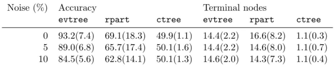
The results are summarized in Table 3. It can be seen that, in the absence of noise, rpart
models on average classify 69.1% of the data points correctly and had 16.6 terminal nodes. An average ctreemodel only has 1.1 terminal nodes and a classification accuracy of 49.9%. In contrast,evtree classifies 93.2% of the instances correctly and requires 14.4 terminal nodes. In the presence of 5% and 10% noise, evtreeclassifies 89.0% and 84.5% of the data correctly.
Noise (%) Accuracy Terminal nodes
evtree rpart ctree evtree rpart ctree
0 93.2(7.4) 69.1(18.3) 49.9(1.1) 14.4(2.2) 16.6(8.2) 1.1(0.3) 5 89.0(6.8) 65.7(17.4) 50.1(1.6) 14.4(2.2) 14.6(8.0) 1.1(0.7) 10 84.5(5.6) 62.8(14.1) 50.1(1.3) 14.6(2.0) 14.3(7.3) 1.1(0.4)
Table 3: Mean (and standard deviation) of accuracy and number of terminal nodes for simu-lated 4×4 chessboard examples.
6. Conclusions
trees that are grown by an evolutionary algorithm. The package uses standard print(),
summary(), and plot() functions to display trees and a predict() function to predict the class labels of new data from the partykit package. As evolutionary learning of trees is computationally demanding, most calculations are conducted in C++. At the moment our algorithm does not support parallelism. However, we intend to extend evtree to parallel computing.
The comparisons with recursive partitioning methodsrpart and ctree in Sections 4 and 5
shows thatevtreeperforms very well in a wide variety of settings, often balancing predictive accuracy and complexity better than the forward-search methods.
However, the goal ofevtree is not to replace the well-established algorithms likerpart and
ctree but rather to complement the tree toolbox with an alternative method which may perform better given sufficient amounts of time and main memory. By the nature of the algorithm it is able to discover patterns which cannot be modeled by a greedy forward-search algorithm. As evtree models can be substantially different to recursively fitted models, it can be beneficial to use both approaches, as this may reveal additional relationships in the data.
References
B¨ack T (1996). Evolutionary Algorithms in Theory and Practice. Oxford University Press, New York.
Breiman L, Friedman JH, Olshen RA, Stone CJ (1984). Classification and Regression Trees. Wadsworth, Belmont.
Bundesministerium f¨ur Gesundheit (2010). “The Austrian DRG System.” URL: http: //www.bmg.gv.at/home/EN/Topics/The_Austrian_DRG_system_brochure_ (accessed on 2011-09-27).
Cano JR, Herrera F, Lozano M (2003). “Using Evolutionary Algorithms as Instance Selection for Data Reduction in KDD: An Experimental Study.”IEEE Transactions on Evolutionary Computation,7(6), 561–575.
Cantu-Paz E, Kamath C (2003). “Inducing Oblique Decision Trees with Evolutionary Algo-rithms.”IEEE Transactions on Evolutionary Computation,7(1), 54–68.
Chambers JM (2008). Software for Data Analysis: Programming with R. Springer-Verlag, New York.
de Mazancourt C, Calcagno V (2010). “glmulti: An R Package for Easy Automated Model Selection with (Generalized) Linear Models.”Journal of Statistical Software,34(12), 1–29. URLhttp://www.jstatsoft.org/v34/i12/.
Denison DGT, Mallick BK, Smith AFM (1998). “A Bayesian CART Algorithm.”Biometrika,
85(2), 363–377.
Eiben AE, Smith JE (2007). Introduction to Evolutionary Computing. Springer-Verlag, New York.
Esmeir S, Markovitch S (2007). “Anytime Learning of Decision Trees.” Journal of Machine Learning Research,8, 891–933.
Fan G, Gray JB (2005). “Regression Tree Analysis Using TARGET.” Journal of Computa-tional and Graphical Statistics,14(1), 206–218.
Fogel LJ, Owens AJ, Walsh MJ (1966). Artificial Intelligence Through Simulated Evolution. John Wiley & Sons, New York.
Frank A, Asuncion A (2010). “UCI Machine Learning Repository.” URLhttp://archive. ics.uci.edu/ml/.
Freitas AA (2003). “A Survey of Evolutionary Algorithms for Data Mining and Knowledge Discovery.” pp. 819–845. Springer-Verlag, New York.
Gray JB, Fan G (2008). “Classification Tree Analysis Using TARGET.” Computational Statistics & Data Analysis,52(3), 1362–1372.
Grubinger T, Kobel C, Pfeiffer KP (2010). “Regression Tree Construction by Bootstrap: Model Search for DRG-Systems Applied to Austrian Health-Data.” BMC Medical Infor-matics and Decision Making,10(9). doi:10.1186/1472-6947-10-9.
Hastie T, Tibshirani R, Friedman J (2009). The Elements of Statistical Learning: Data Mining, Inference, and Prediction. 2nd edition. Springer-Verlag, New York.
Holland JH (1992). Adaptation in Natural and Artificial Systems: An Introductory Analysis with Applications to Biology, Control, and Artificial Intelligence. MIT Press, Cambridge. Hornik K, Buchta C, Zeileis A (2009). “Open-Source Machine Learning: R Meets Weka.”
Computational Statistics,24(2), 225–232.
Hothorn T (2011). “CRAN Task View: Machine Learning.” Version 2011-05-20, URLhttp: //CRAN.R-project.org/view=MachineLearning.
Hothorn T, Bretz F, Westfall P (2008). “Simultaneous Inference in General Parametric Mod-els.”Biometrical Journal,50(3), 346–363.
Hothorn T, Hornik K, Zeileis A (2006). “Unbiased Recursive Partitioning: A Conditional Inference Framework.”Journal of Computational and Graphical Statistics,15(3), 651–674.
Hothorn T, Leisch F, Zeileis A, Hornik K (2005). “The Design and Analysis of Benchmark Experiments.”Journal of Computational and Graphical Statistics,14(3), 675–699.
Hothorn T, Zeileis A (2011). “partykit: A Toolkit for Recursive Partytioning.” R package version 0.1-1, URLhttp://CRAN.R-project.org/package=partykit.
Hyafil L, Rivest RL (1976). “Constructing Optimal Binary Decision Trees Is NP-Complete.” Information Processing Letters,5(1), 15–17.
Jensen MT (2003). “Generating Robust and Flexible Job Shop Schedules Using Genetic Algorithms.”IEEE Transactions on Evolutionary Computation,7(3), 275–288.
Karatzoglou A, Smola A, Hornik K, Zeileis A (2004). “kernlab – An S4 Package for Kernel Methods inR.”Journal of Statistical Software,11(9), 1–20. URLhttp://www.jstatsoft. org/v11/i09/.
Kooperberg C, Ruczinski I (2011). LogicReg: Logic Regression. R package version 1.4.10, URLhttp://CRAN.R-project.org/package=LogicReg.
Koza JR (1991). “Concept Formation and Decision Tree Induction Using the Genetic Pro-gramming Paradigm.” InProceedings of the 1st Workshop on Parallel Problem Solving from Nature, pp. 124–128. Springer-Verlag, London.
Koza JR (1992). Genetic Programming: On the Programming of Computers by Means of Natural Selection. MIT Press, Cambridge, MA.
Leisch F, Dimitriadou E (2010). mlbench: Machine Learning Benchmark Problems. R pack-age version 2.1-0, URLhttp://CRAN.R-project.org/package=mlbench.
Lilien GL, Rangaswamy A (2004). Marketing Engineering: Computer-Assisted Marketing Analysis and Planning. 2nd edition. Trafford Publishing, Victoria, BC.
Loh WY (2009). “Improving the Precision of Classification Trees.”Annals of Applied Statistics,
3(4), 1710–1737.
Man KF, Tang KS, Kwong S, Halang WA (1997). Genetic Algorithms for Control and Signal Processing. Springer-Verlag, New York.
Michalewicz Z (1994). Genetic Algorithms Plus Data Structures Equals Evolution Programs. Springer-Verlag, New York.
Murthy SK, Salzberg S (1995). “Decision Tree Induction: How Effective Is the Greedy Heuris-tic?” In UM Fayyad, R Uthurusamy (eds.),Proceedings of the First International Confer-ence on Knowledge Discovery and Data Mining, pp. 222–227. AAAI Press, San Mateo. Papagelis A, Kalles D (2001). “Breeding Decision Trees Using Evolutionary Techniques.” In
CE Brodley, AP Danyluk (eds.),Proceedings of the Eighteenth International Conference on Machine Learning, pp. 393–400. Morgan Kaufmann Publishers, San Mateo.
Quinlan JR (1992). “Learning with Continuous Classes.” InProceedings of the 5th Australian Joint Conference on Artificial Intelligence, pp. 343–348. World Scientific.
Quinlan JR (1993). C4.5: Programs for Machine Learning. Morgan Kaufmann Publishers, San Mateo.
Quinlan JR, Rivest RL (1989). “Inferring Decision Trees Using the Minimum Description Length Principle.”Information and Computation,80(3), 227–248.
RDevelopment Core Team (2011).R: A Language and Environment for Statistical Computing.
RFoundation for Statistical Computing, Vienna, Austria. ISBN 3-900051-07-0, URLhttp: //www.R-project.org/.
Rechenberg I (1973). Evolutionsstrategie: Optimierung Technischer Systeme nach Prinzipien der Biologischen Evolution. Frommann-Holzboog Verlag, Stuttgart.
Ripley BD (2008). Pattern Recognition and Neural Networks. Cambridge University Press, Cambridge.
Sutton CD (1991). “Improving Classification Trees with Simulated Annealing.” In EM Kerami-das, SM Kaufman (eds.),Computing Science and Statistics: Proceedings of the 23rd Sympo-sium on the Interface, pp. 333–344. Interface Foundation of North America, Fairfax Station. Therneau TM, Atkinson EJ (1997). “An Introduction to Recursive Partitioning Using the
rpartRoutines.”Technical Report 61. URLhttp://www.mayo.edu/hsr/techrpt/61.pdf. Witten IH, Frank E (2011). Data Mining: Practical Machine Learning Tools and Techniques.
3rd edition. Morgan Kaufmann Publishers, San Francisco.
Zantema H (2000). “Finding Small Equivalent Decision Trees Is Hard.”International Journal of Foundations of Computer Science,11(2), 343–354.
Zeileis A, Hothorn T, Hornik K (2008). “Model-Based Recursive Partitioning.” Journal of Computational and Graphical Statistics,17(2), 492–514.
Affiliation:
Thomas Grubinger, Karl-Peter Pfeiffer Innsbruck Medical University
Department for Medical Statistics, Informatics and Health Economics 6020, Innsbruck, Austria
E-mail: [email protected],[email protected] URL:http://www.i-med.ac.at/msig/mitarbeiter/grubinger/ http://www.i-med.ac.at/msig/mitarbeiter/pfeiffer/ Achim Zeileis Universit¨at Innsbruck Department of Statistics 6020, Innsbruck, Austria E-mail: [email protected] URL:http://eeecon.uibk.ac.at/~zeileis/
http://eeecon.uibk.ac.at/wopec/
2011-20 Thomas Grubinger, Achim Zeileis, Karl-Peter Pfeiffer: evtree: Evolu-tionary learning of globally optimal classification and regression trees in R
2011-19 Wolfgang Rinnergschwentner, Gottfried Tappeiner, Janette Walde:
Multivariate stochastic volatility via wishart processes - A continuation
2011-18 Jan Verbesselt, Achim Zeileis, Martin Herold: Near Real-Time Distur-bance Detection in Terrestrial Ecosystems Using Satellite Image Time Series: Drought Detection in Somalia
2011-17 Stefan Borsky, Andrea Leiter, Michael Pfaffermayr: Does going green pay off? The effect of an international environmental agreement on tropical timber trade
2011-16 Pavlo Blavatskyy: Stronger Utility
2011-15 Anita Gantner, Wolfgang H¨ochtl, Rupert Sausgruber:The pivotal me-chanism revisited: Some evidence on group manipulation
2011-14 David J. Cooper, Matthias Sutter: Role selection and team performance
2011-13 Wolfgang H¨ochtl, Rupert Sausgruber, Jean-Robert Tyran:Inequality aversion and voting on redistribution
2011-12 Thomas Windberger, Achim Zeileis: Structural breaks in inflation dyna-mics within the European Monetary Union
2011-11 Loukas Balafoutas, Adrian Beck, Rudolf Kerschbamer, Matthias Sutter: What drives taxi drivers? A field experiment on fraud in a market for credence goods
2011-10 Stefan Borsky, Paul A. Raschky: A spatial econometric analysis of com-pliance with an international environmental agreement on open access re-sources
2011-09 Edgar C. Merkle, Achim Zeileis: Generalized measurement invariance tests with application to factor analysis
2011-08 Michael Kirchler, J¨urgen Huber, Thomas St¨ockl: Thar she bursts -reducing confusion reduces bubbles modified version forthcoming in
2011-06 Octavio Fern´andez-Amador, Martin G¨achter, Martin Larch, Georg Peter: Monetary policy and its impact on stock market liquidity: Evidence from the euro zone
2011-05 Martin G¨achter, Peter Schwazer, Engelbert Theurl: Entry and exit of physicians in a two-tiered public/private health care system
2011-04 Loukas Balafoutas, Rudolf Kerschbamer, Matthias Sutter: Distribu-tional preferences and competitive behavior forthcoming in
Journal of Economic Behavior and Organization
2011-03 Francesco Feri, Alessandro Innocenti, Paolo Pin:Psychological pressure in competitive environments: Evidence from a randomized natural experiment: Comment
2011-02 Christian Kleiber, Achim Zeileis: Reproducible Econometric Simulations
2011-01 Carolin Strobl, Julia Kopf, Achim Zeileis: A new method for detecting differential item functioning in the Rasch model
2010-29 Matthias Sutter, Martin G. Kocher, Daniela R¨utzler and Stefan T. Trautmann: Impatience and uncertainty: Experimental decisions predict adolescents’ field behavior
2010-28 Peter Martinsson, Katarina Nordblom, Daniela R¨utzler and Matt-hias Sutter: Social preferences during childhood and the role of gender and age - An experiment in Austria and Sweden Revised version forthcoming in Economics Letters
2010-27 Francesco Feri and Anita Gantner: Baragining or searching for a better price? - An experimental study. Revised version accepted for publication in Games and Economic Behavior
2010-26 Loukas Balafoutas, Martin G. Kocher, Louis Putterman and Matt-hias Sutter: Equality, equity and incentives: An experiment
2010-25 Jes´us Crespo-Cuaresma and Octavio Fern´andez Amador: Business cycle convergence in EMU: A second look at the second moment
2010-24 Lorenz Goette, David Huffman, Stephan Meier and Matthias Sutter:
Group membership, competition and altruistic versus antisocial punishment: Evidence from randomly assigned army groups
2010-23 Martin G¨achter and Engelbert Theurl:Health status convergence at the local level: Empirical evidence from Austria (revised Version March 2011)
2010-21 Octavio Fern´andez-Amador, Josef Baumgartner and Jes´us Crespo-Cuaresma: Milking the prices: The role of asymmetries in the price trans-mission mechanism for milk products in Austria
2010-20 Fredrik Carlsson, Haoran He, Peter Martinsson, Ping Qin and Matt-hias Sutter: Household decision making in rural China: Using experiments to estimate the influences of spouses
2010-19 Wolfgang Brunauer, Stefan Lang and Nikolaus Umlauf:Modeling hou-se prices using multilevel structured additive regression
2010-18 Martin G¨achter and Engelbert Theurl:Socioeconomic environment and mortality: A two-level decomposition by sex and cause of death
2010-17 Boris Maciejovsky, Matthias Sutter, David V. Budescu and Patrick Bernau: Teams make you smarter: Learning and knowledge transfer in auc-tions and markets by teams and individuals
2010-16 Martin G¨achter, Peter Schwazer and Engelbert Theurl: Stronger sex but earlier death: A multi-level socioeconomic analysis of gender differences in mortality in Austria
2010-15 Simon Czermak, Francesco Feri, Daniela R¨utzler and Matthias Sut-ter:Strategic sophistication of adolescents - Evidence from experimental normal-form games
2010-14 Matthias Sutter and Daniela R¨utzler: Gender differences in competition emerge early in live
2010-13 Matthias Sutter, Francesco Feri, Martin G. Kocher, Peter Martins-son, Katarina Nordblom and Daniela R¨utzler: Social preferences in childhood and adolescence - A large-scale experiment
2010-12 Loukas Balafoutas and Matthias Sutter: Gender, competition and the efficiency of policy interventions
2010-11 Alexander Strasak, Nikolaus Umlauf, Ruth Pfeifer and Stefan Lang:
Comparing penalized splines and fractional polynomials for flexible modeling of the effects of continuous predictor variables
2010-10 Wolfgang A. Brunauer, Sebastian Keiler and Stefan Lang: Trading strategies and trading profits in experimental asset markets with cumulative information
2010-09 Thomas St¨ockl and Michael Kirchler: Trading strategies and trading profits in experimental asset markets with cumulative information
experiment: Comment
2010-07 Michael Hanke and Michael Kirchler: Football Championships and Jer-sey sponsors’ stock prices: An empirical investigation
2010-06 Adrian Beck, Rudolf Kerschbamer, Jianying Qiu and Matthias Sut-ter: Guilt from promisebreaking and trust in markets for expert services -Theory and experiment
2010-05 Martin G¨achter, David A. Savage and Benno Torgler: Retaining the thin blue line: What shapes workers’ intentions not to quit the current work environment
2010-04 Martin G¨achter, David A. Savage and Benno Torgler:The relationship between stress, strain and social capital
2010-03 Paul A. Raschky, Reimund Schwarze, Manijeh Schwindt and Fer-dinand Zahn: Uncertainty of governmental relief and the crowding out of insurance
2010-02 Matthias Sutter, Simon Czermak and Francesco Feri: Strategic sophi-stication of individuals and teams in experimental normal-form games
2010-01 Stefan Lang and Nikolaus Umlauf: Applications of multilevel structured additive regression models to insurance data
Working Papers in Economics and Statistics
2011-20
Thomas Grubinger, Achim Zeileis, Karl-Peter Pfeiffer
evtree: Evolutionary learning of globally optimal classification and regression trees in R
Abstract
Commonly used classification and regression tree methods like the CART algorithm are recursive partitioning methods that build the model in a forward stepwise search. Although this approach is known to be an efficient heuristic, the results of recursive tree methods are only locally optimal, as splits are chosen to maximize homogeneity at the next step only. An alternative way to search over the parameter space of trees is to use global optimization methods like evolutionary algorithms. This pa-per describes the evtree package, which implements an evolutionary algorithm for learning globally optimal classification and regression trees in R. Computationally intensive tasks are fully computed in C++ while the partykit (Hothorn and Zeileis 2011) package is leveraged for representing the resulting trees in R, providing unified infrastructure for summaries, visualizations, and predictions. evtree is compared to rpart (Therneau and Atkinson 1997), the open-source CART implementation, and conditional inference trees (ctree, Hothorn, Hornik, and Zeileis 2006). The usefulness of evtree is illustrated in a textbook customer classification task and a benchmark study of predictive accuracy in which evtree achieved at least similar and most of the time better results compared to the recursive algorithms rpart and ctree.
ISSN 1993-4378 (Print) ISSN 1993-6885 (Online)