Predictive modelling of SAP ERP Applications: Challenges and Solutions

Predictive modelling of SAP ERP Applications: Challenges

and Solutions

: Automated Infrastructure Lab, HP Labs, Bristol, UK, e-mail: [email protected] 2

: SAP Research, CEC Belfast, UK, e-mail: [email protected] 3

: University of Calgary,Calgary, AB, Canada, e-mail: [email protected]

ABSTRACT

Analytic performance models are being increasingly used to support system runtime optimization. This paper consid-ers the modelling features needed to predict the response time behaviour of an industrial enterprise resource plan-ning (ERP) application, SAP ERP. A number of studies have reported modelling success with the application of basic product-form Queueing Network Models (QNMs) to multi-tier systems. Such QNMs are often preferred in the context of optimization studies due to the low computational costs of their solution. However, we show that these simple models do not support many important features required to accu-rately characterize industrial applications such as ERP sys-tems. Specifically, our results indicate that software thread-ing levels, asynchronous database calls, priority schedulthread-ing, multiple phases of processing, and the parallelism offered by multi-core processors all have a significant impact on re-sponse time that cannot be neglected.

Starting from these observations, the paper shows that Layered Queueing Models (LQMs) are a robust alternative to basic QNMs, while still enjoying analytical solution algo-rithms that facilitate their integration in optimization stud-ies. A case study for a sales and distribution workload demonstrates that many of the features supported by LQMs are critical for achieving good prediction accuracy. Results show that, remarkably,all of the featureswe considered that are not captured by basic product-form QNMs are needed to predict mean response times to within 15% of measured values for a wide range of load levels. If any key feature is absent, the mean response time estimates could differ by 36% to 117% compared to the measured values, thus making the case that such non-product-form modelling features are needed for complex real-world applications.

1.

INTRODUCTION

Analytic performance models have traditionally been used to support sizing and capacity planning for computer sys-tems and applications. As the enterprise computing

environ-Permission to make digital or hard copies of all or part of this work for personal or classroom use is granted without fee provided that copies are not made or distributed for profit or commercial advantage and that copies bear this notice and the full citation on the first page. To copy otherwise, or republish, to post on servers or to redistribute to lists, requires prior specific permission and/or a fee.

ROSSA 2009, October 19, 2009 - Pisa, Italy.

Copyright 2009 ICST 978-963-9799-70-7/00/0004 $5.00.

ments evolve towards adaptive and on-demand Infrastruc-ture as a Service (IaaS) paradigms, such models may also be used to support runtime optimization [2]. In particular, models can be exploited to tune the use of resources and guide the acquisition and release of resources. This paper considers the use of analytic models in support of runtime optimization for a complex enterprise application environ-ment. In particular, we focus on the performance analysis of the SAP Enterprise Resource Planning (SAP ERP, for-merly SAP R/3) application [26].

SAP ERP is an integrated backend application with tens of thousands of installations worldwide designed for track-ing and managtrack-ing business processes in midsize and large enterprises. From a technical perspective, this application is built on top of a software integration platform that pro-vides primitives to control the concurrency offered by appli-cation server and database server, the layered use of servers, asynchronous messaging, and priority scheduling for certain types of processing.

Different predictive techniques can be used to support runtime optimization for enterprise systems. Machine learn-ing, analytic, and simulation modelling approaches are the most common [13, 32, 15]. Machine learning techniques fit models to observed data but are not able to anticipate per-formance when either the system infrastructure or the appli-cation undergo significant changes that have not been pre-viously observed. Product-form Queueing Network Models (QNMs) are analytic stochastic models with efficient solu-tion techniques, e.g., Mean Value Analysis (MVA) [17], that can be exploited for runtime optimization and performance prediction. However, they can be difficult to apply because system behavior does not typically satisfy the assumptions needed to enable the efficient solutions for such models, e.g., assumptions on scheduling and service time distributions [3]. To overcome these limitations, analytic models often include heuristics that must be validated, as is the case for the Lay-ered Queueing Model (LQM) paradigm [24, 11] explored in this paper. In general, simulation models can do whatever analytic models can do, but require significantly more time to provide results with sufficiently tight confidence intervals. Even simulations that last several seconds can be too expen-sive to use in an optimization program that evaluates hun-dreds or thousands of models before returning the optimal solution. For this reason, an analytic model is preferable to a simulation model when it offers consistently accurate predictions.

This paper investigates the accuracy of various analytic modelling approaches for the SAP ERP platform. As a

base-line, we explore the straightforward application of a QNM with product-form assumptions since several researchers have reported success with such models for other multi-tier sys-tems [30]. We then investigate various non-product-form modelling features. Specifically, we consider the Method of Layers [24] LQM approach. This approach integrates mod-elling heuristics proposed to handle priority scheduling dis-ciplines [6]. It also includes modelling features for studying the layered use of resources and different types of software request-reply relationships.

We quantify the improvements in accuracy the features offer with respect to the baseline results. To validate the LQM-based approach, we collect detailed measurements for a sales and distribution workload running on the ERP plat-form. We vary the number of users and the application server concurrency level to show our ability to predict the impact of such changes on mean response times.

Results from the case study suggest that modelling fea-tures of the type supported by LQMs are crucial for ob-taining accurate mean response time estimates for the ERP system. Specifically, a LQM for the system that considers features such as the layered use of servers, threading levels, asynchronous messaging, a second asynchronous phase of processing for certain requests, and priority scheduling pro-vides mean response time predictions that are within 15% of measured values for a wide range of load levels. If any key feature is absent, the mean response time estimates could differ by 36% to 117% compared to the measured values, thus making the case that such non-product-form modelling features are needed for complex real-world applications.

The remainder of the paper is organized as follows. Sec-tion 2 describes related work in analytic modelling and run-time optimization. The SAP ERP platform, its measure-ment infrastructure, and corresponding QNM and LQM mod-els are explained in Section 3. Case study results are offered in Section 4. Section 5 offers summary and concluding re-marks.

2.

RELATED WORK

There are many types of analytic performance models for systems such as Markov chains [6], Stochastic Activity Net-works (SAN) [25], Petri-Nets [21], QNMs [17, 6], and LQMs [24, 11]. Markov chain based approaches support detailed modeling of each individual system state. However, in gen-eral their solution efficiency does not scale for even modestly sized systems of the type we consider. Approximate mean value analysis (AMVA) [8, 10] is a technique that allows QNMs to be solved iteratively in a very efficient manner thereby permitting study of larger systems and the solu-tion of models at runtime. However, the technique relies on product-form assumptions which restrict its applicability. In particular, behaviour commonly observed in complex enter-prise systems such as contention for software resources, syn-chronous and asynsyn-chronous request-reply relationships be-tween software entities, and priority based resource access all violate product-form assumptions [3].

Several extensions have been proposed to AMVA for im-proving the accuracy of the technique for systems where product-form assumptions are violated, see [6] for a survey. Since our focus is on runtime modelling, we only discuss and exploit non-product-form extensions that rely on the AMVA approach rather than approaches that are based on more computationally expensive techniques. For example,

Sevcik proposes the method of shadow servers that allows AMVA to be used for analyzing systems with priorities in access to resources [28]. Bryant et al. propose an alterna-tive AMVA extension for the same problem [7]. Both these approaches report improved prediction accuracy while still leveraging the computational benefits of AMVA.

LQMs were developed starting in the 1980s to consider the performance impact of contention for software resources, e.g. server threads, and the interactions between software enti-ties at various system layers, e.g., messaging between an ap-plication server and a database server. The approach decom-poses a LQM into a hierarchy of QNMs. Each model in the hierarchy is solved using AMVA and the solution process is repeated until the individual estimates of the models are all consistent with each other. In this paper we use the Method of Layers (MOL) toolset to build and solve LQMs [14]. The toolset exploits the efficient Linearizer [8] AMVA technique to facilitate fast solutions. Additional details on LQMs and the MOL are provided in Section 2.1.

Others have proposed simpler but less general techniques for modelling software interactions. Menasce [19] proposes a 2-layer model for studying software contention. Similarly, Menasce and Bennani [20] describe a technique for predict-ing the mean response time of a spredict-ingle-layer multithreaded server system. Due to their simplicity these techniques do not have the modelling feature set required to study the ERP system we consider.

A number of researchers have had success applying QNMs to model the performance of non-production, benchmark multi-tier systems. For the sake of brevity we only discuss a representative subset of these papers. Urgaonkar et al. were able to validate a basic product-form QNM for the Rubis and Rubbos [1] open-source benchmark multi-tier applications [30]. They also considered various non-product-form exten-tions to the model to better account for several important features of their applications under study, e.g., an imbalance of load across multiple application servers. Chen et al. rep-resent the TPC-W [5] and Rubis benchmark multi-tier appli-cations as multi-station queues where the multiplicity refers to the number of server processes in each tier [9]. They use an approximation [27] that transforms a multi-station QNM to an equivalent single-station product-form QNM which can be solved using MVA. Lu et al. used simple product-form models in conjunction with a feedback controller to perform runtime optimization of a single-tiered Apache Web server system [18]. More recently, Woodside et al. applied a LQM to dynamically control the performance of a benchmark Web application at runtime [32].

To the best of our knowledge, this work is the first to validate a LQM for the SAP ERP platform. As described in Section 3, the ERP application is complex and is not as well-understood as the benchmark applications discussed previously. This makes performance prediction significantly more challenging and raises new questions about the types of modelling features that are needed to effectively model such systems.

2.1

Layered Queueing Models

LQMs were developed [31, 24] to study multi-process soft-ware systems that share hardsoft-ware resources such as pro-cessors, disks and network elements. They are generalized QNMs that take into account both demands at hardware resources and at software resources. Instead of having

typ-ical QNM parameters, e.g., demands at devices per work-load class, such parameters are characterized for each soft-ware component. These parameters are augmented with each software component’s, e.g., a software server’s, visit information to other software components, visit information to hardware devices, threading levels, and scheduling disci-plines. We employ the Method of Layers (MOL) solution technique to predict the performance measures of systems represented using LQMs [24].

The MOL divides a LQM into two complementary QNMs, one for software servers and one for devices, and combines the results to provide performance estimates for the sys-tem under study. A software contention model describes the relationships in the software process architecture and is used to predict software contention delays. The software contention model is mapped onto a sequence of two-level submodels that estimate the software contention between clients, servers, and additional layers of servers. Clients are at the highest level of the software contention model, a topo-logical sort determines the layer of each additional server. The average response times at one level of the model are estimated by viewing the servers at the next lower level as servers in a closed QNM. Clients or servers that request ser-vice at the higher level are considered as customer classes, and servers that provide service at the lower level are repre-sented as queueing stations. Each server appears as a queue-ing station in exactly one submodel. The utilization of a server as a queueing station helps to determine the server’s think time, i.e., idle time, when regarded as a customer class in other submodels. The submodels are solved iteratively, with each iteration refining estimates for demands and uti-lizations at the servers. The iteration terminates when the estimates change by less than a tolerance.

Another QNM, called thedevice contention model, is used by the MOL to determine queueing delays at devices. In this model, each client and server in the system is represented as a customer class, and each device as a queueing centre. Cus-tomer class think times include time spent not being utilized and time spent at other software servers. As in the method of complementary delays [16], the two models are solved al-ternately, with the solution of one determining some of the input parameters of the other. The results of the two models are combined to provide performance estimates for the sys-tem. The MOL alternates between the software and device contention models until the impact of software contention is balanced with reduced contention for devices. For a more comprehensive description of the algorithm readers are re-ferred to the paper by Rolia and Sevcik [24].

The QNMs in both submodels are solved using AMVA [8] augmented with non-product-form extensions from the liter-ature and with additional software system specific residence time expressions developed for LQMs. The response time for process communication via the remote procedure call primi-tive has been estimated as the residence time at a first-come first-served (FCFS) server [23]; multi-threaded servers have been considered in [24, 12] and are also used to predict the performance of multi-processor CPUs; other techniques have been developed to reflect the impact on performance of mul-tiple phases of processing, i.e., where a caller is released but the server continues with additional phases of processing before it can accept another caller [31], and asynchronous remote procedure calls [29, 22]. These features capture the queueing delays incurred by a client or server requesting

ser-Dispa tcher Work Processes WP 1 WP 2 WP n Database ERP Application Server

User 1 Workload Generator

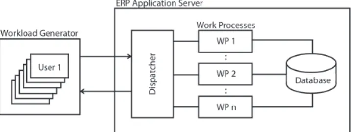
Figure 1: High-Level Overview of SAP ERP Archi-tecture

vice at another station if that server is busy doing work on behalf of another customer.

3.

SYSTEM AND MODEL DESCRIPTIONS

This section describes the architectural features of SAP ERP that are relevant for our performance modeling activ-ity. Section 3.1 gives an overview of the ERP architecture characteristics, followed in Section 3.2 by a description of the sales and distribution workload we evaluate. Section 3.3 describes the measurements used in our models and finally Section 3.4 describes the queueing models for the system.

3.1

SAP ERP Architecture

This section offers a high-level overview of the architecture of the SAP ERP system, the interested reader can find ad-ditional information in [26]. The application server is com-posed of a dispatcher and pools of separate operating system processes, called work processes, which serve requests for-warded by the dispatcher. The dispatcher assigns each re-quest to an idle work process. Service within a work process is non-preemptive. Work processes may access the database in a synchronous manner during which the work process re-mains unavailable to serve other requests due to a lack of preemptive capabilities.

Requests are served by three pools of work processes. The most important pool servesdialog steprequests, which are responsible for processing and updating information and data that are displayed on the client-side through the graph-ical user interface; this information is exchanged between client and ERP application by means of a proprietary com-munication protocol. Each dialog step request alternates cycles of CPU-intensive activities and synchronous calls to the database for data retrieval. Additionally, dialog work processes generate asynchronous calls to the database that start being served only after completion of the dialog step which requests them. These asynchronous calls are of type

update and update2 and are handled by separate pools of work processes. Update2 requests are processed at a lower priority by the platform.

Other pools of work processes exist as well, but they were not performance bottlenecks in our study. Similarly, the coordination of the whole system is performed by various components of the underlying software integration platform, such as a message server, database gateway, and shared ta-bles in memory. We do not explicitly model these compo-nents in our LQM of SAP ERP as they are not usually the primary reasons of performance degradation in the applica-tion.

3.2

Workload

In the experiments reported in the paper, we use a work-load composed by a fixed mix of sales and distribution re-quests. This mix includes transactions which describe or-der creations, oror-der listing, and delivery decisions1

. The se-quence of transactions submitted to the ERP system is iden-tical for all clients and repeated cyclically 20 times, which corresponds to an experiment duration of about 40 minutes excluding initial and final transients. The startup and warm down transients were approximately 15 minutes each.

Requests are sent to the system by a closed-loop work-load generator with emulated users that are clients for the system. Each emulated user alternates between a new dia-log step request and an exponential think time with mean

Z = 10s. A request must complete before the next think time begins. The generator is provisioned on a virtual ma-chine with one virtual CPU (vCPU). The ERP installation we have used is configured with an application server and a database server running on the same virtual machine provi-sioned with 2 vCPUs. The application server has 4 update and 1 update2 work processes. The database server could support up to 28 concurrent connections. We consider sce-narios with either 6 or 3 dialog work processes and up to 175 clients. The two virtual machines run on a host with 4-cores, each running at 2.2GHz. The host has 32GB of RAM, and 230GB of storage space. The remaining core was not assigned to any other workload.

3.3

Measurements

The SAP ERP platform includes a comprehensive mon-itoring system, accessible via the STAD _{transaction, which}

reports on resource consumption of individual transactions. Additionally, OS level metrics such as process utilizations are collected through theSAPoscol_{monitoring tool;}

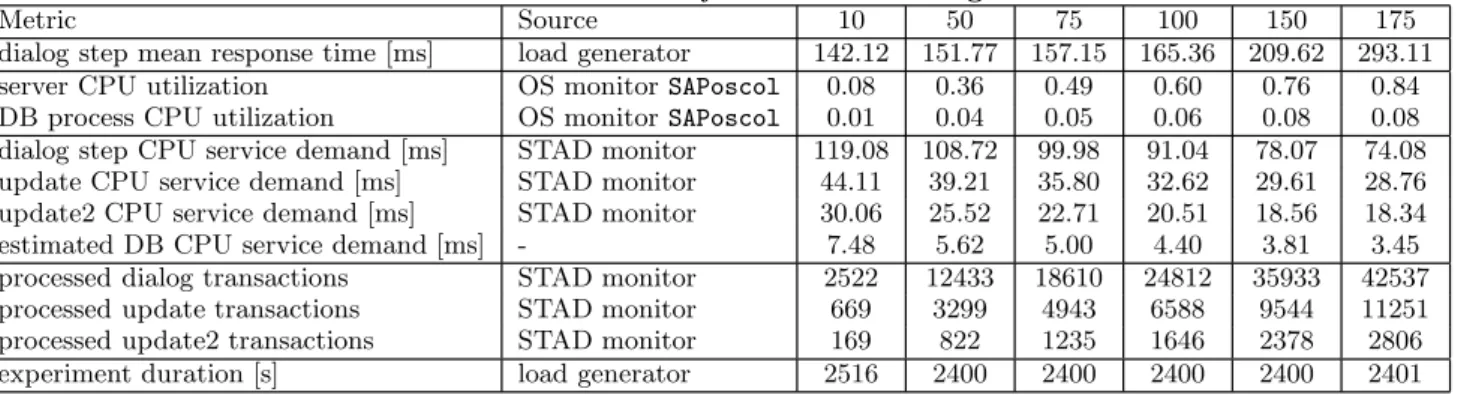
client-side measurement of response times is provided by the load generator. Table 1 gives the metrics collected and their value for different number of clientsN∈ {10,50,75,100,150,175}. Although CPU service demands are directly reported by the STAD monitoring tool for dialog, update, and update2 re-quests, we have no direct information on the service times of DB calls. We obtain these values by first multiplying the average DB process CPU utilization by the experiment du-ration and then dividing the result by the sum of the number of processed dialog steps, update, and update2 transactions. The resulting average CPU demandDdbis shown in Table 1 and it has been used as the service demand that all trans-actions place on the database server. Disk and network de-mands were not considered for this study since they were negligible in comparison to the CPU demands.

Tables 1 and 2 give the measurements obtained from the system under test. We note that the demand values in ta-bles change a great deal as the number of users increases. The demands do not differ much for the two different thread-ing levels. In each case we see the measured CPU utilization rising from 0.08 to either 0.85 or 0.84, respectively. This sug-gests that there is not a significant difference in how much CPU is used whether we operate with 6 or 3 dialog work processes. The measured response times are similar for the 1

Due to the non-disclosure agreements that are in place, we cannot provide in the paper more information on the characteristics of the individual transactions used in the ex-periment. However, we stress that these are representative of typical SAP ERP workload profiles.

two scenarios at low client population levels. However, the measured dialog response times behave differently for higher loads. For the 6 work process cases, mean response times rise to 209.62 msec and 293.11 msec for 150 and 175 clients, re-spectively. For the 3 work process cases, the response times rise to 320.32 and 473.23 msec, respectively.

Table 3 gives estimates of the demand values for the 6 work process case using a cubic spline function fitted with the demands from population 10, 100, and 175 as inputs. An asterix is next to the population levels that have estimated values. The table shows that predicting demands for a range of customer populations from a small number of measure-ments is feasible. The demand estimates, were all within 3.3% of measured values for both the 6 and 3 dialog work process cases2

.

Finally, the STAD transaction also reports on dialog step, update, and update2 response times. We found that the re-ported dialog step response times were within 12% of those reported by the workload generation tool. We report re-sponse time results as measured by the workload generation tool.

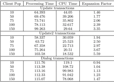
Table 4 demonstrates the impact of asynchronous messag-ing and priorities on the runtime behaviour of the system. The table gives elapsed processing time, CPU time, and an expansion factor defined as the processing time divided by CPU time for update, update2, and dialog steps as the client population increases from 10 to 150. The CPU utilization increased from approximately 8% to 76% for this popula-tion range. The update2 requests have the greatest expan-sion factor, e.g., 5.59 for 150 clients, which means that they take the longest elapsed time to have a unit of CPU demand satisfied. This is likely because update2 requests can only operate at a lower priority than other requests. However, update requests are not known to operate at a low prior-ity but they still have large expansion factors compared to dialog steps. This is because both update and update2 are scheduled asynchronously afterthe dialog step that causes them to start has completed and returned a result to the client. In the next subsection we discuss the modelling of these features in the LQM.

3.4

Queueing Models

This subsection presents a baseline product-form QNM and an LQM for the SAP ERP system under study.

3.4.1

Queueing Network Model

We begin by considering a near-product-form QNM for SAP ERP performance as a baseline model. The QNM is illustrated in Figure 2. The model is composed of a delay station that models the think times between the submission of requests. The delay station is placed in tandem with a two-server queue that represents the two vCPUs used in the experiments. Service times are assumed exponential at both stations. The system processes jobs belonging to 3 workload classes: dialog class, update class, and update2 class. The model is not strictly product-form because the classes have different mean service demands and the CPU is scheduled as first come first served.3

The population of the dialog class is 2

The estimates for the three process case are omitted to save space.

3

Such a choice was imposed on us by the tool we used to evaluate this model. However, we note that this is unlikely to qualitatively impact the conclusions of this study.

Table 1: Measurements for ERP System with 6 Dialog Work Processes

Metric Source 10 50 75 100 150 175

dialog step mean response time [ms] load generator 142.12 151.77 157.15 165.36 209.62 293.11

server CPU utilization OS monitorSAPoscol _{0.08 0.36 0.49 0.60 0.76 0.84}

DB process CPU utilization OS monitorSAPoscol 0.01 0.04 0.05 0.06 0.08 0.08

dialog step CPU service demand [ms] STAD monitor 119.08 108.72 99.98 91.04 78.07 74.08

update CPU service demand [ms] STAD monitor 44.11 39.21 35.80 32.62 29.61 28.76

update2 CPU service demand [ms] STAD monitor 30.06 25.52 22.71 20.51 18.56 18.34

estimated DB CPU service demand [ms] - 7.48 5.62 5.00 4.40 3.81 3.45

processed dialog transactions STAD monitor 2522 12433 18610 24812 35933 42537

processed update transactions STAD monitor 669 3299 4943 6588 9544 11251

processed update2 transactions STAD monitor 169 822 1235 1646 2378 2806

experiment duration [s] load generator 2516 2400 2400 2400 2400 2401

Table 2: Measurements for ERP System with 3 Dialog Work Processes

Metric Source 10 50 75 100 150 175

dialog step mean response time [ms] load generator 142.08 154.55 164.23 190.56 320.32 473.23

server CPU utilization OS monitorSAPoscol _{0.08 0.36 0.49 0.60 0.76 0.84}

DB process CPU utilization OS monitorSAPoscol _{0.01 0.03 0.04 0.05 0.06 0.07}

dialog step CPU service demand [ms] STAD monitor 119.82 109.72 100.94 92.57 79.43 74.90

update CPU service demand [ms] STAD monitor 47.92 41.94 37.82 35.21 31.02 29.74

update2 CPU service demand [ms] STAD monitor 32.98 26.81 23.11 21.11 19.18 18.34

estimated DB CPU service demand [ms] - 6.05 4.71 4.30 3.64 3.17 2.81

processed dialog transactions STAD monitor 2719 12214 18193 24696 36054 42549

processed update transactions STAD monitor 721 3248 4840 6566 9513 11268

processed update2 transactions STAD monitor 181 811 1211 1639 2371 2816

experiment duration [s] load generator 2637 2401 2401 2401 2401 2401

in the range.Ndia∈10,50,75,100,150,175; the population of the update and update2 classes in the model are estimated as Nupd =

cupd

c_diaNdia and Nupd2 = cupd2

c_dia Ndia where cupd is the number of processed update transactions andcdia is the number of processed dialog transactions as shown in Table 1. Such a choice of the populations ensures that the observed dialog, update, and update2 throughputs closely match measured values. Service demands at the vCPUs are obtained by summing the CPU and DB service demands in Table 1 for each class. Think times are chosen to be

Zdia=Zupd=Zupd2= 10 sec.

While such a model is straightforward, it does not consider software constraints such as the size of the dialog, update, and update2 work process pools and their impact on per-formance. Furthermore, it does not consider the layering of requests, priorities or asynchronous messaging behaviour and their queueing effects on performance. The purpose of LQMs is to provide a straightforward way of reflecting these features in models.

3.4.2

Layered Queueing Model

Figure 3 illustrates the LQM for the SAP ERP platform. Table 1 gives the service demand parameters for the layered queueing model for the system under study for the 6 dialog work process scenario. The parameters are summarized per dialog step request.

The model reflects the workload generator’s emulated users that submit requests to the application server of Figure 1. Emulated users are represented as clients that generate syn-chronous dialog requests to a pool of dialog work processes. The dialog processes have two phases of service. The first phase (P1) corresponds to executing business logic. It

al-Figure 2: QNM for an ERP Application Server ternates between using the vCPU and making synchronous calls to the database service, afterwards the client is released. The second phase (P2) causes asynchronous requests to the update and update2 pools of work processes. This is because in the ERP platform update requests are processed after the dialog step completes. A client’s dialog request does not typically incur any contention for the vCPU due to its own asynchronous update requests. All three types of work processes make synchronous visits to the database service. Client think times are illustrated as a visit to a delay centre named Think. The update2 processes access the vCPU at a lower priority than all other processes. The process pool

Table 3: Estimated Demands for ERP System with 6 Dialog Work Processes using Cubic Splines with Data for 10, 100, and 175 clients

Metric 10 *50 *75 100 *150 175

dialog step CPU service demand [ms] 119.08 105.87 98.11 91.04 79.30 74.08 update CPU service demand [ms] 44.11 39.21 35.80 32.62 29.61 28.76 update2 CPU service demand [ms] 30.06 25.14 22.51 20.51 18.68 18.34 estimated DB CPU service demand [ms] 7.48 5.92 5.08 4.40 3.66 3.45

Figure 3: LQM for an ERP Application Server

sizes used in the model correspond to the ERP application’s configuration settings as discussed in Section 3.2. Note that the dispatcher for work processes is not represented explic-itly as a software server in this model because it did not seem to have a significant impact on performance in our study.

In Figure 3, the numbers on the arrows flowing into an entity describe the number of visits to that entity by other entities in the model. The visit counts follow directly from the nature of interactions between clients, dialog work pro-cesses, update work propro-cesses, update2 work propro-cesses, the database service, the vCPUs and the Think delay centre. In particular, the relative number of visits to update and up-date2 processes are based on the counts of processed trans-actions as shown in the Tables 1 and 2. We also note that the second phase of processing hasnear-zero demands on the vCPU. Small non-zero demands are required by the MOL tool as an artifact of its assumption of a central server model for each phase of processing.

The impacts of the pools of work processes and the dual cores associated with the ERP VM are reflected in the LQM using multi-server queueing centres [24]. Asynchronous mes-saging is captured in the LQM using the residence time ex-pressions described in previous work [29]. Priority schedul-ing is implemented accordschedul-ing the method by Bryant et al. [7]. Two phases of processing are implemented in LQMs accord-ing to the residence time expressions devised previously [31] but adapted for use within the closed queueing model ap-proach of the MOL tool.

4.

MODELLING RESULTS

This section presents the results for the QNM and LQM models.

Table 4: Impact of Asynchronous Messaging and Priorities on Expansion Factor

Client Pop Processing Time CPU Time Expansion Factor Update transactions 10 64.393 44.05 1.46 50 69.476 39.206 1.77 75 73.741 35.802 2.06 100 78.113 32.617 2.39 150 99.263 29.64 3.35 Update2 transactions 10 58.337 30.059 1.94 50 63.72 25.523 2.50 75 67.358 22.713 2.97 100 75.264 20.51 3.67 150 103.58 18.532 5.59 Dialog transactions 10 111.76 119.1 0.94 50 113.38 108.72 1.04 75 113.16 99.983 1.13 100 112.33 91.042 1.23 150 115.07 78.068 1.47

4.1

QNM Results

We begin with the results of the QNM for SAP ERP. The predictions for CPU utilization and dialog step response times are computed using a QNM simulator [4]. The results are given in Table 5 together with the values ofNdia,Nupd, andNupd2 used in the model. Note that response times are not monotonically increasing with the total population be-cause the measured service demands change under increas-ing population values. The results in the table indicate that the QNM is effective at predicting CPU utilization, with a maximum error of 10% forNdia= 175. However, when we look at the more challenging problem of matching the mean dialog response time we see that a basic QNM grossly un-derestimates the actual response times. In particular, for

Ndia = 175 the predicted response time (165.00 msec) is significantly less than the measured value for the SAP ERP system (293.11 msec). Errors of similar magnitude are in-curred for all but low load populations. Our interpretation is that the inaccuracies are the result of ignoring the effects of worker process pool sizes and other software system proper-ties such as prioriproper-ties and asynchronous messaging behavior. Summarizing, the results of this subsection indicate that a basic application of QNMs cannot be used reliably for es-timating fundamental performance metrics of the SAP ERP system such as end-to-end response times. Utilization can be predicted well, but this is in general much easier to match than response times in presence of large think times such as in the present case study. In the next section we show how a LQM can greatly enhance the predictive capabilities when applied to complex software systems such as the SAP ERP system.

Table 5: QNM Mean Dialog Response Times and Utilization for 6 Dialog Work Processes Case

Measured Measured QNM (MVA)

Pop CPU U DialogResp Dialog Pop. Update Pop. Update2 Pop. CPU Util DialogResp

10 0.08 142.12 10 3 1 0.07 127.03 50 0.36 151.77 50 13 3 0.32 125.20 75 0.49 157.15 75 20 5 0.44 126.65 100 0.60 165.36 100 27 7 0.53 128.30 150 0.76 209.62 150 40 10 0.68 144.61 175 0.85 293.11 175 46 12 0.75 165.00

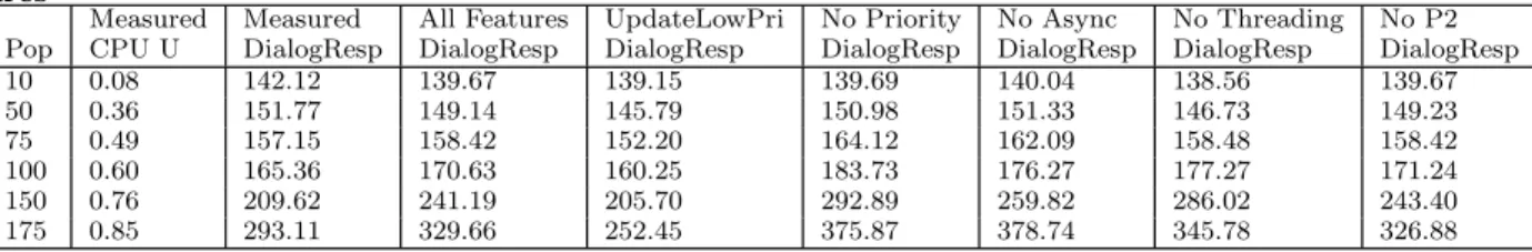
Table 6: LQM mean dialog response times for 6 dialog workprocess case with all features and excluded features

Measured Measured All Features UpdateLowPri No Priority No Async No Threading No P2 Pop CPU U DialogResp DialogResp DialogResp DialogResp DialogResp DialogResp DialogResp

10 0.08 142.12 139.67 139.15 139.69 140.04 138.56 139.67 50 0.36 151.77 149.14 145.79 150.98 151.33 146.73 149.23 75 0.49 157.15 158.42 152.20 164.12 162.09 158.48 158.42 100 0.60 165.36 170.63 160.25 183.73 176.27 177.27 171.24 150 0.76 209.62 241.19 205.70 292.89 259.82 286.02 243.40 175 0.85 293.11 329.66 252.45 375.87 378.74 345.78 326.88

4.2

LQM results

We now consider the following sets of results for the LQM model introduced in Section 3.4.2. Tables 6 and 7 give the results for the six and three dialog work process cases, re-spectively, for the following scenarios: where all modelling features are included (All features) as per Section 3.4.2; the update processes also run at a low priority as well as the update2 processes (UpdateLowPri); all processes run at the same priority (No Pri); where asynchronous calls are made to be synchronous calls (No Async); where threading levels are set to high values so there is no queueing for software processes (No Thread); and where the second phase of pro-cessing is included in the first phase (No P2). We note that only one modelling feature is changed at a time. Each case includes all the features or differs from the (All features) case by only one feature. Tables 8 and 9 give the results for the cases where all features are included but demands are estimated through cubic splines as shown in Table 3.

Tables 6 and Table 7 give measured and predicted mean dialog step response times for the 6 and 3 dialog work process case with between 10 and 175 customers, respectively. As mentioned previously, the response time behaviour of the system for the 3 work process case and the 6 work process case differ significantly for higher numbers of clients. For 150 and 175 clients, the 3 work process results are approximately 100 and 180 msec higher than for the 6 dialog process case, respectively.

From Table 6 and Table 7 we see that the mean response times predicted by the LQM for the (All features) case match the measured values closely. The greatest error for the 6 work process case is 15% at 150 clients. The greatest error for the 3 work process case is 24%, for the 175 client case. For the 150 client case, the LQM predicted a mean response time that is approximately 90 msec greater for the 3 dialog process case than the 6 dialog process case. Similarly, for the 175 client case, the LQM estimated mean response time for the 3 dialog process case is greater than that of the 6 dialog process case by approximately 260 msec. In effect, the LQM prediction is very close for 150 clients, but it over-estimates the degradation for 175 clients. We note that the model is very accurate for CPU utilizations of 76% and less

for both the 6 and 3 dialog process cases which is already a high utilization for a production enterprise application en-vironment. The LQM also predicts the smaller increases in response times for client populations of 50, 75, and 100 that result when decreasing the number of dialog processes from 6 to 3.

We now consider disabling one feature at a time from the LQM. The following results are from Tables 6 and Table 7. First, we consider modelling the update processes at a low priority (UpdateLowPri) in addition to the update2 pro-cesses. This hides more of the update work from the clients and as a result response times drop. This seems advanta-geous for the 6 work process case but becomes too optimistic for the 3 work process case. Next, we consider disabling the use of priorities (No Priority). The results become pes-simistic for the 6 dialog process case and very pespes-simistic for the 3 dialog process case. In the subsequent scenario we make all calls synchronous (No Async). The results be-come slightly pessimistic for the 6 dialog process case, but very pessimistic for the 3 dialog process case. To further consider the impact of dialog process pool size (No Thread) we increase the pool sizes in the model to match the num-ber of clients. As expected we end up with predictions that are very similar for the 6 and 3 dialog process cases, differ-ences are due to slightly different measured demands for the these two scenarios. Clearly, without the threading feature for modelling pool size we are not able to distinguish the impact of pool size. Finally, we consider the model without the second phase of processing (No P2). In this scenario the calls to update processes are made in the first phase, which from the analytic model’s perspective permits a dialog re-quest to compete for CPU resources with its own update requests. Note that update2 requests run at a low priority. In this scenario we see the mean response times for both the 6 and 3 dialog work process cases increase slightly, but enough to show that support for a second phase of process-ing is advantageous especially at high load.

To summarize, for measured CPU utilizations of 76% or less the LQM offered mean dialog step response time pre-dictions very close to measured values. The greatest error for the 6 and 3 work process cases for this utilization limit was 15% for the 6 work process case at 150 clients. When

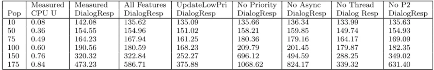
Table 7: LQM mean dialog response time results for 3 dialog work process case with all features and excluded features

Measured Measured All Features UpdateLowPri No Priority No Async No Thread No P2 Pop CPU U DialogResp DialogResp DialogResp DialogResp DialogResp Dialog Resp DialogResp

10 0.08 142.08 135.62 135.09 135.66 136.34 133.99 135.63 50 0.36 154.55 154.96 151.02 158.21 159.85 149.74 154.93 75 0.49 164.23 167.94 161.25 180.36 179.16 164.17 169.09 100 0.60 190.56 180.59 168.23 209.79 201.45 179.87 182.35 150 0.76 320.32 322.84 252.27 696.12 494.59 288.25 349.02 175 0.84 473.23 586.71 375.88 1068.62 824.17 339.32 631.40

Table 8: LQM mean dialog response times for 6 dia-log work process case with all features and estimated demands

Measured Measured All Features Pop CPU U DialogResp DialogResp 10 0.08 142.12 139.67 50 0.36 151.77 149.10 75 0.49 157.15 158.16 100 0.60 165.36 170.63 150 0.76 209.62 239.86 175 0.85 293.11 316.44

disabling features one at a time the greatest errors across the 6 and 3 work process cases were: (UpdateLowPri, 24%), (No Priority, 117%), (No Async, 29%), (No Thread, 36%), and (No P2, 16%). This shows the advantages of using the non-product-form features.

Table 8 and 9 provide results for LQMs with all modelling features included but with demands estimated using cubic splines, as in Table 3. The response time predictions match the measured response times closely showing that demand measurements from a small set of client population levels can be used to estimate the demands at other client population levels effectively.

5.

SUMMARY AND CONCLUSIONS

The results of our study show that non-product-form fea-tures such as priority scheduling, asyncrhonous messaging, and the layered use of servers with finite numbers of work processes are all important for modelling the production en-terprise application platform under study. The use of a sec-ond phase of processing for dialog requests also improved re-sponse time predictions. The LQM offered mean dialog step response time predictions within 15% of measured values for a wide range of load levels. When disabling key features one at a time the greatest errors across the 6 and 3 work pro-cess cases were: (No Priority, 117%), (No Async, 54%), (No Thread, 36%). Thus if priorities, asynchronous processing

Table 9: LQM mean dialog response time results for 3 dialog workprocess case with all features and estimated demands

Measured Measured All Features Pop CPU U DialogResp DialogResp 10 0.08 142.08 135.62 50 0.36 154.55 154.43 75 0.49 164.23 167.35 100 0.60 190.56 180.59 150 0.76 320.32 324.31 175 0.84 473.23 586.71

or threading support for pool sizes are not included in the model response time estimates can differ from measured val-ues by 36% to 117%. This shows the advantages of using the non-product form features.

We observed that measured demand values changed sig-nificantly from one population to another, yet given the de-mands for a low, medium, and high population level, a cu-bic spline did a very good job at estimating the demands of intermediate populations. Measured demand values for different threading levels did not change much. Use of the estimated demands did not significantly affect the predictive accuracy of the model.

Analytic models are favoured for runtime optimization be-cause they provide fast solutions for even large systems com-pared to other techniques. The MOL tool offered solutions for each of the models considered in this paper in a fraction of a second on a laptop. This suggests that the approach could be used to support runtime optimization methods.

Our one concern about applying these methods at run-time follows from our experience in validating the models. We found it necessary to collect data for fourty minutes to properly characterize steady state conditions and a mean dialog response time via measurement. Measurements of mean dialog response time from shorter time periods may differ more significantly from the the predictions which cor-respond to the steady state. At runtime, we expect that such models are best used to determine the likely impact of changes to a system on application behaviour rather than to predict mean response times over short time scales that may be significantly affected by transient behaviour.

Our future work includes more validation exercises for the ERP application and other platforms. We plan to consider a greater variety of more controlled workloads and to integrate the approach into a runtime management system for the platform in infrastructure as a service environments.

6.

ACKNOWLEDGEMENTS

This research has been partially funded by the InvestNI/SAP MORE project.

7.

REFERENCES

[1] C. Amza, A. Chanda, A. Cox, S. Elnikety, R. Gil, K. Rajamani, and W. Zwaenepoel. Specification and implementation of dynamic web site benchmarks. InProc. of International Workshop on Workload Characterization, pages 863–867, 2002.

[2] D. Ardagna, C. Ghezzi, and R. Mirandola. Rethinking the use of models in software architecture.Quality of Software Architectures. Models and Architectures, 1–27, 2008. [3] F. Baskett, K. M. Chandy, R. R. Muntz, and F. G.

Palacios. Open, closed, and mixed networks of queues with different classes of customers.Journal of the ACM, 22(2):248–260, 1975.

[4] M. Bertoli, G. Casale, and G. Serazzi. JMT: performance engineering tools for system modelling.ACM

SIGMETRICS Performance Evaluation Review, 36(4):248–260, 2009.

[5] TPC-W Benchmark.http://www.tpc.org/tpcw/default.asp. [6] G. Bolch, S. Greiner, H. de Meer, and K. S. Trivedi.

Queueing Networks and Markov Chains. 2nd ed., John Wiley and Sons, 2006.

[7] R. Bryant, A. Krzesinski, and P. Teunissen. The MVA pre-empt resume priority approximation. InSIGMETRICS ’83: Proceedings of the 1983 ACM SIGMETRICS conference on Measurement and modelling of computer systems, pages 12–27, New York, NY, USA, 1983. ACM. [8] K. M. Chandy and D. Neuse. Linearizer: A heuristic

algorithm for queuing network models of computing systems.Comm. of the ACM, 25(2):126–134, 1982. [9] Y. Chen, S. Iyer, X. Liu, D. Milojicic, and A. Sahai.

Translating service level objectives to lower level policies for multi-tier services.Cluster Computing, 11(3):299–311, 2008. [10] P. Cremonesi, P. J. Schweitzer, and G. Serazzi. A unifying

framework for the approximate solution of closed multiclass queuing networks.IEEE Trans. on Computers,

51:1423–1434, 2002.

[11] G. Franks, T. Omari, C. M. Woodside, O. Das, and S. Derisavi. Enhanced modelling and solution of layered queueing networks.IEEE Trans. Software Engineering, 35(2):148–161, 2009.

[12] G. Franks, C. Woodside, and J. Rolia. Multi-threaded servers with high service time variation for layered queueing networks. In E. Gelenbe, editor,Computer System Performance modelling in Perspective - A Tribute to the Work of Professor Kenneth C. Sevcik, volume 1 of Advances in Computer Science and Engineering. Imperial College Press, 2006.

[13] M. Goldszmidt, I. Cohen, R. Powers, and R. Powers. Short term performance forecasting in enterprise systems. InIn ACM SIGKDD Intl. Conf. on Knowledge Discovery and Data Mining, pages 801–807. ACM Press, 2005. [14] U. Herzog and J. Rolia. Performance validation tools for

software/hardware systems.Performance Evaluation Journal, 45(2), 2001.

[15] M. Huebscher and J. McCann. Simulation model for self-adaptive applications in pervasive computing. InProc. of Database and Expert Systems Applications, pages 694–698, Aug 2004.

[16] P. Jacobson and E. Lazowska. Analysing queueing networks with simultaneous resource possession.CACM, pages 141–152, Feb 1982.

[17] E. D. Lazowska, J. Zahorjan, G. S. Graham, and K. C. Sevcik.Quantitative System Performance. Prentice-Hall, 1984.

[18] Y. Lu, T. Abdelzaher, C. Lu, L. Sha, and X. Liu. Feedback control with queueing-theoretic prediction for relative delay guarantees in web servers. InProc. of the IEEE Real-Time and Embedded Technology and Applications Symposium, page 208, 2003.

[19] D. Menasce. Two-level iterative queuing modelling of software contention. InProc. of the IEEE International Symposium on modelling, Analysis, and Simulation of Computer and Telecommunications Systems (MASCOTS), page 267, 2002.

[20] D. Menasce and M. Bennani. Analytic performance models for single class and multiple class multithreaded software servers. InProc. of the International Computer

Measurement Group (CMG) Conference, pages 475–482, 2006.

[21] M. Molloy. Performance analysis using stochastic petri nets.

IEEE Transactions on Computers, 31:913–917, 1982. [22] T. Omari, G. Franks, M. Woodside, and A. Pan. Efficient

performance models for layered server systems with replicated servers and parallel behavior.Journal of Systems

and Software, 80(4):510–527, April 2007.

[23] J. Rolia.Performance estimates for multi-tasking software systems. M.Sc. Thesis, University of Toronto, 1987. [24] J. A. Rolia and K. C. Sevcik. The method of layers.IEEE

Trans. on Software Engineering, 21(8):689–700, 1995. [25] W. Sanders, W. O. II, M. Qureshi, and F. Widjanarko. The

ultrasan modelling environment.Performance Evaluation, 24:89–115, 1995.

[26] T. Schneider.SAP Performance Optimization Guide. SAP Press, 2003.

[27] A. Seidmann, P. J. Schweitzer, and S. Shalev-Oren. Computerized closed queueing network models of flexible manufacturing systems.Large Scale Systems, 12:91–107, 1987.

[28] K. C. Sevcik. Priority scheduling disciplines in queuing network models of computer systems. InIFIP Congress, pages 565–570, 1977.

[29] F. Sheihk, J. Rolia, P. Garg, S. Frolund, and A. Shepherd. Layered modelling of large-scale distributed applications. In

Proc. of First World Congress on Systems Simulation, Quality of Service modelling, pages 247–254, Sept 1997. [30] B. Urgaonkar, G. Pacifici, P. J. Shenoy, M. Spreitzer, and

A. N. Tantawi. An analytical model for multi-tier internet services and its applications. InProc. of ACM

SIGMETRICS, pages 291–302. ACM Press, 2005.

[31] C. Woodside, J. Neilson, D. Petriu, and S. Majumdar. The stochastic rendezvous network model for performance of synchronous client-server-like distributed software.IEEE Trans. Computer, 44:20–34, 1995.

[32] M. Woodside, T. Zhen, and M. Litoiu. Service system resource management based on a tracked layered performance model. InProc. of the International