Low-rank matrix estimation in multi-response regression
with measurement errors: Statistical and computational
guarantees
Xin Li
1and Dongya Wu
21
School of Mathematics, Northwest University, Xi’an, 710069, P. R. China
2School of Information Science and Technology, Northwest University, Xi’an,
710069, P. R. China
Abstract
In this paper, we investigate the matrix estimation problem in multi-response regres-sion with measurement errors. A nonconvex error-corrected estimator is proposed to estimate the matrix parameter via a combination of the loss function and the nuclear norm regularization. Then under the low-rank constraint, we analyse the statistical and computational theoretical properties of global solution of the nonconvex regularized es-timator from a general point. In the statistical aspect, we establish the recovery bound for the global solution of the nonconvex estimator, under restricted strong convexity on the loss function. In the computational aspect, we solve the nonconvex optimization problem via the proximal gradient method. The algorithm is proved to converge to a near-global solution and achieve a linear convergence rate. In addition, we also establish sufficient conditions for the general results to be held for specific types of corruptions, including the additive noise and missing data. Probabilistic consequences are obtained by applying the general results. Finally, we demonstrate our theoretical consequences by several numerical experiments on the corrupted errors-in-variables multi-response re-gression models. Simulation results show remarkable consistency with our theory under high-dimensional scaling.
Keywords: Low-rank matrix; Measurement error; Nonconvex estimation; Recovery bound; Statistical consistency; Proximal gradient method; Convergence rate
1
Introduction
Massive data sets have posed a variety of challenges to the field of statistics and machine learning in recent decades. In view of these challenges, researchers have developed different classes of statistical models to deal with the complexities of modern data, such as sparse linear regression models, matrix regression models with rank constraints, graphical models and various nonparametric models. Effective estimation methods based on convex or nonconvex optimization problems have also been proposed to analyse these models from both statistical
and computational aspects. By now, high-dimensional statistics have gained fruitful results and have been successfully used in a wide range of application fields; see the books [9, 30] for an overall review.
In standard formulations of statistical inference problems, it is assumed that the collected data are clean enough, meaning that there exists no measurement error. However, this hy-pothesis is neither realistic nor reasonable, since in many real-world problems, due to the instrumental constraint or the lack of observation, the collected data, such as human genetic data, may always be corrupted and tend to be noisy or partially missing, indicating that measurement error cannot be avoided in general. There have been a variety of researches focusing on models with corrupted data for regression problems; see, e.g., [6, 10, 27] and refer-ences therein. However, much of the previous theoretical work is for classical low-dimensional statistics, that is, the sample size n diverges while the problem dimension d is fixed. As for the high-dimensional scenario (i.e., n d), authors in [25] pointed out that misleading in-ference results can still only be obtained if the method for clean data is applied naively to the corrupted data. Thus it is necessary to take measurement errors into consideration and develop new error-corrected methods for high-dimensional models.
Recently, some regularization methods have been proposed to deal with high-dimensional errors-in-variables regression. For example, in [17], Loh and Wainwright proposed a nonconvex Lasso-type estimator via substituting the corrupted Gram matrix with unbiased surrogates for additive and missing data cases, and established the statistical errors for global solutions. Later in [19], the authors further extended the `1-norm regularizer to the nonconvex regularizers,
namely SCAD and MCP, and investigate liner and logistic regression models. Then in order to avoid the nonconvexity, Datta and Zou developed the convex conditional Lasso (CoCoLasso) by defining the nearest positive semi-definite matrix in [12]. The CoCoLasso thus enjoys the benefits of convex optimization and is shown to possess nice estimation accuracy in linear regression. Rosenbaum and Tsybakov [23] worked on the sparse linear model with corrupted covariates, and proposed a modified form of the Dantzig selector, called matrix uncertainty selector (MUS). The MUS is proved to be variable selection consistency under strong conditions while the consistency for parameter estimation is not guaranteed. Further development of the method MUS included modification to obtain statistical consistency, and generalization to handle the cases of unbounded and dependent measurement errors as well as the generalized linear models [4, 5, 24, 26].
There are some methods fall out the category of regularization methods. For instance, au-thors in [14] first performed model selection and then made use of the corrected least squares on the reduced model for estimation; Chen and Caramanis [11] modified the orthogonal matching pursuit algorithm for variable selection in errors-in-variables linear regression; the measure-ment error boosting (MEBoost) algorithm [8] was based on the idea of classical estimation equation and implemented measurement error corrected variable selection at every iterative path.
However, the aforementioned researches mainly focused on the high-dimensional errors-in-variables regression with univariate responses, and relatively little attention is paid for the case of multivariate responses, a model which is also an special and important instance of matrix regression [29]. Though a simple and natural idea is to vectorize both the response matrix and the coefficient matrix so that methods for univariate response case can be directly applied, it may ignore the particular low-dimensional structures of the coefficient matrix such as low rankness and row/column sparsity as well as the multivariate nature of the responses
[13]. Moreover, the multi-response linear regression has a substantial wider application than that of the univariate case in modern large-scale association analysis, such as genome-wide association studies [15] and social network analyses. Therefore, in this work, we shall deal with the multi-response case in the high-dimensional errors-in-variables regression. More precisely, we shall consider the multi-response regression model Y = XΘ∗ +, where Θ∗ ∈ Rd1×d2 is
the unknown underlying matrix parameter. The covariate matrixX does not need to be fully observed, instead, two types of corruption will be discussed, including the additive noise and missing data cases.
The major contributions of this paper areas follows. First, we develop a new error-corrected method for estimating the parameter Θ∗. Then in the statistical aspect, under the low-rank assumption on the true parameter Θ∗, we provide the squared`2recovery bound for any global
solution ˆΘ of the optimization problem as kΘˆ −Θ∗k2
2 = O(λ2−qRq); see Theorem 1. In the
aspect of computation, we apply the proximal gradient method [21] to solve a modified version of the optimization problem. The algorithm is proved to converge linearly to a near-global solution of the nonconvex regularized problem; see Theorem 2. Apart from the general and deterministic results, i.e., Theorems 1 and 2, in addition, we also discuss probabilistic conse-quences for the additive noise and missing data cases by establishing sufficient conditions for the general results to be held; see Corollaries 1–4. Numerical experiments are also performed to demonstrate the consequences.
The remainder of the article is organized as follows. In Section 2, we provide background on the high-dimensional multi-response regression model with measurement errors and then propose a novel error-corrected estimator. Some regularity conditions are also imposed to facilitate the following analysis. In Section 3, we establish our main results on statistical consistency and algorithmic rate of convergence. In Section 4, probabilistic consequences for specific corruption models are obtained by verifying the required regularity conditions. In Section 5, we perform several numerical experiments to demonstrate statistical and compu-tational results. Conclusions and future work are discussed in Section ??. Technical lemmas are presented in Appendix.
We end this section by introducing some useful notations. For d ≥ 1, let Id stand for
the d ×d identity matrix. For a matrix X ∈ Rn×d, let X
ij (i = 1, . . . , n, j = 1,2,· · · , d)
denote its ij-th entry, Xi· (i = 1, . . . , n) denote its i-th row, X·j (j = 1,2,· · · , d) denote
its j-th column, and diag(X) stand for the diagonal matrix with its diagonal entries equal to X11, X22,· · · , Xdd. We write λmin(X) and λmax(X) to denote the minimal and maximum
eigenvalues of a matrix X, respectively. For a matrix Θ ∈Rd1×d2, we define d= min{d
1, d2},
and denote its ordered singular values by σ1(Θ) ≥ σ2(Θ) ≥ · · ·σd(Θ) ≥ 0. We use |||·|||
to denote different types of matrix norms based on singular values, including the nuclear norm |||Θ|||∗ =Pd
j=1σj(Θ), the spectral or operator norm|||Θ|||op =σ1(Θ), and the Frobenius
norm |||Θ|||F = ptrace(Θ>Θ) = qPd
j=1σj2(Θ). For a pair of matrices Θ and Γ with equal
dimensions, we let hhΘ,Γii= trace(Θ>Γ) denote the trace inner product on matrix space. For a function f :Rd→R,∇f is used to denote a gradient or subgradient depending on whether
2
Problem setup
In this section, we begin with background on the high-dimensional errors-in-variables multi-response regression, and then a precise description on the proposed error-corrected estimation methods. Finally, we introduce some regularity conditions that will facilitate the following analysis.
2.1
Model setting
Consider the high-dimensional multi-response regression model which links the response vector
Yi·∈Rd2 to a covariate vector Xi·∈Rd1
Yi· = Θ∗>Xi·+i· for i= 1,2,· · · , n, (1)
where Θ∗ ∈ Rd1×d2 is the unknown parameter matrix,
i· ∈ Rd2 is the observation noise
independent of Xi·. Model (1) can be written in a more compact form using matrix notation.
Particularly, define the multi-response matrix Y = (Y1·, Y2·,· · · , Yn·)> ∈ Rn×d2 with similar
definitions for the covariate matrix X ∈ Rn×d1 (n d
1) and the noise matrix ∈ Rn×d2 in
terms of {Xi·}ni=1 and {i·}ni=1, respectively. Then model (1) is re-written as
Y =XΘ∗+. (2)
We work within a high-dimensional framework which allows the number of covariates d2
to grow and possibly more than the sample size n in this paper. It is already known that consistent estimation cannot be obtained when n d1 unless the model is imposed with
additional structure, such as low-rankness in the matrix estimation problems. In the following, unless otherwise specified, Θ∗ ∈Rd1×d2 is assumed to be of either exactly low-rank, i.e., it has
rank far less than min{d1, d2}, or near low-rank, meaning that it can be approximated by a
matrix of low-rank perfectly. One popular way to measure the degree of low-rank is to use the matrix `q-ball (Accurately speaking, when q ∈[0,1), these sets are not real “ball”s , as they
fail to be convex), which is defined as, for q ∈[0,1], and a radius Rq >0,
Bq(Rq) := {Θ∈Rd1×d2 d X i=1 |σi(Θ)|q≤Rq}, (3)
whered= min{d1, d2}. Note that the`0 matrix ball corresponds to the case of exact low-rank,
meaning rank at most R0; while the `q matrix ball for q ∈ (0,1] corresponds to the case of
near low-rank, which enforces a certain decay rate on the ordered of the singular values of the matrix Θ ∈ Bq(Rq). In this paper, we fix q ∈ [0,1], and assume that the true parameter
Θ∗ ∈Bq(Rq) unless otherwise specified.
In standard formulations, the true covariatesXi·’s are assumed to be fully-observed.
How-ever, this assumption is not realistic for many real-world applications, in which the covariates may be observed with measurement errors, and we use Zi·’s to denote corrupted versions
of the corresponding Xi·’s. Zi· is usually assumed to be linked to Xi· via some conditional
distribution as follows
Zi· ∼Q(·|Xi·) for i= 1,2,· · · , n. (4)
As has been discussed in previous literatures (e.g., [17, 19]), there are mainly two types of corruption:
(a) Additive errors: For each i = 1,2,· · · , n, we observe Zi· = Xi·+Wi·, where Wi· ∈ Rd1 is
a random vector independent of Xi· with mean 0and known covariance matrix Σw.
(b) Missing data: For each i = 1,2,· · · , n, we observe a random vector Zi· ∈Rd1, such that
for each j = 1,2· · · , d1, we independently observe Zij =Xij with probability 1−ρ, and
Zij = 0 with probability ρ, where ρ∈[0,1).
Throughout this paper, we assume a Gaussian model on the covariate and error matrices. Specifically, the matrices X, W and are assumed to be random matrices with independent and identically distributed (i.i.d.) rows as sampled from Gaussian distributions N(0,Σx),
N(0, σw2Id1) and N(0, σ
2
Id2), respectively. Then one has that Σw =σ
2
wId1.
Define Z = (Z1·, Z2·,· · · , Zn·)>. Then Z is the observed covariate matrix, which involves
certain types of measurement error, and will be specified according to the context.
2.2
Error-corrected M-estimators
When there exists no measurement error, meaning that the covariate matrix X is correctly obtained, previous literatures have proposed various methods for the rank-constrained prob-lems; see, e.g., [20, 22, 31] and references therein. Most of the estimators are formulated as solutions to certain semidefinite programs (SDPs) based on the nuclear norm regular-ization. Recall that for a matrix Θ ∈ Rd1×d2, the nuclear or trace norm is defined by
|||Θ|||∗ = Pd
j=1σj(Θ) (d = min{d1, d2}), corresponding to the sum of its singular values.
For instance, given model (2), defineN =nd2, a commonly-used estimator is based on solving
the following SDP: ˆ Θ∈arg min Θ∈S 1 2N|||Y −XΘ||| 2 F +λNkΘk∗ , (5)
where S is a subset of Rd1×d2, andλ
N >0 is a regularization parameter. The nuclear norm of
a matrix offers a natural convex relaxation of the rank constraint, analogous to the `1-norm as
a convex relaxation of the cardinality of a vector. The statistical and computational property of the nuclear norm as a regularizer has been studied deeply and applied widely in various fields, such as matrix completion, matrix decomposition and so on. Apart from the nuclear norm, other regularizers including the elastic net, SCAD and MCP, which were first proposed to solve sparse recovery problem in linear regression, have also been used in low-rank matrix estimation problem; see [31] for a detailed investigation.
Note that (5) can be re-written as follows ˆ Θ∈arg min Θ∈S 1 2NhhX >XΘ,Θii − 1 NhhX >Y,Θii+λ N|||Θ|||∗ . (6)
Recall the relation N =nd2, the SDP optimization problem (6) is transformed to
ˆ Θ∈arg min Θ∈S 1 d2 1 2nhhX >XΘ,Θii − 1 nhhX >Y,Θii+λ n|||Θ|||∗ , (7)
where we have defined λn = d2λN. In the case of measurement errors, the quantities X
>X
n
and X>nY are both unknown, which means that this estimator does not work. However, this transformation still provides some useful intuition for estimation via the plug-in principle.
Specifically, given a set of samples, one way is to find suitable estimates of the quantities X>nX and X>nY that are adapted to the cases of additive noise and/or missing data.
Let (ˆΓ,Υ) denote estimates of (ˆ X>nX,X>nY). Inspired by (7) and ignoring the constant, we propose the following estimator to solve the low-rank estimation problem in the measurement error case: ˆ Θ∈arg min Θ∈S 1 2hh ˆ ΓΘ,Θii − hhΥˆ,Θii+λ|||Θ|||∗ , (8)
whereλis the regularization parameter. The feasible region is specialized asS ={Θ∈Rd1×d2 :
|||Θ|||∗ ≤ ω}, and the parameter ω > 0 must be chosen carefully to guarantee Θ∗ ∈ S. We include this side constraint is because of the nonconvex nature of the estimator, which will be explained in detail in the following. Then any matrix Θ ∈ S will also satisfy |||Θ|||∗ ≤ω, and since the optimization subject function is continuous, it is guaranteed by Weierstrass extreme value theorem that a global solution ˆΘ always exists.
Note that the estimator (8) is just a general expression, and concrete values for (ˆΓ,Υ) stillˆ need to be determined. For the specific additive noise and missing data cases, as discussed in [17], an unbiased choice of the pair (ˆΓ,Υ) is given respectively byˆ
ˆ Γadd := Z>Z n −Σw and Υˆadd := Z>Y n , (9) ˆ Γmis := ˜ Z>Z˜ n −ρ·diag ˜ Z>Z˜ n ! and Υˆmis := ˜ Z>Y n ˜ Z = Z 1−ρ . (10)
In the high-dimensional regime (n d1), the matrices ˆΓadd and ˆΓmis in (9) and (10) are
always negative definite; indeed, both the matrices Z>Z and ˜Z>Z˜ are with rank at most
n, and then the positive definite matrices Σw and ρ·diag
˜
Z>Z˜ n
are subtracted to arrive at the estimates ˆΓadd and ˆΓmis, respectively. Therefore, the above estimator (8) involves solving
a nonconvex optimization problem. Due to the nonconvexity, it is generally impossible to obtain a global solution through a polynomial-time algorithm. Nevertheless, this issue is not significant in our setting, and we shall establish that a simple proximal gradient algorithm converges linearly to a matrix extremely close to any global optimum of the problem (8) with high probability.
2.3
Regularity conditions
Now we impose some regularity conditions on the surrogate matrices ˆΓ and ˆΥ, which will be beneficial to the statistical and computational analysis for the estimator (8).
In high-dimensional linear regression with univariate responses (i.e., d2 = 1), when the
true covariate matrix X is correctly obtained, it is well understood that a type of restricted eigenvalue condition (REC) is sufficient to guarantee nice `2 recovery for the Lasso; see, e.g.,
[7, 28]. The REC then was utilized to establish `2 recovery bound in the errors-in-variables
linear regression [17]. More general conditions called restricted strong convexity/smoothness (RSC/RSM) have also been adopted in the analysis of matrix regression, and is applicable when the loss function is nonquadratic or nonconvex; see, e.g., [16, 19, 20]. In this paper, the following RSC/RSM conditions are required.
Definition 1. [Restricted strong convexity] The matrix Γˆ is said to satisfy a restricted strong convexity with curvature α1 >0 and tolerance τ(n, d1, d2)>0 if
hhΓ∆ˆ ,∆ii ≥α1|||∆|||F2 −τ|||∆|||2∗ for all ∆∈R
d1×d2. (11)
Definition 2. [Restricted strong smoothness] The matrixΓˆ is said to satisfy a restricted strong smoothness with smoothness α2 >0 and tolerance τ(n, d1, d2)>0 if
hhΓ∆ˆ ,∆ii ≤α2|||∆||| 2 F −τ|||∆||| 2 ∗ for all ∆∈R d1×d2. (12)
It has been shown that for linear/matrix regression without measurement errors, the RSC/RSM conditions are satisfied by various types of random matrices with high proba-bility [1, 20]. Similar results will be established for our choice of ˆΓ in the cases of additive noise and missing data in the following.
Recall that (ˆΓ,Υ) are estimates for the unknown quantities (ˆ X>nX,X>nY). Then a deviation bound is needed to measure the approximate degree. Particularly, we assume that there is some function φ(Q, σ), depending on the two sources of corruptions in our setting: the
conditional distributionQ(cf. (4)) that links the true covariates Xi·to the corrupted versions
Zi·and the standard deviationσ of the observation noisei·. With this notation, we consider
the following deviation condition:
ˆ Υ−ΓΘˆ ∗ op ≤φ(Q, σ) r maxd1, d2 n . (13)
Similar to the RSC/RSM conditions, the deviation condition (13) will also be verified for various forms of corruptions, with the quantity φ(Q, σ) changing according to the specific
model.
3
Main results
In this section, we establish our main results including general statistical guarantee for the nonconvex estimator (8) and convergence rate for the proximal gradient algorithm to solve it. Consequences for the additive noise and missing data cases will be discussed in the next section.
Before we proceed, some additional notations are required to facilitate the analysis of exact/near low-rank matrices. First let Ψ(Θ) = 12hhΓΘˆ ,Θii − hhΥˆ,Θii+λ|||Θ|||∗ denote the objective function to be minimized, and L(Θ) = 1
2hhΓΘˆ ,Θii − hhΥˆ,Θii denote the quadratic
loss function. Then one has that Ψ(Θ) =L(Θ) +λ|||Θ|||∗.
Note that the parameter matrix Θ∗ has a singular value decomposition of the form Θ∗ =
U DV>, where U ∈Rd1×d and V ∈
Rd2×d are orthonormal matrices with d= min{d1, d2} and
without loss of generality, assume that Dis diagonal with the singular values in nonincreasing order, i.e., σ1(Θ∗)≥σ2(Θ)≥ · · ·σd(Θ) ≥0. For each integerr∈ {1,2,· · · , d}, let Ur ∈Rd1×r
and Vr ∈
Rd2×r be the sub-matrices consist of singular vectors associated with the top r
singular values of Θ∗. Then two subspaces ofRd1×d2 associated with Θ∗ are defined as follows:
A(Ur, Vr) := {∆∈Rd1×d2
row(∆)⊆col(Vr),col(∆)⊆col(Ur)} and (14a)
B(Ur, Vr) := {∆∈Rd1×d2
row(∆)⊆(col(Vr))
>
where row(∆) ∈Rd2 and col(∆) ∈
Rd1 denote the row space and column space of the matrix
Θ∗, respectively. When the sub-matrices (Ur, Vr) are clear from the context, the shorthand
notation Ar and Br are adopted instead. Then for any pair of matrices Θ ∈ A(Ur, Vr)
and Θ0 ∈ B(Ur, Vr), it holds that |||Θ + Θ0|||∗ = |||Θ|||∗ +|||Θ0|||∗, i.e., the nuclear norm is decomposable with respect to the subspaces Ar and Br.
Still consider the singular decomposition Θ∗ =U DV>. For any positive number η >0 to be chosen, we define the set corresponding to Θ∗:
Kη :={j ∈ {1,2,· · · , d}
|σj(Θ∗)|> η}. (15)
According to the above notations, the matrix U|Kη| (resp., V|Kη|) represents the d
1 × |Kη|
(resp., the d2× |Kη|) orthogonal matrix consisting of the first |Kη| columns of U (resp., V).
With this choice, the matrix Θ∗Kc
η := ΠB|Kη|(Θ
∗) has rank at mostd−|K
η|, with singular values
{σj(Θ∗), j ∈ Kηc}. Moreover, recall the true parameter Θ
∗ ∈
Bq(Rq). Then the cardinality
of Kη and the approximation error
Θ ∗ Kc η
∗ can both be bounded from above. Indeed, by a
standard argument (see, e.g., [20]), one checks that
|Kη| ≤η−qRq and Θ ∗ Kc η ∗ ≤η 1−qR q. (16)
Using the notations, we now state a useful technical lemma that shows, for the true pa-rameter matrix Θ∗ and any matrix Θ, we can decompose ∆ := Θ−Θ∗ as the sum of two matrices ∆0 and ∆00 such that the rank of ∆0 is not too large. This lemma will serve as the key decomposition for proving out main results.
Lemma 1. For a positive integer r∈ {1,2,· · ·, d}, let Ur ∈
Rd1×r andVr ∈Rd2×r be matrices
consisting of the top r left and right singular vectors of Θ∗, respectively. Let Θ ∈ Rd1×d2 be
an arbitrary matrix. Then for the error matrix ∆ := Θ −Θ∗, there exists a decomposition ∆ = ∆0+ ∆00 such that:
(i) the matrix ∆0 satisfies the constraint rank(∆0)≤2r;
(ii) moreover, suppose thatΘ = ˆΘis a global optimum of the optimization problem (8). Then if λ≥2φ(Q, σ)
q
max(d1,d2)
n , the nuclear norm of∆
00 is bounded as |||∆00|||∗ ≤3|||∆0|||∗+ 4 d X j=r+1 σj(Θ∗). (17)
Proof. (i) Write the SVD as Θ∗ =U DV>, whereU ∈Rd1×d1 andV ∈
Rd2×d2 are orthogonal
matrices, and Dis the matrix consisting of the singular values of Θ∗. Then it is obvious to see thatUr and Vr are formed by the firstr columns ofU andV, respectively. Define
the matrix Ξ =U>∆V ∈Rd1×d2. Partition Ξ in block form as follows
Ξ := Ξ11 Ξ12 Ξ21 Ξ22 , where Ξ11 ∈Rr×r, and Ξ22∈R(m1−r)×(m2−r).
Set the matrices as
∆00 :=U 0 0 0 Ξ22 V>, and ∆0 := ∆−∆00.
Then the rank of ˆ∆0 is upper bounded as rank(∆0) = rank Ξ11 Ξ12 Ξ21 0 ≤rank Ξ11 Ξ12 0 0 + rank Ξ11 0 Ξ210 0 ≤2r,
which established Lemma 1(i). Moreover, by the construction of ∆00, it follows that
|||ΠAr(Θ∗) + ∆00|||∗ =|||ΠAr(Θ∗)|||∗+|||∆00|||∗ (18) (ii) We now turn to the proof of Lemma 1(ii). By the feasibility of Θ∗ and optimality of ˆΘ, one has that Ψ( ˆΘ) ≤Ψ(Θ∗). Then it follows from some elementary algebra and H¨older’s inequality that 1 2hh ˆ Γ∆,∆ii ≤ hhΥˆ −ΓΘˆ ∗,∆ii+λ|||Θ∗|||∗−λ ˆ Θ ∗ ≤ ˆ Υ−ΓΘˆ ∗ op |||∆|||∗+λ|||Θ∗|||∗−λ ˆ Θ ∗,
which implies that
0≤ ˆ Υ−ΓΘˆ ∗ op |||∆|||∗+λ|||Θ∗|||∗−λ ˆ Θ ∗. (19)
Note that the decomposition Θ∗ = ΠAr(Θ∗) + ΠBr(Θ∗) holds. This equality, together with the triangle inequality and (18), implies that
ˆ Θ ∗ =|||(ΠAr(Θ ∗ ) + ∆00) + (ΠBr(Θ∗) + ∆0)|||∗ ≥ |||ΠAr(Θ∗) + ∆00)||| ∗− |||ΠBr(Θ ∗ ) + ∆0)|||∗ ≥ |||ΠAr(Θ∗)||| ∗ +|||∆ 00||| ∗− {|||ΠBr(Θ ∗ )|||∗+|||∆0|||∗}. (20) Consequently, we have |||Θ∗|||∗− ˆ Θ ∗ ≤ |||Θ ∗||| ∗ − |||ΠAr(Θ ∗ )||| − |||∆00|||∗+{|||ΠBr(Θ∗)||| ∗+|||∆ 0||| ∗} ≤2|||ΠBr(Θ∗)|||∗+|||∆0|||∗− |||∆00|||∗. Substituting this inequality into (19), we obtain that
0≤ ˆ Υ−ΓΘˆ ∗ op |||∆|||∗+λ{2|||ΠBr(Θ∗)|||∗+|||∆0|||∗ − |||∆00|||∗}.
Finally, by the assumption that λ ≥ 2φ(Q, σ)
q
max(d1,d2)
n and the deviation condition
(13), we conclude that 0≤λ{2|||ΠBr(Θ∗)|||∗+ 3 2|||∆ 0||| ∗− 1 2|||∆ 00||| ∗}.
Then (17) follows from the fact that |||ΠBr(Θ∗)|||∗ =Pd
3.1
Statistical results
Theorem 1. Let Rq >0 and ω >0 be positive numbers such that Θ∗ ∈Bq(Rq)∩ S. Let Θˆ be
a global optimum of the optimization problem (8). Suppose that the surrogate matrices (ˆΓ,Υ)ˆ satisfies the deviation condition (13), and that Γˆ satisfies the RSC condition (11) with
τ ≤ φ(Q, σ) ω
r
max(d1, d2)
n . (21)
Assume that λ is chosen to satisfy
λ≥2φ(Q, σ)
r
max(d1, d2)
n . (22)
Then we have that
ˆ Θ−Θ∗ 2 F ≤544Rq λ α1 2−q , (23) ˆ Θ−Θ∗ ∗ ≤(4 + 32 √ 17)Rq λ α1 1−q . (24)
Proof. Set ˆ∆ := ˆΘ−Θ∗. By the feasibility of Θ∗ and optimality of ˆΘ, one has that Ψ( ˆΘ) ≤
Ψ(Θ∗). Then it follows from some elementary algebra and the triangle inequality that 1 2hhΓ ˆˆ∆,∆ˆii ≤ hhΥˆ −ΓΘˆ ∗ ,∆ˆii+λ|||Θ∗|||∗−λ Θ ∗ + ˆ∆ ∗ ≤ hh ˆ Υ−ΓΘˆ ∗,∆ˆii+λ ˆ ∆ ∗. (25)
Applying H¨older’s inequality and by the deviation condition (13), one has that
hhΥˆ −ΓΘˆ ∗,∆ˆii ≤φ(Q, σ) r max(d1, d2) n ˆ ∆ ∗.
Combining the above two inequalities, and noting (22) we obtain that
hhΓ ˆˆ∆,∆ˆii ≤3λ ˆ ∆ ∗. (26)
Applying the RSC condition (11) to the left-hand side of (26), yields that
α1 ˆ ∆ 2 F −τ ˆ ∆ 2 ∗ ≤3λ ˆ ∆ ∗. (27)
On the other hand, by assumptions (21) and (22) and noting the fact that
ˆ ∆ ∗ ≤ |||Θ ∗||| ∗+ ˆ Θ
∗ ≤2ω, the left-hand side of (27) is lower bounded as
α1 ˆ ∆ 2 F −τ ˆ ∆ 2 ∗ ≥α1 ˆ ∆ 2 F −2τ ω ˆ ∆ ∗ ≥α1 ˆ ∆ 2 F −λ ˆ ∆ ∗. (28)
Combining this inequality with (27), one has that
α1 ˆ ∆ 2 F ≤4λ ˆ ∆ ∗. (29)
Then it follows from Lemma 1 that there exists a matrix ˆ∆0 such that ˆ ∆ ∗ ≤4 ˆ ∆0 ∗+ 4 d X j=r+1 σj(Θ∗)≤4 √ 2r ˆ ∆0 F + 4 d X j=r+1 σj(Θ∗), (30)
where rank( ˆ∆0) ≤ 2r with r to be chosen later, and the second inequality is due to the fact that ˆ ∆0 ∗ ≤ √ 2r ˆ ∆0 F
. Combining (29) and (30), we obtain that
α1 ˆ ∆ 2 F ≤16λ √ 2r ˆ ∆0 F + d X j=r+1 σj(Θ∗) ! ≤16λ √2r ˆ ∆ F + d X j=r+1 σj(Θ∗) ! . (31)
Then it follows that
ˆ ∆ 2 F ≤ 512rλ2+ 32α 1λPdj=r+1σj(Θ∗) α2 1 . (32)
Recall the set Kη defined in (15) and set r = |Kη|. Combining (32) with (16) and setting
η = αλ
1, we arrive at (23). Moreover, it follows from (30) that (24) holds. The proof is
complete.
3.2
Computational results
We now apply the proximal gradient method [21] to solve the proposed nonconvex optimization problem (8) and then establish the linear convergence result to the global solution. Recall the quadratic loss functionL(Θ) = 12hhΓΘˆ ,Θii−hhΥˆ,Θii, and the optimization objective function Ψ(Θ) = L(Θ) +λ|||Θ|||∗. The gradient of the loss function takes the form ∇L(Θ) = ˆΓΘ−Υ.ˆ Then it is easy to see that the optimization objective function consists of a differentiable but nonconvex function and a nonsmooth but convex function (i.e., the nuclear norm). The proximal gradient method proposed in [21] is applied to (8) to obtain a sequence of iterates
{Θt}∞ t=0 as Θt+1 ∈arg min Θ∈S ( 1 2 Θ− Θt− ∇L(Θ t) v 2 F + λ v|||Θ)|||∗ ) , (33)
where v is the step size.
Recall the feasible region S ={Θ∈Rd1×d2 :|||Θ|||
∗ ≤ω}. Given Θt, one can follow [19] to
generate the next iterate Θt+1 via the following three steps; see [19, Appendix C.1] for details.
(1) First optimize the unconstrained optimization problem ˆ Θt∈ arg min Θ∈Rd1×d2 ( 1 2 Θ− Θt− ∇L(Θ t) v 2 F + λ v|||Θ)|||∗ ) . (2) If |||Θt|||∗ ≤ω, define Θt+1= ˆΘt.
(3) Otherwise, if |||Θt|||∗ > ω, optimize the constrained optimization problem Θt+1 ∈arg min |||Θ|||∗≤ω ( 1 2 Θ− Θt− ∇L(Θ t) v 2 F ) .
Before we state our main result that the algorithm defined by (33) converges linearly to a small neighbourhood of the global solution ˆΘ, we shall need some notations to simplify our expositions.
Recall the RSC and RSM conditions in (11) and (12), respectively. Recall that the true underlying parameter Θ∗ ∈ Bq(Rq) (cf. (3)). Let ˆΘ be a global solution of the optimization
problem (8). Then unless otherwise specified, we define ¯ stat := 8R 1 2 qλ− q 2 √ 2 ˆ Θ−Θ∗ F +R 1 2 qλ1− q 2 , (34) κ:= 1−α1 8v + 256Rqτ λ−q α1 1− 256Rqτ λ −q2 α1 −1 , (35) ξ:=τ α1 8v + 512Rqτ λ q 2 α1 + 5 1− 256Rqτ λ −q 2 α1 −1 . (36)
For a given numberδ > 0 and an integer T >0 such that
Ψ(Θt)−Ψ( ˆΘ)≤δ, ∀ t≥T, (37) define (δ) := 2 min δ λ, ω .
With this setup, we now state our main algorithmic result.
Theorem 2. Let Rq > 0 and ω > 0 be positive numbers such that Θ∗ ∈ Bq(Rq)∩ S. Let Θˆ
be a global solution of the optimization problem (8). Suppose that the RSC/RSM conditions (11) and (12) are satisfied with
τ ≤ φ(Q, σ) ω r max(d1, d2) n . (38) Let {Θt}∞
t=0 be a sequence of iterates generated via (33) with an initial point Θ0 and step size
v ≥max{4α1, α2}. Assume that λ is chosen to satisfy
λ≥max ( 128Rqτ α1 1/q ,4φ(Q, σ) r max(d1, d2) n ) . (39)
Then for any tolerance δ∗ ≥ 1−8ξκ¯2stat and any iteration t≥T(δ∗), we have that
Θ t−Θˆ 2 F ≤ 4 α1 δ∗ + δ ∗2 2τ ω2 + 2τ¯ 2 stat , (40) where T(δ∗) := log2log2 ωλ δ∗ 1 + log 2 log(1/κ) +log((Ψ(Θ 0)−Ψ( ˆΘ))/δ∗) log(1/κ) ,
Before providing the proof of Theorem 2, we need several useful lemmas first.
Lemma 2. Suppose that the conditions of Theorem 2 are satisfied, and that there exists a pair (δ, T) such that (37) holds. Then for any iteration t≥T, it holds that
Θ t−Θˆ ∗ ≤4 √ 2R 1 2 qλ− q 2 Θ t−Θˆ F + ¯stat+(δ).
Proof. We first show that if λ ≥4φ(Q, σ)
q
max(d1,d2)
n , then for any Θ∈ S satisfying
Ψ(Θ)−Ψ(Θ∗)≤δ, (41) it holds that |||Θ−Θ∗|||∗ ≤4√2R 1 2 qλ− q 2|||Θ−Θ∗||| F + 4Rqλ 1−q+ 2 min δ λ, ω . (42)
Set ∆ := Θ−Θ∗. From (41), we obtain that
L(Θ∗ + ∆) +λ|||Θ∗+ ∆|||∗ ≤ L(Θ∗) +λ|||Θ∗|||∗+δ.
Then subtracting hh∇L(Θ∗),∆ii from both sides of the former inequality and recalling the formulation of L(·), one has that
1 2hh
ˆ
Γ∆,∆ii+λ|||Θ∗+ ∆|||∗−λ|||Θ∗|||∗ ≤ −hhΓΘˆ ∗ −Υˆ,∆ii+δ. (43) We now claim that
λ|||Θ∗+ ∆|||∗−λ|||Θ∗|||∗ ≤ λ
2|||∆|||∗+δ. (44)
In fact, combining (43) with the RSC condition (11) and the H¨older’s inequality, one has that 1 2{α1|||∆||| 2 F −τ|||∆||| 2 ∗}+λ|||Θ ∗ + ∆|||∗−λ|||Θ∗|||∗ ≤ ˆ Υ−ΓΘˆ ∗ op |||∆|||∗+δ.
This inequality, together with the deviation condition (13) and the assumption that λ ≥
4φ(Q, σ) q max(d1,d2) n , implies that 1 2{α1|||∆||| 2 F −τ|||∆||| 2 ∗}+λ|||Θ ∗+ ∆||| ∗−λ|||Θ ∗||| ∗ ≤ λ 4|||∆|||∗+δ. Noting the facts thatα1 >0 and that|||∆|||∗ ≤ |||Θ
∗|||
∗+|||Θ|||∗ ≤2ω, one arrives at (44) by the
assumption that λ ≥ 4τ ω. On the other hand, it follows from Lemma 1(i) that there exists two matrices ∆0 and ∆00 such that ∆ = ∆0 + ∆00, where rank(∆0) ≤ 2r with r to be chosen later. Recall the definitions of Ar and Br. Then the decomposition Θ∗
= ΠAr(Θ∗) + ΠBr(Θ∗) holds. This equality, together with the triangle inequality and Lemma 1(i) as well as (18), implies that
|||Θ|||∗ =|||(ΠAr(Θ∗) + ∆00) + (ΠBr(Θ∗) + ∆0)|||∗
≥ |||ΠAr(Θ∗) + ∆00)|||∗ − |||ΠBr(Θ∗) + ∆0)|||∗
Consequently, we have |||Θ∗|||∗− |||Θ|||∗ ≤ |||Θ∗|||∗− |||ΠAr(Θ∗)||| − |||∆00||| ∗+{|||ΠBr(Θ ∗ )|||∗+|||∆0|||∗} ≤2|||ΠBr(Θ∗)||| ∗+|||∆ 0||| ∗− |||∆ 00||| ∗. (45) Combining (45) and (44) and noting the fact that |||ΠBr(Θ∗)|||∗ = Pdj=r+1σj(Θ∗), one has that 0 ≤ 3λ 2 |||∆ 0||| ∗− λ 2|||∆ 00||| ∗+ 2λ Pd j=r+1σj(Θ ∗) +δ, and consequently, |||∆00||| ∗ ≤ 3|||∆ 0||| ∗+ 4Pd j=r+1σj(Θ ∗) + 2δ
λ. Using the trivial bound |||δ|||∗ ≤2ω, one has that
|||∆|||∗ ≤4√2r|||∆|||F + 4 d X j=r+1 σj(Θ∗) + 2 min δ λ, ω . (46)
Recall the set Kη defined in (15) and set r = |Kη|. Combining (46) with (16) and setting
η =λ, we arrive at (42). We now verify that (41) is held by the vector ˆΘ and Θt, respectively.
Since ˆΘ is the optimal solution, it holds that Ψ( ˆΘ)≤Ψ(Θ∗), and by assumption (37), it holds that Ψ(Θt)≤Ψ( ˆΘ) +δ ≤Ψ(Θ∗) +δ. Consequently, it follows from (42) that
ˆ Θ−Θ∗ ∗ ≤4 √ 2R 1 2 qλ− q 2 ˆ Θ−Θ∗ F + 4Rqλ1−q, Θt−Θ∗ ∗ ≤4 √ 2R 1 2 qλ− q 2Θt−Θ∗ F + 4Rqλ 1−q + 2 min δ λ, ω .
By the triangle inequality, we then conclude that
Θ t− ˆ Θ ∗ ≤ ˆ Θ−Θ∗ ∗+ Θt−Θ∗ ∗ ≤4√2R 1 2 qλ− q 2( ˆ Θ−Θ∗ F + Θt−Θ∗ F) + 8Rqλ 1−q+ 2 min δ λ, ω ≤4√2R 1 2 qλ− q 2 Θ t− ˆ Θ F + ¯stat+(δ).
The proof is complete.
Lemma 3. Suppose that the conditions of Theorem 2 are satisfied and that there exists a pair (∆, T) such that (37) holds. Then for any iteration t≥T, we have that
L( ˆΘ)− L(Θt)− hh∇L(Θt),Θˆ −Θtii ≥ −τ(¯stat+(δ))2, (47) Ψ(Θt)−Ψ( ˆΘ)≥ α1 4 Θ t−Θˆ 2 F −τ(¯stat+(δ))2, (48) Ψ(Θt)−Ψ( ˆΘ)≤κt−T(Ψ(ΘT)−Ψ( ˆΘ)) + 2ξ 1−κ(¯ 2 stat+ 2(δ)). (49)
Proof. By the RSC condition (11), one has that
L(Θt)− L( ˆΘ)− hh∇L( ˆΘ),Θt−Θˆii ≥ 1 2 α1 Θ t−Θˆ 2 F −τ Θ t−Θˆ 2 ∗ . (50)
It then follows from Lemma 2 and the assumption that λ≥128Rqτ
α1 1/q that L( ˆΘ)− L(Θt)− hh∇L(Θt),Θˆ−Θtii ≥ 1 2 α1 Θ t−Θˆ 2 F −τ Θ t−Θˆ 2 ∗ ≥ −τ(¯stat+(δ))2,
which establishes (47). Furthermore, it follows from the convexity of |||·|||∗ that λ Θt ∗−λ ˆ Θ ∗− hh∇ n λ ˆ Θ ∗ o ,Θt−Θˆii ≥0, (51)
and the first-order optimality condition for ˆΘ that
hh∇Ψ( ˆΘ),Θt−Θˆii ≥0. (52)
Combining (50), (51) and (52), one has that Ψ(Θt)−Ψ( ˆΘ) ≥ 1 2 α1 Θ t− ˆ Θ 2 F −τ Θ t− ˆ Θ 2 ∗ .
Then using Lemma 2 to bound the term
Θ t−Θˆ 2
∗ and noting the assumption that λ ≥
128Rqτ
α1
1/q
, we arrive at (48). Now we turn to prove (49). Define Ψt(Θ) :=L(Θt) +hh∇L(Θt),Θ−Θtii+ v 2 Θ−Θt 2 F +λ|||Θ|||∗,
which is the optimization objective function minimized over the feasible region S = {Θ :
|||Θ|||∗ ≤ ω} at iteration count t. For any a ∈ [0,1], it is easy to see that the matrix Θa =
aΘ + (1ˆ −a)Θt belongs to S by the convexity of S. Since Θt+1 is the optimal solution of the
optimization problem (33), we have that
Ψt(Θt+1)≤Ψt(Θa) = L(Θt) +hh∇L(Θt),Θa−Θtii+ v 2kΘa−Θ tk2 2+λ|||Θa|||∗ ≤ L(Θt) +hh∇L(Θt), aΘˆ −aΘtii+va 2 2 ˆ Θ−Θt 2 F +aλ ˆ Θ ∗+ (1−a)λ Θt ∗,
where the last inequality is from the convexity of |||·|||∗. Then by (47), one has that Ψt(Θt+1)≤(1−a)L(Θt) +aL( ˆΘ) +aτ(¯stat+(δ))2+ va2 2 ˆ Θ−Θt 2 F +aλ ˆ Θ ∗+ (1−a)λ Θt ∗ ≤Ψ(Θt)−a(Ψ(Θt)−Ψ( ˆΘ)) +τ(¯stat+(δ))2+ va2 2 ˆ Θ−Θt 2 F . (53) Applying the RSM condition (12) on the pair (Θt+1,Θt), on has by assumption v ≥α
2 that L(Θt+1)− L(Θt)− hh∇L(Θt),Θt+1−Θtii ≤ 1 2 n α2 Θt+1−Θt 2 F +τ Θt+1−Θt 2 ∗ o ≤ v 2 Θt+1−Θt 2 F + τ 2 Θt+1−Θt 2 ∗.
Adding λ|||Θt+1|||∗ to both sides of the former inequality yields that
Ψ(Θt+1)≤ L(Θt) +hh∇L(Θt),Θt+1−Θtii+λ Θt+1 ∗ + v 2 Θt+1−Θt 2 F + τ 2 Θt+1−Θt 2 ∗ = Ψt(Θt+1) + τ 2 Θt+1−Θt 2 ∗.
This, together with (53), implies that Ψ(Θt+1)≤Ψ(Θt)−a(Ψ(Θt)−Ψ( ˆΘ)) + va 2 2 ˆ Θ−Θt 2 F + τ 2 Θt+1−Θt 2 ∗+τ(¯stat+(δ)) 2. (54) Define ∆t := Θt−Θ. Then it follows thatˆ |||Θt+1−Θt|||2∗ ≤(|||∆t+1|||∗+|||∆t|||∗)2 ≤2|||∆t+1|||2∗+ 2|||∆t|||2
∗. Combining this inequality with (54), one has that
Ψ(Θt+1)≤Ψ(Θt)−a(Ψ(Θt)−Ψ( ˆΘ))+va 2 2 ˆ Θ−Θt 2 F +τ( ∆t+1 2 ∗+ ∆t 2 ∗)+τ(¯stat+(δ)) 2.
To simplify the notations, we defineψ :=τ(¯stat+(∆))2,ζ :=Rqτ λ−qandδt:= Ψ(Θt)−Ψ( ˆΘ).
Applying Lemma 2 to bound the term |||∆t+1|||2∗ and |||∆t|||2∗, we obtain that
Ψ(Θt+1)≤Ψ(Θt)−a(Ψ(Θt)−Ψ( ˆΘ)) + va 2 2 ∆t 2 F + 64Rqτ λ −q( ∆t+1 2 F + ∆t 2 F) + 5ψ = Ψ(Θt)−a(Ψ(Θt)−Ψ( ˆΘ)) + va2 2 + 64ζ ∆t 2 F + 64ζ ∆t+1 2 F + 5ψ. (55) Subtracting Ψ( ˆΘ) from both sides of (55), we have by (48) that
δt+1 ≤(1−a)δt+ 2va2+ 256ζ α1 (δt+ψ) + 256ζ α1 (δt+1+ψ) + 5ψ. Setting a= α1
4v ∈(0,1), one has by the former inequality that
1−256ζ α1 δt+1 ≤ 1− α1 8v + 256ζ α1 δt+ α1 8v + 512ζ α1 + 5 ψ,
or equivalently, δt+1 ≤κδt+ξ(¯stat+(δ))2, whereκ andξ were previously defined in (72) and
(73), respectively. Finally, we obtain that
∆t≤κt−T∆T +ξ(¯stat+(δ))2(1 +κ+κ2+· · ·+κt−T−1) ≤κt−T∆T + ξ 1−κ(¯stat+(δ)) 2 ≤ κt−T∆T + 2ξ 1−κ(¯ 2 stat+ 2 (δ)).
The proof is complete.
By virtue of the above lemmas, we are now ready to prove Theorem 2. Proof of Theorem 2. We first prove the inequality as follows:
Ψ(Θt)−Ψ( ˆΘ)≤δ∗, ∀t≥T(δ∗). (56)
Divide the iterations t = 0,1,· · · into a series of disjoint epochs [Tk, Tk+1] and define an
associated sequence of tolerances δ0 > δ1 >· · · such that
as well as the associated error term k := 2 min
δk
λ, ω . The values of {(δk, Tk)}k≥1 will be
chosen later. Then at the first iteration, we apply Lemma 3 (cf. (49)) with0 = 2ω andT0 = 0
to conclude that
Ψ(Θt)−Ψ( ˆΘ)≤κt(Ψ(Θ0)−Ψ( ˆΘ)) + 2ξ 1−κ(¯
2
stat+ 4ω2), ∀t ≥T0. (57)
Set δ1 := 1−4ξκ(¯2stat + 4ω2). Noting that κ ∈ (0,1) by assumption, one has by (57) that for
T1 :=d log(2δ0/δ1) log(1/κ) e, Ψ(Θt)−Ψ( ˆΘ) ≤ δ1 2 + 2ξ 1−κ ¯ 2 stat+ 4ω2 =δ1 ≤ 8ξ 1−κmax ¯ 2stat,4ω2 , ∀t≥T1. For k≥1, we define δk+1 := 4ξ 1−κ(¯ 2 stat+ 2 k) and Tk+1 := log(2δk/δk+1) log(1/κ) +Tk . (58)
Then Lemma 3 (cf. (49)) is applicable to concluding that for all t≥Tk,
Ψ(Θt)−Ψ( ˆΘ)≤κt−Tk(Ψ(ΘTk)−Ψ( ˆΘ)) + 2ξ 1−κ(¯
2
stat+2k),
which implies that
Ψ(Θt)−Ψ( ˆΘ)≤δk+1 ≤ 8ξ 1−κmax{¯ 2 stat, 2 k}, ∀t≥Tk+1.
From (58), we obtain the following recursion for {(δk, Tk)}∞k=0
δk+1 ≤ 8ξ 1−κmax{ 2 k,¯ 2 stat}, (59a) Tk ≤k+ log(2kδ 0/δk) log(1/κ) . (59b)
Then by [2, Section 7.2], one sees that (59a) implies that
δk+1 ≤ δk 42k+1 and δk+1 λ ≤ ω 42k, ∀k ≥1. (60)
Now let us show how to decide the smallest k such that δk ≤ δ∗ by applying (60). If we are
in the first epoch, (56) is clearly from (59a). Otherwise, by (59b), we see that δk ≤ δ∗ holds
after at most
k(δ∗)≥ log(log(ωλ/δ
∗)/log 4)
log(2) + 1 = log2log2(ωλ/δ
∗
)
epoches. Combining the above bound onk(δ∗) with (59b), we conclude that Ψ(Θt)−Ψ( ˆΘ)≤δ∗
holds for all iterations
t≥log2log2 ωλ δ∗ 1 + log 2 log(1/κ) + log(δ0/δ ∗) log(1/κ) ,
which proves (56). Finally, as (56) is proved, it follows from (48) in Lemma 3 and the assump-tion that λ ≥128Rqτ
α1
1/q
that, for any t≥T(δ∗),
α1 4 Θ t− ˆ Θ 2 F ≤Ψ(Θ t )−Ψ( ˆΘ) +τ((δ∗) + ¯stat)2 ≤δ∗+τ 2δ∗ λ + ¯stat 2 .
Consequently, by assumptions (38) and (39), we conclude that for any t≥T(δ∗),
Θ t− ˆ Θ 2 F ≤ 4 α1 δ∗ + δ ∗2 2τ ω2 + 2τ¯ 2 stat .
The proof is complete.
4
Consequences for the measurement error cases
As have been mentioned previously, both Theorems 1 and 2 are deterministic results. Conse-quences for specific statistical models requires some probabilistic discussions in order to verify that the stated conditions are satisfied, namely, the RSC/RSM conditions (11)/(12) and the deviation condition (13). We now turn to the statements of probabilistic consequences of these theorems for different cases of additive noise and missing data. The following propositions are needed first to facilitate the discussions.
4.1
Additive noise case
In the additive noise case, let us first set Σz = Σx + Σw, σz2 = |||Σx|||
2 op +σ
2
w for notational
simplicity. Then define
τadd =λmin(Σx) max
d2 2(|||Σx|||2op+σw2)2 λ2 min(Σx) ,d2(|||Σx||| 2 op +σ 2 w) λmin(Σx) ! 2 max(d1, d2) + log(min(d1, d2)) n , (61a) φadd = p λmax(Σz)(σ+ωσw). (61b)
Proposition 1 (RSC/RSM conditions, additive noise case). In the additive noise case, there exist universal positive constants (c0, c1) such that the matrix Γˆadd satisfies the RSC and RSM
conditions (cf. (11) and (12)) with parameters α1 = λmin2(Σx), α2 = 3λmax2(Σx), and τ = c0τadd, with probability at least 1−2 exp−c1nmin
λ2 min(Σx) d2 2(|||Σx|||2op+σw2)2 , λmin(Σx) d2(|||Σx|||2op+σ2w) + logd2 . Proof. Set r= 1 c0 min λ2 min(Σx) d2 2σ4z ,λmin(Σx) d2σz2 n 2 max(d1, d2) + log(min(d1, d2)) , (62)
withc0 >0 being chosen sufficiently small so thatr ≥1. Then noting that ˆΓadd−Σx = Z
>Z
n −Σz
and by Lemma A.3, one sees that it suffices to show that sup ∆∈K(2r) hh( Z>Z n −Σz)∆,∆ii ≤ λmin(Σx) 24
holds with high probability. Let D(r) = sup∆∈K(2r) hh( Z>Z n −Σz)∆,∆ii
for simplicity. Note
that the matrixZ is sub-Gaussian with parameters (Σz, σz2). Then it follows from Lemma A.5
that there exists a universal positive constant c00 such that
P D(r)≥ λmin(Σx) 24 ≤2 exp −c00nmin λ2 min(Σx) 576d2 2σ4z ,λmin(Σx) 24d2σz2
+ logd2+ 2r(2 max(d1, d2) + log(min(d1, d2))
.
This inequality, together with (62), implies that there exists universal positive constant (c0, c1)
such that τ =c0λmin(Σx) max
d2 2(|||Σx|||2op+σw2)2 λ2 min(Σx) ,d2(|||Σx||| 2 op+σw2) λmin(Σx) 2 max(d1,d2)+log(min(d1,d2)) n , and P D(r)≥ λmin(Σx) 24 ≤2 exp −c1nmin λ2 min(Σx) d2 2σz4 ,λmin(Σx) d2σ2z + logd2 ,
which completes the proof.
Proposition 2 (Deviation condition, additive noise case). In the additive noise case, there exist universal positive constants (c0, c1, c2) such that the deviation condition (cf. (13)) holds
with parameter φ(Q, σ) =c0φadd, with probability at least 1−c1exp(−c2log(max(d1, d2)).
Proof. By the definition of ˆΓadd and ˆΥadd(cf. (9)), one has that
ˆ Υadd−ΓˆaddΘ∗ op = Z>Y n −( Z>Z n −Σw)Θ ∗ op = Z>(XΘ∗+) n −( Z>Z n −Σw)Θ ∗ op ≤ Z> n op + (Σw− Z>W n )Θ ∗ op ≤ Z> n op + |||Σw|||op+ Z>W n op ! |||Θ∗|||∗,
where the second inequality is from the fact that Y = XΘ∗ +, and the third inequality is due to the triangle inequality. Recall the assumption that the matrices X, W and are assumed to be with i.i.d. rows sampled from Gaussian distributions N(0,Σx), N(0, σw2Id1)
and N(0, σ2
Id2), respectively. Then one has that Σw = σ
2
wId1 and |||Σw|||op = σw. It follows
from [20, Lemma 3] that there exists universal positive constants (c3, c4, c5) such that
ˆ Υadd −ΓˆaddΘ∗ op ≤c3σ p λmax(Σz) r d1+d2 n + (σw+c3σw p λmax(Σz) r 2d1 n )|||Θ ∗||| ∗,
with probability at least 1−c4exp(−c5log(max(d1, d2)). Recall that the nuclear norm of Θ is
assumed to be bounded by |||Θ|||∗ ≤ ω. Then up to constant factors, we conclude that there exists universal positive constants (c0, c1, c2) such that
ˆ Υadd−ΓˆaddΘ∗ op ≤c0 p λmax(Σz)(σ+ωσw) r max(d1, d2) n ,
Now we are ready to state statistical and computational consequences for the multi-response regression with additive noise. The conclusion follow by applying Propositions 1 and 2 on Theorems 1 and 2, respectively, and so the proofs are omitted.
Corollary 1. Let Rq > 0 and ω > 0 be positive numbers such that Θ∗ ∈ Bq(Rq) ∩ S.
Let Θˆ be a global optimum of the optimization problem (8) with (ˆΓadd,Υˆadd) given by (9)
in place of (ˆΓ,Υ)ˆ . Then there exist universal positive constants ci (i = 0,1,2,3,4) such
that if τadd ≤ c0φaddω
q
max(d1,d2)
n , and λ is chosen to satisfy λ ≥ c1φadd
q
max(d1,d2)
n , then it
holds with probability at least 1− 2 exp−c2nmin
λ2 min(Σx) d22(|||Σx|||2op+σw2)2 , λmin(Σx) d2(|||Σx|||2op+σ2w) + logd2 − c3exp(−c4log(max(d1, d2))that
ˆ Θ−Θ∗ 2 F ≤544Rq 2λ λmin(Σx) 2−q , ˆ Θ−Θ∗ ∗ ≤(4 + 32 √ 17)Rq 2λ λmin(Σx) 1−q . Define κadd := 1− λmin(Σx) 16v + 512Rqτaddλ−q λmin(Σx) 1− 512Rqτaddλ −q 2 λmin(Σx) −1 , (63) ξadd :=τadd λmin(Σx) 16v + 1024Rqτaddλ q 2 λmin(Σx) + 5 1− 512Rqτaddλ −q 2 λmin(Σx) −1 . (64)
Corollary 2. Let Rq >0 and ω >0 be positive numbers such that Θ∗ ∈ Bq(Rq)∩ S. Let Θˆ
be a global solution of the optimization problem (8) with (ˆΓadd,Υˆadd) given by (9) in place of
(ˆΓ,Υ)ˆ . Let {Θt
add} ∞
t=0 be a sequence of iterates generated via (33) with an initial point Θ0add
and step size v ≥ max(2λmin(Σx),32λmax(Σx)). Then there exist universal positive constants
ci (i= 0,1,2,3,4,5) such that, if τadd ≤c0φaddω
q
max(d1,d2)
n , and λ is chosen to satisfy
λ≥max ( c1Rqτadd λmin(Σx) 1/q , c2φadd r max(d1, d2) n ) ,
then for any tolerance δ∗ ≥ 8ξadd
1−κadd¯
2
stat and any iteration t ≥T(δ ∗
), it holds with probability at least1−2 exp−c3nmin
λ2 min(Σx) d2 2(|||Σx||| 2 op+σ2w)2 , λmin(Σx) d2(|||Σx|||2op+σw2) + logd2 −c4exp(−c5log(max(d1, d2)) that Θ t add −Θˆ 2 F ≤ 8 λmin(Σx) δ∗+ δ ∗2 2τaddω2 + 2τadd¯2stat , where T(δ∗) := log2log2 ωλ δ∗ 1 + log 2 log(1/κadd) + log((Ψ(Θ 0 add)−Ψ( ˆΘ))/δ ∗) log(1/κadd) ,
4.2
Missing data case
In the missing data case, we first define a matrix M ∈ Rd1×d1 satisfying M
ij = (1−ρ)2 for
i6=j and Mij = 1−ρfori=j. Let⊗and denote element-wise multiplication and division,
respectively, and set Σz = Σx⊗M. Then define
τmis =λmin(Σx) max
1 (1−ρ)4 d22|||Σx||| 4 op λ2 min(Σx) , 1 (1−ρ)2 d2|||Σx||| 2 op λmin(Σx) ! 2 max(d1, d2) + log(min(d1, d2)) n , (65a) φmis = λmax(Σz) 1−ρ ω 1−ρ|||Σx|||op+σ . (65b)
Proposition 3 (RSC/RSM conditions, missing data case). In the missing data case, there exist universal positive constants (c0, c1)such that the matrix Γˆmis satisfies the RSC and RSM
conditions (cf. (11) and (12)) with parameters α1 =
λmin(Σx)
2 , α2 =
3λmax(Σx)
2 , and τ =c0τmis,
with probability at least 1−2 exp−c1nmin
(1−ρ)4λ2min(Σx) d2 2|||Σx||| 4 op ,(1−ρ)2λmin(Σx) d2|||Σx|||2op + logd2 . Proof. This proof is similar to that of Proposition 1 in the additive noise case. Setσ2 = |||Σx|||2op
(1−ρ)2, and r= 1 c0 min λ2 min(Σx) d2 2σ4 ,λmin(Σx) d2σ2 n 2 max(d1, d2) + log(min(d1, d2)) , (66)
with c0 >0 being chosen sufficiently small so thatr ≥1. Note that ˆ Γmis = 1 (1−ρ)2 Z>Z n −ρ·diag 1 (1−ρ)2 Z>Z n = Z >Z n M, and thus ˆ Γmis−Σx = Z>Z n M −Σx = ( Z>Z n −Σz)M. (67)
By Lemma A.3, one sees that it suffices to show that sup ∆∈K(2r) hh(( Z>Z n −Σz)M)∆,∆ii ≤ λmin(Σx) 24 holds with high probability. LetD(r) = sup∆∈K(2r)
hh(( Z>Z n −Σz)M)∆,∆ii for simplicity.
On the other hand, one has that
hh(( Z>Z n −Σz)M)∆,∆ii ≤ 1 (1−ρ)2 hh( Z>Z n −Σz)∆,∆ii
Note that the matrix Z is sub-Gaussian with parameters (Σz,|||Σx|||2op) [18]. Then it follows
from Lemma A.5 that there exists a universal positive constant c00 such that
P hh( Z>Z n −Σz)∆,∆ii ≥(1−ρ) 2λmin(Σx) 24 ≤2 exp −c00nmin (1−ρ)4 λ 2 min(Σx) 576d2 2|||Σx||| 4 op ,(1−ρ)2 λmin(Σx) 24d2|||Σx||| 2 op !
+ logd2+ 2r(2 max(d1, d2) + log(min(d1, d2))
!
This inequality, together with (62), implies that there exists universal positive constants (c0, c1)
such that τ =c0λmin(Σx) max
1 (1−ρ)4 d2 2|||Σx|||4op λ2 min(Σx), 1 (1−ρ)2 d2|||Σx|||2op λmin(Σx) 2 max(d1,d2)+log(min(d1,d2)) n , and P D(r)≥ λmin(Σx) 24 ≤2 exp −c1nmin (1−ρ)4 λ2 min(Σx) d2 2|||Σx||| 4 op ,(1−ρ)2 λmin(Σx) d2|||Σx||| 2 op ! + logd2 ! ,
which completes the proof.
Proposition 4(Derivation condition, missing data case). In the missing data case, there exist universal positive constants (c0, c1, c2) such that the deviation condition (cf. (13)) holds with
parameter φ(Q, σ) =c0φmis, with probability at least 1−c1exp(−c2max(d1, d2)).
Proof. Note that the matrix Z is sub-Gaussian with parameters (Σz,|||Σx|||
2
op) [18]. The
fol-lowing discussion is divided into two parts. First consider the quantity |||Υmis−ΣxΘ∗|||op. By
the definition of ˆΥmis (cf. (10)) and the fact that Y =XΘ∗+, one has that
ˆ Υmis−ΣxΘ∗ op = 1 1−ρ 1 nZ > Y −(1−ρ)ΣxΘ∗ op = 1 1−ρ 1 nZ > (XΘ∗+)−(1−ρ)ΣxΘ∗ op ≤ 1 1−ρ 1 nZ > X−(1−ρ)Σx Θ∗ op + 1 nZ > op ! . (68)
It then follows from the assumption that |||Θ∗|||∗ ≤ω that
ˆ Υmis−ΣxΘ∗ op ≤ 1 1−ρ " 1 nZ > X op + (1−ρ)|||Σx|||op ! |||Θ∗|||∗+ 1 nZ > op # ≤ 1 1−ρ " 1 nZ > X op + (1−ρ)|||Σx|||op ! ω+ 1 nZ > op # . (69)
Recall the assumption that the matricesX,W andare assumed to be with i.i.d. rows sampled from Gaussian distributions N(0,Σx), N(0, σ2wId1) and N(0, σ
2
Id2), respectively. Then it
follows from [20, Lemma 3] that there exists universal positive constants (c3, c4, c5) such that
ˆ Υmis−ΣxΘ∗ op ≤c3 σ 1−ρ p λmax(Σz) r d1+d2 n + c3 |||Σx|||op 1−ρ p λmax(Σz) r 2d1 n +|||Σx|||op ! ω (70) with probability at least 1−c4exp(−c5log(max(d1, d2)). Now let us consider the quantity
|||(Γmis−Σx)Θ∗|||op. By the definition of ˆΓmis (cf. (10)), one has that
(ˆΓmis−Σx)Θ ∗ op = ((Z >Z n −Σz)M)Θ ∗ op ≤ 1 (1−ρ)2 (Z >Z n −Σz)Θ ∗ op ≤ 1 (1−ρ)2 Z>Z n op +|||Σz|||op ! ω
This inequality, together with [20, Lemma 3], implies that there exists universal positive constants (c6, c7, c8) such that
(ˆΓmis−Σx)Θ ∗ op ≤c6 1 (1−ρ)2|||Σx|||op p λmax(Σz) r 2d1 n ω+ 1 (1−ρ)2|||Σx|||opω (71)
with probability at least 1− c7exp(−c8log(max(d1, d2)). Combining (70) and (71), up to
constant factors, we conclude that there exists universal positive constants (c0, c1, c2) such
that ˆ Υmis−ΓˆmisΘ∗ op ≤c0 λmax(Σz) 1−ρ ω 1−ρ|||Σx|||op+σ r max(d1, d2) n ,
with probability at least 1−c1exp(−c2max(d1, d2)). The proof is complete.
Now we are ready to state statistical and computational consequences for the multi-response regression with missing data. The conclusion follow by applying Propositions 3 and 4 on Theorems 1 and 2, respectively, and so the proofs are omitted.
Corollary 3. Let Rq > 0 and ω > 0 be positive numbers such that Θ∗ ∈ Bq(Rq)∩ S. Let
ˆ
Θ be a global optimum of the optimization problem (8) with (ˆΓmis,Υˆmis) given by (10) in
place of (ˆΓ,Υ)ˆ . Then there exist universal positive constants ci (i = 0,1,2,3,4) such that
if τmis ≤ c0φmisω
q
max(d1,d2)
n , and λ is chosen to satisfy λ ≥ c1φmis
q
max(d1,d2)
n , then it holds
with probability at least 1 −2 exp−c2nmin
(1−ρ)4λ2min(Σx) d2 2|||Σx|||4op ,(1−ρ)2λmin(Σx) d2|||Σx|||2op + logd2 − c3exp(−c4max(d1, d2)) that
ˆ Θ−Θ∗ 2 F ≤544Rq 2λ λmin(Σx) 2−q , ˆ Θ−Θ∗ ∗ ≤(4 + 32 √ 17)Rq 2λ λmin(Σx) 1−q . Define κmis := 1−λmin(Σx) 16v + 512Rqτmisλ−q λmin(Σx) 1− 512Rqτmisλ −q2 λmin(Σx) −1 , (72) ξmis :=τmis λmin(Σx) 16v + 1024Rqτmisλ q 2 λmin(Σx) + 5 1− 512Rqτmisλ −q2 λmin(Σx) −1 . (73)
Corollary 4. Let Rq >0 and ω >0 be positive numbers such that Θ∗ ∈ Bq(Rq)∩ S. Let Θˆ
be a global solution of the optimization problem (8) with (ˆΓmis,Υˆmis) given by (10) in place of
(ˆΓ,Υ)ˆ . Let {Θtmis}∞
t=0 be a sequence of iterates generated via (33) with an initial point Θ0mis
and step size v ≥ max(2λmin(Σx),32λmax(Σx)). Then there exist universal positive constants
ci (i= 0,1,2,3,4,5) such that, if τmis≤c0φmisω
q
max(d1,d2)
n , and λ is chosen to satisfy
λ≥max ( c1Rqτmis λmin(Σx) 1/q , c2φmis r max(d1, d2) n ) ,
then for any tolerance δ∗ ≥ 8ξmis
1−κmis¯
2
stat and any iteration t≥T(δ ∗
), it holds with probability at least1−2 exp−c3nmin
(1−ρ)4λ2min(Σx) d22|||Σx|||4op ,(1−ρ)2λmin(Σx) d2|||Σx|||2op + logd2 −c4exp(−c5max(d1, d2)) that Θ t add−Θˆ 2 F ≤ 8 λmin(Σx) δ∗+ δ ∗2 2τmisω2 + 2τmis¯2stat , where T(δ∗) := log2log2 ωλ δ∗ 1 + log 2 log(1/κmis) + log((Ψ(Θ 0 mis)−Ψ( ˆΘ))/δ∗) log(1/κmis) ,
and ¯stat is given in (34).
5
Simulations
In this section, we implement several numerical experiments on the multi-response regression model with measurement errors to illustrate our main theoretical results. The following sim-ulations will be performed with the loss function Ln corresponding to the additive noise and
missing data cases, respectively, and the nuclear norm regularizer. All numerical experiments are performed in MATLAB R2013a and executed on a personal desktop (Intel Core i7-6700, 2.80 GHz, 16.00 GB of RAM).
The simulated data are generated as follows. Specifically, the true parameter is generated as a square matrix Θ∗ ∈ Rd×d, and we consider the exact low rank case as an instance
with rank(Θ∗) = r = 10. Explicitly, let Θ∗ = AB>, where A, B ∈ Rd×r consist of i.i.d.
N(0,1) entries. Then we generate i.i.d. true covariates Xi· ∼ N(0,Id) and the noise term
e ∼ N(0,(0.1)2
In). The data y are generated according to (2). The corrupted term is set to
Wi· ∼ N(0,(0.2)2Id) and ρ = 0.2 for the additive noise and missing data cases, respectively.
The problem sizes d and n will be specified based on the experiments. The data are then generated at random for 100 times.
For all simulations, the regularization parameter is set as λ =
q
d
n, and r = 1.1|||Θ
∗||| ∗ to
ensure the feasibility of Θ∗. Iteration (33) is then implemented with the step sizev = 2λmax(Σx)
and the initial point Θ0being a zero matrix. Performance of the estimator ˆΘ is characterized by
the relative error ˆ Θ−Θ∗ F
/|||Θ∗|||F and is illustrated by averaging across the 100 numerical results.
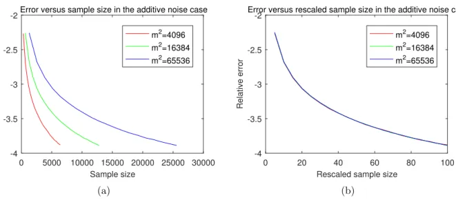
The first experiment is performed to demonstrate the statistical guarantee for multi-response linear regression in additive noise and missing data cases, respectively. Fig. 1(a) plots the relative error on a logarithmic scale versus the sample size n for three different ma-trix dimensionsd∈ {64,128,256}in the additive noise case. For each matrix dimension, as the sample size increases, the relative error decreases to zero, implying the statistical consistency of the estimators. However, larger matrices need larger sample sizes, which is reflected by the rightward shift of the curves as the dimension d is increased. Fig. 1(b) shows the same set of simulation results as in Fig. 1(a), but now the relative error is plotted versus the rescaled sample size n/m. We can see from Fig. 1(b) that the three curves nearly match with one another under different matrix dimensionsd, coinciding with Corollary 1. Hence, Fig. 1 shows that n/d actually acts as the effective sample size in this high-dimensional setting. Similar results on the statistical consistency for the missing data case are displayed in Fig. 2.
0 5000 10000 15000 20000 25000 30000 Sample size -4 -3.5 -3 -2.5 -2 Relative error
Error versus sample size in the additive noise case m2=4096 m2=16384 m2=65536
(a)
0 20 40 60 80 100
Rescaled sample size -4 -3.5 -3 -2.5 -2 Relative error
Error versus rescaled sample size in the additive noise case
m2=4096 m2=16384 m2=65536
(b)
Figure 1: Statistical consistency for multi-response regression with additive error.
0 5000 10000 15000 20000 25000 30000 Sample size -3 -2.5 -2 -1.5 -1 Relative error
Error versus sample size in the missing data case
m2=4096
m2=16384
m2=65536
(a)
0 20 40 60 80 100
Rescaled sample size -3 -2.5 -2 -1.5 -1 Relative error
Error versus rescaled sample size in the missing data case
m2=4096 m2=16384 m2=65536
(b)
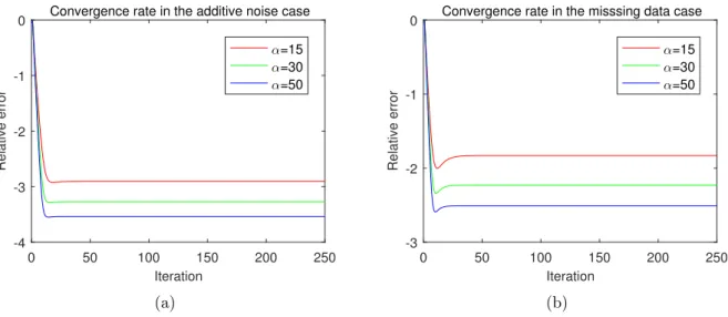
The second experiment is designed to illustrate the algorithmic linear convergence rate in additive noise and missing data cases, respectively. We have investigated the performance for a broad range of dimensionsdandn, and the results are comparatively consistent across these choices. Hence we here report results for p = 128 and a range of the sample sizes n =dαde
with α ∈ {15,30,50}. In the additive noise case, we can see from Fig. 3(a) that for the three sample sizes, the algorithm reveal exact linear convergence rate. As the sample size becomes larger, the convergence speed turns faster and achieves a more accurate estimation level. Fig. 3(b) depicts analogous results to Fig. 3(a) in the case of missing data.
0 50 100 150 200 250 Iteration -4 -3 -2 -1 0 Relative error
Convergence rate in the additive noise case α=15 α=30 α=50 (a) 0 50 100 150 200 250 Iteration -3 -2 -1 0 Relative error
Convergence rate in the misssing data case α=15 α=30 α=50
(b)
Figure 3: Algorithmic convergence rate for multi-response regression with measurement error.
Appendix A
Technical lemmas
In this appendix, several technical lemmas are provided , which are used to establish proposi-tions on RSC/RSM condiproposi-tions and deviation condiproposi-tions for different observation models (cf. Propositions 1–4). The first three lemmas are in preparation for the RSC/RSM conditions, while the next two lemmas are for the deviation conditions. The following lemma tells us that the intersection of the matrix `1-ball with the matrix `2-ball can be bounded by virtue
of a simpler set. For a symbol x ∈ {0,∗, F} and a positive real number r ∈ R+, define
Mx(r) = {A∈Rd1×d2||||A|||x ≤r}, where|||A|||0 denotes the rank of matrix A.
Lemma A.1. For any constant r≥1, it holds that
M∗(
√
r)∩MF(1)⊆2cl{conv{M0(r)∩MF(1)}}, (A.1)
where cl{·} and conv{·} denote the topological closure and convex hull, respectively.
Proof. Note that when r > min{d1, d2}, this containment is trivial, since the right-hand
set is equal to MF(2), and the left-hand set is contained in MF(1). Thus, we will assume
1≤r≤min{d1, d2}.
Let A ∈ M∗(
√
r)∩MF(1). Then it follows that |||A|||∗ ≤
√
r and |||A|||F ≤ 1. Consider a singular value decomposition of A:
where U ∈ Rd1×d1 and V ∈ Rd2×d2 are orthogonal matrices, and D ∈
Rd1×d2 consists of σ1(D), σ2(D),· · · , σk(D) on the “diagonal” and 0 elsewhere with k = rank(A). Write D =
diag(σ1(D), σ2(D),· · · , σk(D)), and use vec(D) to denote the vectorized form of the matrix
D. Then it follows thatkvec(D)k1 ≤
√
r and kvec(D)k2 ≤1. Partition the support of vec(D)
into disjoint subsetsT1, T2,· · ·, such thatT1 is the index set corresponding to the firstrlargest
elements in absolute value of vec(D),T2 indexes the nextr largest elements, and so on. Write
Di = diag(vec(D)Ti), and Ai = U DiV
>
. Then one has that |||Ai|||0 = rank(Ai) ≤ r and
|||Ai|||F ≤ 1. Write Bi = 2Ai/|||Ai|||F and ti = |||Ai|||F/2. Then Bi ∈ 2{M0(r) ∩MF(1)}}
and ti ≥ 0. Now we check that A can be expressed as a convex combination of matrices in
2{conv{M0(r)∩MF(1)}}, namelyA=Pi≥1tiBi. Since the zero matrix contains in 2{M0(r)∩
MF(1)}, it suffices to show that
P
iti ≤ 1, which is equivalent to
P
i≥1kvec(D)Tik2 ≤ 2. To prove this, first note that kvec(D)T1k2 ≤ kvec(D)k2. Second, note that for i ≥ 2, each
elements of vec(D)Ti is bounded in magnitude by kvec(D)Ti−1k1/r, and thus kvec(D)Tik2 ≤
kvec(D)Ti−1k1/
√
r. Combining these two facts, one has that
X i≥1 kvec(D)Tik2 ≤1 + X i≥2 kvec(D)Tik2 ≤1 + X i≥2 kvec(D)Ti−1k1/ √ r≤1 +kvec(D)k1/ √ r≤2.
The proof is complete.
For ease of notation, define the sparse setK(r) :=M0(r)∩MF(1) and the cone setC(r) := {A∈Rd1×d2
|||A|||∗ ≤
√
r|||A|||F}.
Lemma A.2. Let Γ∈Rd1×d1 be a fixed matrix, r ≥1, and δ >0 be a tolerance. Suppose that
the following condition holds
|hhΓ∆,∆ii| ≤δ, ∀∆∈K(2r). (A.3) Then we have that
|hhΓ∆,∆ii| ≤12δ(|||∆|||2F +1
r|||∆|||
2
∗), ∀∆∈R
d1×d2. (A.4)
Proof. We begin by establishing the inequalities
|hhΓ∆,∆ii| ≤12δ|||∆|||F2, ∀∆∈C(r), (A.5a)
|hhΓ∆,∆ii| ≤ 12δ r |||∆|||
2
∗, ∀∆∈/ C(r), (A.5b)
then (A.4) then follows directly.
Now we turn to prove (A.5). By rescaling, (A.5a) holds if we can show that
|hhΓ∆,∆ii| ≤12δ, for all ∆ satisfying |||∆|||2F = 1 and|||∆|||∗ ≤√r. (A.6) It then follows from Lemma A.1 and continuity that (A.6) can be reduced to the problem of proving that
|hhΓ∆,∆ii| ≤12δ, ∀∆∈2conv{K(r)}= conv{M0(r)∩MF(2)}. (A.7)
For this purpose, consider a weighted linear combination of the form ∆ = P
iti∆i, with
weights ti ≥0 such that Piti = 1, and |||∆i|||0 ≤r and |||∆i|||F ≤2 for each i. Then one has
that hhΓ∆,∆ii=hhΓ(X i ti∆i),( X i ti∆i)ii= X i,j titjhhΓ∆i,∆jii.