A Constrained Multi-Objective Learning Algorithm for Feed-Forward Neural Network Classifiers

A Constrained Multi-Objective Learning Algorithm

for Feed-Forward Neural Network Classifiers

Mohamed Njah

Control and Energy Management laboratory (CEM Lab) Digital Research Center of Sfax, Tunisia

[email protected]

Ridha El Hamdi

Control and Energy Management laboratory (CEM Lab) Digital Research Center of Sfax, Tunisia

[email protected]

Abstract—This paper proposes a new approach to address the optimal design of a Feed-forward Neural Network (FNN) based classifier. The originality of the proposed methodology, called CMOA, lie in the use of a new constraint handling technique based on a self-adaptive penalty procedure in order to direct the entire search effort towards finding only Pareto optimal solutions that are acceptable. Neurons and connections of the FNN Classifier are dynamically built during the learning process. The approach includes differential evolution to create new individuals and then keeps only the non-dominated ones as the basis for the next generation. The designed FNN Classifier is applied to six binary classification benchmark problems, obtained from the UCI repository, and results indicated the advantages of the proposed approach over other existing multi-objective evolutionary neural networks classifiers reported recently in the literature.

Keywords-FNN Classifier; Constrained Multi-Objective Optimization; Pareto Dominance Criterion; Differential Evolution

I. INTRODUCTION

The problem of classification is perhaps one of the most widely studied in the data mining and machine learning communities. Classification tasks are widely used in real-world applications, including handwritten characters, detection of faces in images, medical diagnosis and several other tasks [1]. Moreover, there are a large number of computational classification systems that are commonly used for classification, such as probabilistic methods, decision trees, rule-based methods, instance-based methods, SVM techniques, and neural networks [2, 3]. All these modeling techniques tackle the problem of dividing between two or more classes. Classification problems involving multiple classes can be addressed in different ways. One of the most popular techniques consists in dividing the original dataset into two-class subsets, learning a different binary model for each new subset. This work focuses on Feed-forward Neural Network (FNN) based classifiers for solving two-class classification tasks, that is, classifiers that assign patterns to one of two different classes, typically denoted as positive and negative classes. FNN based classifiers [4] have attracted a lot of research effort during the last 20 years, and they are still one of

the hottest research topics in the field of machine learning because of their learning and generalization capability. This however does not imply that a FNN can easily learn the underlying functional mapping between the input data and the desired output. In fact, the main drawbacks of FNNs are problems associated with local minima and the slow convergence of the learning process. Population-based stochastic search approaches, such as evolutionary algorithms (EA), have been proposed to address the problem of the optimal design of the whole (i.e., input vector, structure, and weights) FNN, since such methods are particularly useful for dealing with complex problems having large search spaces with many local optima. A comprehensive review of these approaches can be found in [5]. However, the use of EA in FNN does not emphasize the trade-off between complexity and accuracy of the FNN based classifier. This trade-off is a well-known problem in the multi-objective optimization field.

In recent years, Pareto-based multi-objective algorithms [6] have been adopted for the design of FNN and they have attracted much interest, with promising results. Such approaches are usually implemented by means of error minimization while controlling the complexity of the model [6]. In addition, it is generally known, in the framework of binary classifiers, that the sensitivity and the specificity which express, respectively, how well the system classifies patterns belonging to the positive class and to the negative class are also conflicting objectives [7]. Therefore, to deal with this antagonism, the use of multi-objective optimization within the evolutionary neural network classifier seems an expected headway.

This paper proposes a new Constrained Multi-Objective Optimization Algorithm (CMOA) to achieve a solution to the learning of a FNN based classifier, characterized by good generalization properties. Hence, the primary goal in CMOA is to find or to approximate the set of Pareto optimal solutions [8] that results into trade-offs among learning performance (expressed in terms of sensitivity and specificity) and complexity. However, this Pareto front includes unacceptable solutions. Indeed, it is well known that for each application we could, beforehand, attribute a threshold on the learning

F_m=2*Recall*Precision Recall+Precision Precision= TP TP+FP and Recall= TP TP+FN     1 1 m (2) f min F

performance of the desired neural network. If the learning performance is greater than some value, the associated classifier is then considered as unacceptable solution. Therefore, CMOA aim at splitting objective space into two areas separating the acceptable solutions from unacceptable ones and uses a specific constraint handling technique based on a self-adaptive penalty procedure in order to direct the entire search effort towards finding only Pareto optimal solutions that are acceptable.

II. RELATED WORKS

Several approaches have been proposed to address the problem of the optimal design of neural network based classifier such as constructive [9], pruning [10], regularization [11] and population-based stochastic search approaches [4]. These approaches, usually, jointly minimize network complexity and empirical error in the form of a single loss-function that usually consists of an error cost loss-function and a regularizer. Although this may result in good generalization models, they are highly dependent on user defined training parameters. In addition, it is generally known that error and complexity are conflicting objectives [6], e.g. reducing the approximation error often leads to an increase of the complexity of the model and consequently, no single optimal solution exists that optimizes all the objectives simultaneously. This viewpoint led to the development of multi-objective machine learning (MOML) methods [6].

In recent years, several studies discussed the use of multi-objective approaches, as more promising algorithms, for automatic design of NN-Classifiers. In [12], authors proposed a Multi-Objective Evolutionary Algorithm called PDE (Pareto Differential Evolution), for vector optimization problems. PDE algorithm includes differential evolution to create new individuals and then keeps only the non-dominated ones as the basis for the next generation. From the onset of the PDE algorithm, and almost in parallel, Memetic (i.e. evolutionary algorithms (EAs) augmented with local search) Pareto artificial neural network (MPANN), which is a version of PDE with a local search algorithm, was developed in [13] to optimize the number of hidden nodes and the training of ANNs. In [14], an MPANN is applied to breast cancer diagnosis and promising results have been obtained. In [15], PDE is used to generate a Pareto optimal set of artificial neural networks that act as controllers for the legged locomotion of a quadrupedal robot simulated in a 3-dimensional, physics-based environment.

Other studies have focused on the problem of multi-objective optimization of NN-Classifiers as powerful tools in the domain of face detection [16]. According to [17], the developed hybrid evolutionary algorithm using either scalar fitness or the NSGA-II selection scheme [18] successfully solves the problem of reducing the number of hidden neurons of the NN-Classifier without loosing detection accuracy. More recently, in [6] authors provided an overview of the existing research on Pareto-based multi-objective learning algorithms. A number of machine learning case studies are provided to show the main benefits of the Pareto-based approach versus Single-Objective Learning. Three approaches of Pareto-based multi-objective ensemble generation are compared and discussed, in terms of how to generate classifiers, how to

choose which classifier among them and which ones have formed the ensemble. Pareto-based multi-objective algorithms have been also adopted for the design of Radial Basis Function Networks (RBFNs) and they have attracted much interest in recent years, with promising results [19-21]. In [22], authors studied the use of specific techniques for selecting the best artificial neural model with sigmoid basis units from a Multi-Objective Evolutionary Algorithm called MPDENN algorithm based on the PDE algorithm [12] and on the local search algorithm iRprop [23]. These techniques are based on choosing the best models for training in the two objectives, the correct classification rate and the minimum sensitivity. These techniques are compared with three standard selection methodologies with very promising results.

III. BACKGROUND MATERIALS

A. Performance Measures

In the framework of FNN based classifiers, the accuracy of a classifier is, usually, evaluated in terms of percentage of correct classifications, and the objective of a classifier identification process is to maximize this percentage. This objective might not be appropriate for the application domains characterized by highly imbalanced distributions of patterns, with positive cases composing just a small fraction of the available data used to train the classifier, or when the cost of misclassification of the positive patterns is different from the cost of misclassification of the negative patterns [24]. In order to avoid these deficiencies, other evaluation measures [25] have been defined in the literature. Generally, these evaluation metrics are built from a confusion matrix (Table I).

TABLE I. CONFUSION MATRIX FOR A TWO-CLASS CLASSIFICATION TASK

Decision: Prediction Class

Positive Negative

True Class

Positive True Positives (TP) False Negatives (FN)

Negative False Positives (FP) True Negatives (TN)

Based on the confusion matrix, a popular measure has been proposed [7] as one of the most relevant metric to imbalanced data. This measure, called F-measure (Fm), is defined as the

harmonic mean of recall and precision:

(1)

where

The recall, also known as sensitivity or true positive rate, refers to the proportion of samples belonging to the positive class (true positives), which were correctly predicted as positive. Precision is the proportion of true positive samples among all samples that are predicted as being positive.

B. Pareto Fitness Assignment

The two objectives that are considered, under the CMOA approach, to control the learning performance and the complexity of the FNN based classifier are:

S_i=ni N

η=1−R_a

R_a=Nb of acceptable solutions_{population size}

3 1 2 0 ( ( )) 0.5 (8) 1 p p p c i i i i if Y F Y Y Y = íìïï + - £ ïïî 3 1 2 1 ( ) [0 (7) ,1] p p p c i i i i p i X F X X if U CR X X else ìï + - £ ï = í ïïî

{

}

The minimization of the L2_norm of hidden-layer weights

(f2) is a conventional manner to control the size of the network

complexity [26]. In our problem formulation, we use only one hidden layer of neurons, as dictated by the universal approximation capability theorem for neural networks [27].

The CMOA approach includes differential evolution [28] to create new individuals and then keeps only the non-dominated ones as the basis for the next generation. The population is sorted according to the Pareto dominance concept [6]. Once a Pareto front is built, each individual i in the Pareto front (a non-dominated solution) is assigned a fitness value Fi.

(4 1 ( 1) ) i i i S if i is an acceptable solution F S h otherwise ì + ïï = í_{ï +} ïî The fitness value of an individual i depends on its strength value Si[0, 1], representing the number of solutions it

dominates, divided by the population size N.

(5)

If the individual is unacceptable, a penalty factor [0, 1] is used.

(6)

where

In (4), 1 is added to ensure that the fitness value of an individual is greater than zero. This is quite interesting because not only individuals that correspond to the two extremes of the Pareto front may have null strength values (they are not dominated by any of the individuals of the population) but also individuals that correspond to the middle of the Pareto front, especially in last generations. Moreover, the use of a self-adaptive penalty (SAP) procedure based on the penalty factor  is very promising since it requires no parameter tuning. The method keeps track of the percentage of acceptable individuals in the population (as illustrated in Figure 1) to determine the amount of penalty applied to unacceptable individuals. If there are a few acceptable individuals in the whole population (usually in early generations), a penalty factor (1Σφάλμα! Τα

αντικείμενα δεν μπορούν να δημιουργηθούν από την επεξεργασία κωδικών πεδίων.) is applied to unacceptable solutions. Otherwise, a penalty factor (0) is used. As discussed earlier, CMOA aims at splitting objective space into two areas, separating the acceptable solutions from unacceptable ones and uses a constraint handling technique based on a self-adaptive penalty method so as to direct the entire search effort towards finding only Pareto optimal solutions that are acceptable.

C. Differential Evolution

Differential evolution (DE) [28] is a simple, but powerful algorithm that simulates natural evolution combined with a mechanism of generation of multiple search directions based

on the distribution of solutions (vectors) in the current population. In DE, a child is generated applying the crossover operator to three parents (p1, p2 and p3). The resultant child is a

perturbation of the main parent (p1).

a- Only 12 percent of solutions are acceptable

b- 68 percent of solutions are acceptable

Fig. 1. Illustration of fitness computation for CMOA with regard to the percentage of acceptable solutions

If we consider Xip1, Xip2 and Xip3 the ith parametric genes

respectively of parents p1, p2 and p3, the ith parametric gene of

the child C (i.e. Xic) is generated as follows:

Where F[0, 1] is an amplification factor also called "differential weight". CR is the rate of crossover and U is a random fraction in the [0, 1] interval.

Once the child parametric genes are generated, we proceed to apply the same principle of differential evolution for structural genes to determine the structure of the child to generate.

If we consider Yip1, Yip2 and Yip3 the ith structural genes

respectively of parents p1, p2 and p3, the ith structural gene of

Yes

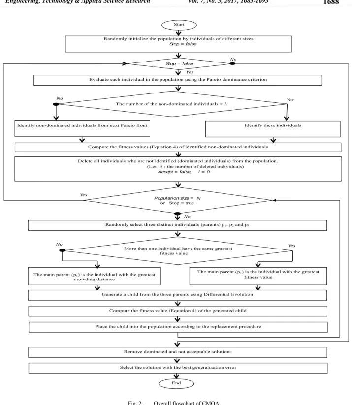
Randomly initialize the population by individuals of different sizes Stop = false

Evaluate each individual in the population using the Pareto dominance criterion

Identify non-dominated individuals from next Pareto front

The number of the non-dominated individuals > 3

Identify these individuals

Compute the fitness values (Equation 4) of identified non-dominated individuals Delete all individuals who are not identified (dominated individuals) from the population.

(Let E : the number of deleted individuals) Accept = fal se, i = 0

Popul ation size = N or Stop = true

Randomly select three distinct individuals (parents) p1, p2 and p3

No

No _Yes

Yes

No

The main parent (p1) is the individual with the greatest

crowding distance

More than one individual have the same greatest fitness value

The main parent (p1) is the individual with the greatest

fitness value

No _Yes

Generate a child from the three parents using Differential Evolution

Compute the fitness value (Equation 4) of the generated child

Place the child into the population according to the replacement procedure

Remove dominated and not acceptable solutions Stop = false

Select the solution with the best generalization error

End Start

Fig. 2. Overall flowchart of CMOA

IV. CONSTRAINED MULTI-OBJECTIVE OPTIMIZATION ALGORITHM (CMOA)

The proposed CMOA approach can be described as shown in Figure 2. The algorithm starts generating a random population of individuals of different sizes. The population is sorted according to the non-domination concept and dominated individuals are removed from the population. The remaining non-dominated solutions are retained for reproduction. As the

DE strategy requires at least three different non-dominated individuals, we allow the algorithm to consider the non-dominated individuals of the second Pareto front if the first edge is composed of only one or two individuals. Three parents are selected at random. The individual with the best fitness value (4) is considered as the main parent and the other two as supporting parents. If more than one parents share the same best fitness value, a crowding distance measure [18] was used

to select the main parent in order to produce and maintain well-distributed solutions.

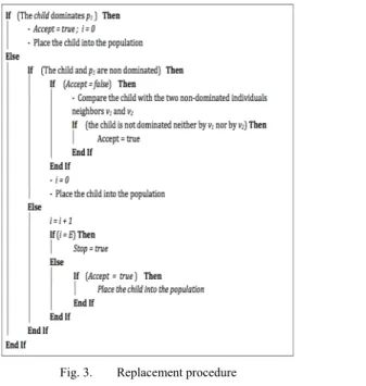
A child is generated from the three parents and is placed into the population according to a replacement procedure (Figure 3). This process continues until the population is completed.The replacement procedure is used so as to ensure convergence of the algorithm. In fact, it attempts, from one generation to another:

 To improve the quality of the Pareto frontier by adding at least one offspring individual that dominates his main parent.

 Or to increase the number of Pareto optimal solutions on the Pareto frontier by adding at least one offspring individual that is non-dominated with respect to the current sub-population of parents. In other words, the generated child should not, therefore, be dominated neither by v1 nor by v2, where v1 and v2 are the two non-dominated individuals neighbours with regard to the generated offspring.

Iterations are terminated when none of the E generated offspring individuals satisfy the condition of the replacement procedure (E is the same number of deleted individuals in the current population). For the application of the proposed method, we have to select only one preferred solution. To facilitate the selection task, dominated and unacceptable solutions are removed at the end of the multi-objective optimization. The best representative solution is, then, chosen from the remaining Pareto frontier individuals based on the generalization error computed on a test set.

V. EXPERIMENTAL RESULTS

The CMOA approach was developed and implemented using Xcode version 7.2 under a Mac os x 10.11.2 workstation. To examine the performance of CMOA, we consider six benchmark classification problems, selected from the UCI repository. Table II gives a brief description of the selected datasets.

Fig. 3. Replacement procedure

TABLE II. DESCRIPTION OF THE SELECTED DATASETS Dataset Patterns Attributes % Positive % Negative

Breast cancer 683 9 35 65 Australian card 690 14 44.5 55.5 Ionosphere 351 34 64.1 35.9 German 1000 61 70 30 Pima 768 8 34.9 65.1 Heart 270 13 44.45 55.55

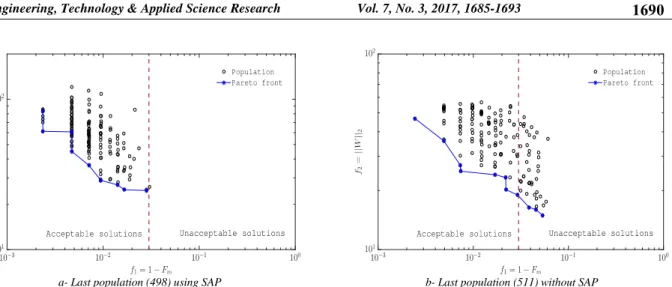
Figure 4 and Figure 5 show the effect of the application of the self-adaptive penalty (SAP) procedure on the final solutions. These results are achieved using respectively the first and the second dataset. These two figures show clearly that the SAP procedure discards unacceptable solutions. Their number becomes very limited at the end of calculations, when the SAP procedure is applied. However, when the SAP procedure is not applied to the algorithm, the proportion of unacceptable solutions remains hight and this influences the quality of the solution obtained at the end of calculation. In terms of computational time, the total number of generations in both cases (using or without SAP) does not seem to differ much. In order to know how competitive the proposed method is, we decided to compare it against two relevant Pareto-based

multi-objective learning algorithms called MPANN and

MPENSGA2.

MPENSGA2 (memetic Pareto evolutionary NSGA2) was introduced in [29]. It tries to boost two conflicting main objectives: the best model in accuracy and the best model in sensitivity. Concretely, a memetic version of NSGA2 [18], which introduces the iRprop+ algorithm [23] as a local optimizer adapted to the softmax activation function and the cross-entropy error function, designs the ANNs architecture finding an adequate number of neurons in the hidden layer and an adequate number of connections along with their corresponding weights. The comparison was conducted using a stratified holdout procedure with 30 runs, where approximately 75% of the patterns were randomly selected for the training set and the remaining 25% for the test set.

In each execution, once the first Pareto front is calculated, we chose the extreme values in training, that is, the best individual in the two objectives that are considered. In this paper, we denote :

 M1: the methodology using the proposed CMOA approach and the extreme chosen individual is the one that has better learning performance (2).

 M2: the methodology using the proposed CMOA approach and the extreme chosen individual is the one that has better complexity of the FNN based classifier (3).

 M3: the methodology using the MPENSGA2 approach and the extreme chosen individual is the one that has better entropy.

 M4: the methodology using the MPENSGA2 approach and the extreme chosen individual is the one that has better sensitivity.

a- Last population (498) using SAP b- Last population (511) without SAP Fig. 4. Effect of the use of the self-adaptive penalty (SAP) procedure on the final solutions (Breast cancer)

a- Last population (490) using SAP b- Last population (500) without SAP Fig. 5. Effect of the use of the self-adaptive penalty procedure on the final solutions (Australian Card)  M5: the methodology using the MPANN approach and the

extreme chosen individual is the one that has better error (MSE).

 M6: the methodology using the MPANN approach and the extreme chosen individual is the one that has better ANN complexity (number of hidden units).

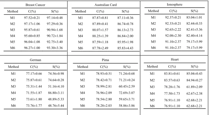
Table III presents the values of average and standard deviation for accuracy and sensitivity for the testing set of each dataset obtained for the best models in each run. Statistical results achieved from MPENSGA2 and MPANN are obtained from [29]. A first analysis of the results, illustrated in table III, shows that the performance of the proposed method is competitive or comparable to both MPANN and MPENSGA2. From a statistical point of view, these comparisons are possible because we use the same partitions of the datasets. In other cases, it is difficult to justify the equity of the comparison procedure. The results reported in Table III show also that the developed method CMOA achieves slightly better standard deviation in most datasets. It is interesting to see the small standard deviation for the test performances, which indicates consistency and stability of the used method.

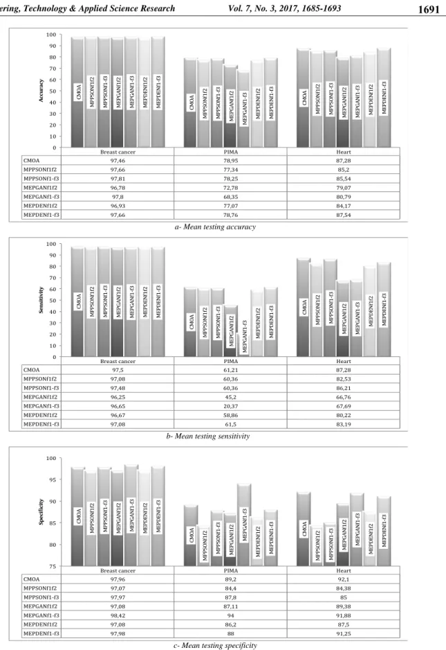
The proposed approach is also compared against three multi-objective learning algorithms, proposed in [19, 20] for the design of Radial Basis Function Networks (RBFNs). These algorithms are named Memetic Pareto Particle Swarm Optimization based RBFN (MPPSON), Memetic Elitist Pareto non-dominated sorting Genetic Algorithm based RBFN (MEPGAN) and Memetic Elitist Pareto non-dominated sorting Differential Evolution based RBFN (MEPDEN). These algorithms have been tested based on two and three objective functions. The first one (f1) is the accuracy based on Mean-Squared Error (MSE) on the training set. The second objective function (f2) concerns the complexity of RBF network and is computed based on the number of hidden nodes in the hidden layer. The last one (f3) concerns also the complexity of the network and is computed based on the norm of the centers and weights of the RBF network. The comparison was carried out on the same datasets used in both this paper and those two references [19, 20], i.e. the first and the last two datasets shown in Table II. The results were obtained by 10-fold cross-validation for all datasets. Each dataset is divided into ten subsets of equal size. One subset is used as the testing dataset, and the other nine subsets are used as the training dataset.

Breast cancer PIMA Heart CMOA 97,46 78,95 87,28 MPPSONf1f2 97,66 77,34 85,2 MPPSONf1-f3 97,81 78,25 85,54 MEPGANf1f2 96,78 72,78 79,07 MEPGANf1-f3 97,8 68,35 80,79 MEPDENf1f2 96,93 77,07 84,17 MEPDENf1-f3 97,66 78,76 87,54 CM OA CM OA _CMO A M PP SO N f1 f2 MP PS O N f1 f2 M PPS O N f1 f2 MP PS O N f1 -f 3 M PPS O N f1 -f 3 M PPS O N f1 -f 3 ME PG A N f1 f2 ME PG A N f1 f2 ME PG A N f1 f2 ME PG A N f1 -f 3 ME PG A N f1 -f 3 ME PG A N f1 -f 3 M EP D EN f1 f2 M EP D EN f1 f2 ME PD EN f1 f2 ME PD EN f1 -f 3 ME PD EN f1 -f 3 ME PD EN f1 -f 3 0 10 20 30 40 50 60 70 80 90 100 Ac cu ra cy

a- Mean testing accuracy

Breast cancer PIMA Heart

CMOA 97,5 61,21 87,28 MPPSONf1f2 97,08 60,36 82,53 MPPSONf1-f3 97,48 60,36 86,21 MEPGANf1f2 96,25 45,2 66,76 MEPGANf1-f3 96,65 20,37 67,69 MEPDENf1f2 96,67 58,86 80,22 MEPDENf1-f3 97,08 61,5 83,19 CM OA CM O A CM O A M PP SO N f1 f2 MP PS O N f1 f2 M PP SO N f1 f2 MP PS O N f1 -f 3 M PPS ON f1 -f 3 M PPS O N f1 -f 3 ME PG A N f1 f2 ME PG A N f1 f2 ME PG A N f1 f2 ME PG A N f1 -f 3 ME PG A N f1 -f 3 ME PG A N f1 -f 3 ME PD EN f1 f2 M EP D EN f1 f2 M EP D EN f1 f2 MEP D EN f1 -f 3 ME PD EN f1 -f 3 ME PD EN f1 -f 3 0 10 20 30 40 50 60 70 80 90 100 Se n sit iv it y

b- Mean testing sensitivity

Breast cancer PIMA Heart

CMOA 97,96 89,2 92,1 MPPSONf1f2 97,07 84,4 84,38 MPPSONf1-f3 97,97 87,8 85 MEPGANf1f2 97,08 87,11 89,38 MEPGANf1-f3 98,42 94 91,88 MEPDENf1f2 97,08 86,2 87,5 MEPDENf1-f3 97,98 88 91,25 CM OA CM O A CM O A M PP SO N f1 f2 M PP SO N f1 f2 M PP SO N f1 f2 MPP SO N f1 -f 3 M PPSON f1 -f 3 M PPS ON f1 -f 3 M EP G A N f1 f2 M EP G A N f1 f2 ME PG A N f1 f2 ME PG A N f1 -f 3 ME PG A N f1 -f 3 ME PG A N f1 -f 3 M EP D EN f1 f2 M EP D EN f1 f2 ME PD EN f1 f2 ME PD EN f1 -f 3 ME PD EN f1 -f 3 ME PD EN f1 -f 3 75 80 85 90 95 100 Speci icity

c- Mean testing specificity

This train and test process is repeated so that all subsets are used as a testing dataset. The summary of performance comparisons of proposed and existing methods on the testing set is shown in Figure 6. It can be observed from Figure 6 that, for the breast cancer dataset, there are no significant differences between the analyzed methods in terms of accuracy and sensitivity. However, in terms of specificity, it can be observed that the proposed CMOA approach outperforms algorithms using two objective functions (MPPSONf1f2, MEPGANf1f2 and MEP DENf1f2) and is competitive to algorithms using three objective functions (MPPSONf1-f3, MEPGANf1-f3 and MEPDENf1-f3). For Pima and Heart datasets, CMOA is better or at least competitive to other algorithms except MEPGANf1f2 which has demonstrated the best specificity values (94 %) for Pima dataset. However, for this dataset,

MEPGANf1f2 performs poorly, in terms of accuracy and sensitivity, with respect to other algorithms.

VI. CONCLUSION

This study constructs a novel methodology for implementing Pareto-based multi-objective optimization within the evolutionary neural network classifier. Using six binary classification benchmark problems, obtained from the UCI repository, the proposed approach was shown to be competitive to older works. The results gave also a useful insight on the impact of using the self-adaptive penalty (SAP) procedure. For future work, we will evaluate the performance of the proposed method on regression problems. Another interesting issue that rises from this work is how to extend the proposed methodology to work with other kind of classifiers.

TABLE III. MEAN TESTING ACCURACY C(%) AND SENSITIVITY S(%) FOR THE DIFFERENT METHODS

Breast Cancer Method C(%) S(%) M1 97.52±0.21 97.14±0.48 M2 97.17±1.06 97.29±0.36 M3 95.87±0.61 90.94±1.68 M4 95.60±0.85 90.72±1.84 M5 96.04±1.08 92.75±3.40 M6 96.27±1.00 93.30±3.36 Australian Card Method C(%) S(%) M1 87.87±0.81 87.11±0.36 M2 87.89±0.41 86.74±0.78 M3 88.07±1.57 86.13±2.73 M4 88.25±1.39 86.84±2.00 M5 87.59±1.18 85.95±1.98 M6 87.78±2.49 85.83±4.43 Ionosphere Method C(%) S(%) M1 92.37±0.21 83.04±1.01 M2 92.33±0.21 82.44±0.33 M3 92.65±2.22 82.41±5.36 M4 92.08±2.30 82.40±4.14 M5 91.10±2.37 79.17±5.99 M6 91.10±2.37 79.17±5.99 German Method C(%) S(%) M1 77.17±0.66 74.56±0.98 M2 75.87±0.61 74.64±0.28 M3 75.31±1.44 51.16±4.10 M4 71.55±1.87 86.80±3.11 M5 73.61±1.80 48.89±5.33 M6 73.76±1.77 48.76±5.44 Pima Method C(%) S(%) M1 78.93±0.51 71.24±0.68 M2 78.42±0.71 71.21±0.24 M3 78.99±2.81 60.45±2.59 M4 76.96±2.09 72.69±3.07 M5 78.54±2.80 59.65±3.71 M6 78.28±2.03 58.86±3.86 Heart Method C(%) S(%) M1 83.81±0.61 85.04±0.43 M2 83.57±0.63 84.94±0.27 M3 78.28±1.76 61.89±2.09 M4 77.50±1.73 62.67±2.38 M5 76.91±1.10 62.68±2.21 M6 76.91±1.10 62.68±2.21 REFERENCES

[1] C. Aggarwal, Data Classification: Algorithms and Applications, 1st Edition. Chapman and Hall/CRC, 2014

[2] R. Ramli, H. Arof, F. Ibrahim, M. Y. I. Idris, A. S. M. Khairuddin, “Classification of Eyelid Position and Eyeball Movement Using EEG Signals”, Malaysian Journal of Computer Science. Vol. 28, No. 1, pp. pp. 28-45, 2015

[3] S. M. A. Kalaiarasi, S. Gopala, C. Ali, T. Jason, “Artificial Neural Network Tree Approach In Data Mining”, Malaysian Journal of Computer Science, Vol. 20, No. 1, pp. 51-62, 2007

[4] V. Chaitali, B. Nikita, M. Darshana, “A survey on various classification techniques for clinical decision support system” International Journal of Computer Applications, Vol. 116, No. 23, pp. 14–17, 2015

[5] A. Azzini, A. G. B. Tettamanzi, “Evolutionary ANNS: a state of the art survey”, Intelligenza Artificiale,Vol. 5, pp. 19–35, 2011

[6] Y. Jin, B. Sendhoff, “Pareto-based multi-objective machine learning: An overview and case studies”, IEEE Transactions on Systems, Man, and

Cybernetics Part C: Applications and Reviews, Vol. 38, No. 3, pp. 397– 415, 2008

[7] T. Fawcett, “An introduction to roc analysis”, Pattern Recognition Letters, Vol. 27, No. 3, pp. 861–874, 2006

[8] J. Fieldsend, S. Singh, “Pareto evolutionary neural networks”, IEEE Transactions on Neural Networks, Vol. 16, No. 2, pp. 338–354, 2005 [9] S. K. Sharma, P. Chandra, “Constructive neural networks: A review”,

International Journal of Engineering Science and Technology, Vol. 2, No. 12, pp. 7847–7855, 2010

[10] A. Engelbrecht, “A new pruning heuristic based on variance analysis of sensitivity information”, IEEE Transactions on Neural Networks, Vol. 11, No. 6, pp. 1386–1399, 2011

[11] H. Chen, Diversity and Regularization in Neural Network Ensembles, Ph.D. Thesis, School of Computer Science University of Birmingham, 2008

[12] H. A. Abbass, R. Sarker, C. Newton, “PDE: a pareto-frontier differential evolution approach for multi-objective optimization problems”, 2001 Congress on Evolutionary Computation, Seoul, South Korea, pp. 971– 978, 2001

[13] H. A. Abbass, “A memetic Pareto evolutionary approach to artificial neural networks”, Australian Joint Conference on Artificial Intelligence, pp. 1–12, 2001

[14] H. A. Abbass, “An evolutionary artificial neural network approach for breast cancer diagnosis”, Artificial Intelligence in Medicine, Vol. 25, pp. 265–281, 2002

[15] J. Teo, “Evolutionary Multi-Objective Optimization For Automatic Synthesis Of Artificial Neural Network Robot Controllers”, Malaysian Journal of Computer Science, Vol. 18, No. 2, pp. 54-62, 2005.

[16] K. Krawiec, W. Jaskowski, M. Szubert, “Multi-objective convolutional learning for face labeling”, IEEE Conference on Computer Vision and Pattern Recognition (CVPR), pp. 3451-3459, 2015

[17] S. Wiegand, C. Igel, “Evolutionary multi-objective optimization of neural networks for face detection”, International Journal of Computational Intelligence and Applications, Vol. 4, No. 3, pp. 237– 253), 2004

[18] K. Deb, A. Pratab, S. Agarwal, T. Meyarivan, “A fast and elitist multi-objective genetic algorithm: NSGA2”, IEEE Transactions on Evolutionary Computation, Vol. 6, No. 2, pp. 182–197, 2002

[19] N. Q. Sultan, M. S. Siti, M. Z. Azlan, “Multi-objective hybrid evolutionary algorithms for radial basis function neural network design”, Knowledge-Based Systems. Vol. 27, pp. 475–497, 2012

[20] N. Q. Sultan, M. S. Siti, Z. M. H. Siti, “Memetic multiobjective particle swarm optimization based radial basis function network for classification problems”, Information Sciences, Vol. 239, pp. 165–190, 2013

[21] I. Kokshenev, A. Padua Braga, “An efficient multi-objective learning algorithm for RBF neural network”, Neurocomputing, Vol. 73, pp. 2799–2808, 2010

[22] M. Cruz-Ramirez, J. C. Fernandez, J. Sanchez-Monedero, C. Hervas-Martinez, “Memetic Pareto differential evolutionary artificial neural networks to determine growth multi-classes in predictive microbiology”, Evolutionary Intelligence, Vol. 3, pp. 187–199, 2010

[23] C. Igel, M. Husken, “Improving the Rprop learning algorithm”, Second International ICSC Symposium on Neural Computation (NC 2000, pp. 115–121, 2000

[24] P. Ducange, B. Lazzerini, F. Marcelloni, “Multi-objective genetic fuzzy classifiers for imbalanced and cost-sensitive datasets”, Soft Computing, Vol. 14, pp. 713–728, 2010

[25] C. Ferri, J. Hernndez-Orallo, R. Modroiu, “An experimental comparison of performance measures for classification”, Pattern Recognition Letters, Vol. 30, pp. 27–38, 2009

[26] P. L. Bartlett, “The sample complexity of pattern classification with neural networks: The size of the weights is more important than the size of the network”, IEEE Transactions on Information Theory, Vol. 44, No. 2, pp. 525–536, 1998

[27] G. Dreyfus, J. Martinez, M. Samuelides, M. B. Cordon, F. Badran, S. Thiria, L. Herault, Réseaux de neurones: méthodologie et application, Eyrolles, 2004

[28] R. Storn, “Differential evolution research-Trends and open questions”, Studies in Computational Intelligence, Vol. 143, pp. 1-31, 2008 [29] J. C. Fernandez Caballero, F. C. H. José Martinez, P. A. Gutiérrez,

“Sensitivity versus accuracy in multiclass problems using memetic Pareto evolutionary neural networks”, IEEE Transactions on Neural Networks, Vol. 21, No. 5, pp. 750–770, 2010